
New Retailing Problem for an Integrated Food Supply Chain in the Baking Industry


1
Department of Business Administration, Chaoyang University of Technology, Taichung 41349, Taiwan
2
School of Economics and Management, Huizhou University, Huizhou 516007, China
3
Department of Marketing and Logistics Management, Chaoyang University of Technology, Taichung 41349, Taiwan
4
Faculty of Economics, Tay Nguyen University, Buon Ma Thuot 630000, Vietnam
*
Author to whom correspondence should be addressed.
Appl. Sci. 2021, 11(3), 946; https://doi.org/10.3390/app11030946
Submission received: 7 December 2020
/
Revised: 14 January 2021
/
Accepted: 18 January 2021
/
Published: 21 January 2021
(This article belongs to the Special Issue Advances in Food Processing (Food Preservation, Food Safety, Quality and Manufacturing Processes))
Abstract
:As coronavirus disease 2019 (COVID-19) continues to spread, online consumption habits in China have changed significantly. Thus, the booming online-to-offline (O2O) food ordering and delivery industry via the online bakery have been changing customers’ food shopping behavior. This article proposes a comparison relying on advanced O2O strategy for a single-vendor-single-retailer integrated system. Three coordination mechanisms consist of revenue-sharing, buy-back, and quantity flexibility contracts have been employed for optimizing the order quantity. Replenishment strategies and temperature for the supply chain members are considered based on the new retailing framework. Herein, the authors suggest an algorithm for the computation of the optimal solution. Lastly, numerical examples and sensitivity analysis are also conducted to clarify the usefulness of the proposed model in the food supply chain. Sensitivity analysis revealed a number of managerial insights. For example, the results obtained under O2O operations can be compared with those obtained under online/offline operations (under various parameters settings) to determine an opportune moment for three coordination mechanisms.
1. Introduction
Several recent studies have appeared to tackle the new retailing (NR) issue, which is the phrase coined by Jack Ma, Alibaba Executive Chairman [1]. Alibaba was significantly implementing NR and online, offline, logistics, and data across the individual value chain to be involved. New retailing is one sector undergoing an Internet of Things (IoT)-driven revolution, as traditional offline retail stores such as convenience stores and supermarkets have become the point of convergence for online and online integration. According to a research report [2], on “China’s Online Shopping Market Research Report” published in 2012 by CNNIC, internet shopping market accounted for about RMB1.26 trillion trading volume. The online-to-offline (O2O) business model will revolutionize the customer experience in retailing, allowing companies to introduce innovative customer services. The study is still at an early stage in evaluating NR, not to mention a paucity of literature on this subject. Du and Jiang [3] evaluated that the offline service quality problems of O2O model in China. E-commerce’s development in the food supply chain has played an essential role in supporting small and medium enterprises (SMEs) to deal with challenges, stimulating domestic demand for bakery, and creating jobs; thus, the term NR is considered as a new concept based on the development of O2O model. Regarding the history line of the O2O term development, which witnessed the booming of the O2O food market in China in recent years, as recommended by Maimaiti et al. [4], more than twenty percent out of China’s total population has already become the customers of the O2O food delivery market. The O2O model’s impact on the optimal power structure of a retail service supply chain was studied by Chen et al. [5]. On the other hand, He et al. [6] identified the role of the competitive O2O model to adapt to multi-store service firms. In the early 20th century, Smith and Sparks [7] stressed that product quality is the most vital factor in the food supply chain. Van der Vorst et al. [8] explained that organizations can gain a competitive edge by incorporating food quality into food supply chain. In understanding quality assurance with food security, Trienekens and Zuurbier [9] presented the process of production and distribution is the major interest under food supply chain. Product quality, costs, and sustainability have been highlighted as important factors that influence the food supply chain model was dealt with by Zanoni and Zavanella [10]. In line with that, numerous studies have also investigated those issues in terms of the food supply chain [11,12,13]. Due to globalization, the complexity of food supply chains is increasingly becoming more complex. The concept of food supply chain traceability has become not just a way to help food manufacturers and retailers ensure food security (ex: temperature controlled), but also creating a linkage among business floors each other. Furthermore, the adoption of the IoT technology into food supply chain management (SCM) to assist with the information management process has gradually become more popular [14,15,16,17]. Early theorization of a single-vendor single-retailer integrated inventory model can be traced back to Goyal [18]. Moreover, to struggle with the rapidly changing market conditions, the supply chain system must have smooth coordination, which is considered the vital key to attaining the flexibility necessary as well as to meet superior logistics processes. Besides, several prior studies also stressed that a sounder theoretical basis for vendor-retailer integrated inventory model [19,20,21,22]. Consequently, these articles have been published that focus on a wide range of the coordination of the supply chain. Unfortunately, there is no existing article published comparing different food supply chain contracts under the new retailing framework. The channel coordination is considering as the critical key parameter of the SCM, which has been obtained by employ the contract to address related problems. The contract is a major concern in a wide variety of applications; examples of contract are wholesale price, revenue sharing, buy-back, or quantity flexibility.
1.1. Revenue-Sharing Contract
The contracting mechanism has been adopted by supply chain members and well-known as a popular method to mitigate risks. Based on the revenue-sharing approach, which has been widely employed in the e-commerce and the manufacturing sector [23,24,25,26,27,28], Govindan and Malomfalean [29] have employed the Stackelberg game theory to propose the framework for comparing those coordination mechanisms.
1.2. Buy-Back Contract
1.3. Quantity-Flexibility Contract
The current market is witnessing fierce competition among the firms to obtain acceptance from consumers. Companies are making an effort to offer new goods for sale while customers struggle with so many brands for their needs. One of the roles of the new products coordinator is to track the status of all products submittals. Manufacturers expected retailers to set valuable orders for them, such as early time or large quantities due to the fact that they must spend a long time for production preparation. Quantity-flexibility contracts are efficient coordination schemes to balance the risk of each side, especially in the manufacturing sector [38,39,40,41,42,43,44] and retailing sector [45]. Three kinds of contracts have been more widely available and conducted in various supply chains. Based on existing literature, the authors illustrated a taxonomy that reflects accepted categories (as represented in Table 1). On the whole, there has been relatively little progress in comparing the three coordination mechanisms until recently.
Table 1 demonstrated the comparison among existing relevant studies under different supply chain. It is hoped that this brief and necessarily oversimplified review will lead to a better understanding of three contracts in supply chain, in order to address these areas of concern by shedding light on the nature of the problems and to maximize profits of each member of a food chain made up of one manufacturer and one retailer with three contracts. Hence, the contribution of this article was to investigate the decision-making of the temperature, order quantity, number of shipments in food supply chain between manufacturer and retailer. It is important to recognize the efforts of three coordination mechanisms, but we lack empirical support.
1.4. Food Security
Temperature control is a major concern in a wide variety of applications such as preserving food (or food security), distribution food, and storage food. It is evident that a key element within these chains is temperature, also in its different forms, as it is a necessary source to guarantee quality-based processes. Shock freezing is widely used in the food industry. However, it is not popular with catering companies that produce their own bread and bakery products. Many companies prefer to use ready-made frozen semi-finished products, rather than to bake them on their own. Center kitchen (CK), also known as the distribution center, is set up as a modern food production base, equipped with complete environmental protection equipment and food processing equipment. From ordering raw materials, food production, to selling food, the center kitchen carries out unified management. CK is a new trend in the food industry where centralized preparation and processing of fresh foods occurs in the catering chains. It is the basic function of CK to process raw food materials purchased in bulk into semi-products and/or products under the dictation of unified requirement on product qualities. However, the proper control and management of temperature is crucial in delivering perishables to consumers and ensuring that those perishables are in good condition and safe to eat. Aung and Chang [46] addressed the approach used to obtain the optimal temperature for multi-commodity refrigerated storage. Lorite et al. [47] developed a critical temperature indicator (CTI) to monitor the supply chain and storage conditions of perishable food products. Kuo and Chen [48] developed an advanced multi-temperature joint distribution for continuously temperature-controlled logistics. For the food manufacturer, positive food security will protect the company’s brand and goodwill. However, “loss of goodwill” has been touched upon in management science textbooks of various business school curricula. Today it is widely accepted that a goodwill cost may be difficult to estimate. Lawrence and Pasternack [49] argued that many businesses do not have any idea what the long-term goodwill cost of an unsatisfied customer might be. Aksen [50] examined the role of loss of customer goodwill on the incapacitated lot-sizing problem over a finite planning horizon. Finn et al. [51] investigated whether the cost of food contamination can result in indirect losses such as lost reputation and goodwill. Mitreva and Gjurevska [52] applied the TQM tool to a bread and baking company in the quality system.
2. Problem Description
New business models have been relentlessly launched in the market due to the rapid advancement of technology and social changes. While internet shopping becomes more efficient and effective, traditional retailers need new digital innovation. An outbreak of coronavirus infection in Wuhan, China, has led to a global epidemic declared a Public Health Emergency of International Concern by the World Health Organization (WHO). COVID-19 is resistant to environment factors, has high penetration ability, and may be lethal. The food supply chain has needed to adjust rapidly to demand-sides shocks, including cake buying and changes in food purchasing patterns as well as planning for any supply-side disruptions due to potential labor shortages and disruptions to transportation and supply networks. However, few empirical studies have been done on this issue. Hobbs [53] proposed an assessment of implication of the COVID-19 pandemic for the food supply chain regarding the growth of the online grocery delivery sector and the extent to which consumers will prioritize “local” food supply chains. Singh et al. [54] investigated an economic model in helping to simulate a responsive food supply chain to match the varying demand and provided decision-making support for rerouting the vehicles during the COVID-19 pandemic. Rizou et al. [55] provided an excellent review of the possible transmission ways of COVID-19 through the food supply chain and environment before developing COVID-19 diagnostic tests. Therefore, we develop an integrated food supply chain system as well as discussing the optimal decisions found to maximize the total profit based on the new retailing framework through COVID-19 pandemic. Transportation issues caused another concern about food quality that concerned products’ temperature control in customers or distribution centers from COVID hot spots. On the other hand, the traditional retailers recognize that COVID-19 will have a significant impact on their business. Online technology can support customer service staff, engage offline-to-online ordering, and gives sales assistants more opportunities to help customers explore their options. As fresh food deteriorates easily, there has been increasing consumer demand for logistics that ensure the timeliness of deliveries. He et al. [56] proposed an agent-based O2O food ordering model (AOFOM) that consists of customers, restaurants, and the online food ordering platform. Wang et al. [57] made a comparison of food shopping with four e-commerce modes: Business-to-consumer (B2C), online-to-offline delivery (O2O Delivery), online-to-offline in store (O2O In-store), and New Retail. Li et al. [58] provided an excellent review of online food delivery platforms. A fairly large body of literature exists on the supply chain. However, within that literature, there is a surprising lack of information on O2O model. Online food delivery provided a critical lifeline during 2020 COVID-19 pandemic for the tens of millions of people quarantined at home. Such research is still in its infancy, but it may have a contribution to make to comparison the understanding of the above three contracts. Next, the empirical evidence is provided in support of the claim. In order to face the highly competitive environment, the following issues were posed by the manufacturer/retailer:
RQ1.
What is the optimal shipment size from manufacturer to the retailer?
RQ2.
What is the optimal temperature in the food supply chain?
RQ3.
What is the optimal order quantity for the retailer?
RQ4.
Which of three coordinated agreements attains the best outcome under new retailing framework?
The main aim of the present article is to use the inventory model to discuss its properties in comparisons with the overall effects of three coordination mechanisms: Revenue sharing, buy-back, or quantity flexibility. The supply chain coordination proposed by Govindan and Malomfalean [29] was used the basis for replicating consumer behavior under O2O environment described above. We addressed the basic two-echelon supply chain proposed by Yang et al. [59]. They investigated single-supplier and single-retailer production and inventory models in both non-cooperative and cooperative situations. Thus, the contribution of this article is in understanding of three coordination mechanisms in the food supply chain. In actuality, however, coordination mechanism is a common problem in supply chain. Little is known about the comparison of the three coordination mechanism in the literature, with most research concentrating on single/two contracts. Moreover, the author suggests that manufacturers should focus on the effect of three coordination mechanisms in the food supply chain. Notations and assumptions will be demonstrated in Section 3, followed by Section 4, which presents the model formulation. Section 5 and Section 6 will show the suggestion in terms of solutions and application example, respectively. Next, in Section 7, a numerical example will be presented as proof for the findings of Section 5 and Section 6 as mentioned. Finally, conclusions are provided in Section 8.
3. Notations and Assumptions
In addition, the following assumptions are made in developing our mathematical model.
Assumptions
- The article considers a supply chain system comprising of one manufacturer (supplier) and one retailer.
- The retailer has remaining inventory at the end of a season; the whole amount will be sold back to the central kitchen.
- The manufacturer considers the differential pricing strategy under O2O environment, .
- The manufacturer considers the basics of price elasticity strategy, .
- The buy-back price has to be lower than the wholesale price, .
- The items expected sales at a varying rate of quantity , where and . Here denotes the first derivative of with respect to . Note that means that expected sales are increasing over time.
4. Model Formulation
The article considers a two-echelon supply chain with one manufacturer (central kitchen, CK) and one retailer (branch warehouse). The structure is developed under a coordinated case. The purpose of this study was to evaluate the effect of revenue-sharing, buy-back, and quantity- flexibility under new retailing framework.
- Temperature control
One of the major preoccupations of food processing in the past decade has been investigating the nature of temperature control. Temperature is one of the important factors to consider during the bulk production of food items. Storage temperature and time is discussed by Peleg et al. [60], as follows.
where and are temperature-dependent coefficients. In particular, can be described by the empirical model as follows.
where is the temperature (), where and are constants. It is possible to empirically obtain the values of parameters , , m, and so as to use the equations above to calculate the expected quality of food products after storage, at given time periods and temperature levels.
- Temperature coefficient
The cost for storage and transportation depends on the temperature in central kitchen. The coefficient of performance (COP) for refrigeration is calculated as follows.
where and are higher (environment) and lower (cooling) temperature measured in Kelvin. For example, if (), and (), then . It means that for each unit of energy drawn from an electrical source, the coolant can absorb as much as 13.76 units of heat from the inside of the refrigerator.
We assume the cost of electrical energy at is , then relative cost at higher temperatures can be calculated by multiplying the cost with the ratio of values (where we use an environment temperature of ).
- The quality degradation cost () at central kitchen
The loss value of a batch of size is
where .
4.1. Retailer’s Total Profit per Unit Time
The retailer’s total profit per replenishment cycle is calculated as follows.
- Sales revenue (SR): The sales revenue per replenishment cycle is expressed as .
- Ordering cost (OC): The retailer’s ordering cost per replenishment cycle is .
- Purchasing cost (PC): The retailer’s purchasing cost per replenishment cycle is .
- Freight cost (FC): Fixed cost of shipment F, and various transportation costs. Namely, the retailer’s freight cost per replenishment is .
- Goodwill cost (GC): Goodwill cost of the retailer is .
- Marginal cost (MC): The retailer’s marginal cost per replenishment cycle is .
- Holding cost (HC): Based on Yang et al. [59], the retailer’s inventory level in a replenishment cycle, the retailer’s holding cost is calculated as .
Base on Govindan and Malomfalean [29], considering the relationships between retailer and manufacturer, there are three possible cases: (I) Revenue-sharing contract, (II) Buy-back contract, (III) Quantity-flexibility contract.
- Case I: Revenue-sharing contract
Under a revenue-sharing contract, a retailer pays a wholesale price for each unit purchased, and a percentage of the revenue the retailer generates. Therefore, the retailer’s total profit function is expressed as.
- Case II: Buy-back contract
Under the buy-back contract, the manufacturer will buy back any unsold semi-product from the retailer at the end of period. The retailer’s total profit function is expressed as.
- Case III: Quantity-flexibility contract
Under the quantity-flexibility contract, the retailer agrees to acquire units with the option to restock during the season to optimum quantity points. The agreement constraint is , . With the different types of demand patterns:
Demand is higher than the quantity agreed upon the retailer.
- Case 1:
Demand is higher that the agreed upon quantity but smaller than the optimal quantity.
- Case 2:
Demand is higher than the optimum quantity.
- Case 3:
4.2. Manufacturer’s Total Profit per Unit Time
The manufacturer’s total profit per replenishment cycle is calculated as follows:
- Sales revenue (SR): The manufacturer’s sales revenue per replenishment cycle is expressed as .
- Wholesale value (WV): .
- Setup cost (SC): The manufacturer’s setup cost per replenishment cycle is .
- Quality degradation function (): Similar to Rong et al. [61], the manufacturer’s degradation function per replenishment is .
- Goodwill cost (GC): Goodwill cost of the manufacturer is .
- Holding cost (HC): Based on Yang et al. [59], the manufacturer’s inventory level in a replenishment cycle. The manufacturer’s holding cost is calculated as .
- CASE I. Revenue-sharing contract
The manufacturer’s total profit function at in a replenishment cycle is expressed as
- CASE II. Buy-back contract
The manufacturer’s total profit function at in a replenishment cycle is expressed as
- CASE III. Quantity-flexibility contract
- Case 1:
- Case 2:
- Case 3:
4.3. The Joint Total Profit per Unit Time
Once the manufacturer and retailer have built a long-term relationship contract, they will jointly determine the best policy for the whole supply chain system. Under this circumstance, for , the joint total profit per unit time for manufacturer and retailer is
where
Nowadays, retailers frequently make challenging decisions such as matching supply with demand. Many retailers are faced with demand uncertainty for product. There are three separate cases (i) , (ii) and (iii) .
where
and
5. Solution Procedure
A quantization design was used to find feasible and optimal solutions. The objective is to determine the optimal the number of shipments, lot size per shipment, and temperature at central kitchen that maximizes the joint total profit per unit time of the integrated supply chain. First, the effect of n on the joint total profit per unit time will be examined. Taking the second-order partial derivative of with respect to , we obtain
This result identifies that is a concave function in for fixed and . Therefore, the search for the optimal shipment number, , is reduced to find a local optimal solution.
5.1. Determination of the Optimal for Given and
For given and , the first-order necessary condition of , , with respect to . This gives
Next, we start by taking the second derivative of .
By fixing and , we have the following result.
Proposition 1.
For given feasibleand,
- 1.
- if, then the solutionwhich maximizesnot only exists but also is unique, where.
- 2.
- if, then the solutionwhich maximizesnot only exists but also is unique, where.
5.2. Determination of the Optimal for Given and
In this section, we first find the optimal lot size per shipment that maximizes , , respectively, for a given and . Then the optimal number of shipments is derived for a given . Taking the first-order partial derivative of , , with respect to , respectively, we have
Next, we take the second-order partial derivative of
and
and
By fixing and , we have the following results.
Proposition 2.
For givenand,
- 1.
- if, then the solutionwhich maximizesnot only exists but also is unique, where.
- 2.
- if, then the solutionwhich maximizesnot only exists but also is unique, where.
6. Application Example
The selected bakery is 2017′s fastest-growing company (Ding-Dang convenience store) in Huizhou, Guangdong Province. The company’s brand is derived from the “Internet +” wave and delivers high-quality services to consumers under the new retailing framework. Considering that it is a small and medium-sized enterprise, its founding team originated from Alibaba’s and Sf-express’s CEO. This company owns a new retailing framework with online marketing (digital marketing) and offline marketing (convenience store marketing), the number of platform users reached 600,000, and the number of service outlets reached 100 in Huizhou. The case company raised more than CN¥200 million of annual revenue, and the plan is to expand convenience stores in 16 new cities. In this section, we constructed two scenarios that consist of new retailing and food supply chain.
6.1. New Retailing Framework
This section presents an implementation of the proposed model in a real-life bakery logistics network operating in China. Nowadays, using artificial intelligence and big data to change the business model of the bakery industry in China, Hsiung Mao (Panda) Pu Tsou (called “case company”) uses social commerce platforms to offer online group buying on a social commerce platform. The main products, five-star cakes, were made of the best raw materials in the medium and high-end market. The case company will be a Personal Service Provider (PSP) via Panda dressed up, Panda distribution. The customers make e-commerce purchases through the Wechat, Meituan, and Elema app ordering systems. Correct handling of cakes, ingredients, and packaging materials from material purchasing occurred through the production process and cold storage in the center kitchen. During Panda distribution to the consumer, it is essential to optimize cake quality. The traditional O2O models are advanced to a new retailing framework by integrating online and offline logistics. The core of the new retailing framework is online mobile payment, product standardization in the central kitchen, distributed personalization, and providing big data services.
- Online mobile payment
The formation of community-owned stores through online–offline channel integration. The case company has opened more physical stores to attract young customers to achieve the new retailing framework. Online Quick Reference Guide, an easy access tool, provides customers to order. Besides that, online customer satisfaction or product categories provide customers more flexible options.
- Product standardization in central kitchen
Four-Tier model of food supply chain consists of central kitchen, cold chain, branch warehouse, Panda distribution, and authorized store (Self-raising). Then, customer orientation plays an important role in market success achievement. Product customization helps brands boost sales on new retailing framework, EX: Sculpture cakes or fictionalized cakes. A rise in cold chain with data warehouse and central kitchen system will enhance the quality of cake, reduce the waiting time. Mercier et al. [12] discussed a significant challenge for an efficient clod chain is the different requirements of perishable food product categories (dairy, eggs, fruits, cakes, and vegetables) to maximize shelf-life and commercial potential, including different optimal temperature ranges (ambient = 15 °C to 20 °C; cool = 2 °C to 15 °C; cold = −9 °C to 2 °C; and frozen −10 °C).
- Immediate distribution for personal services
On-time 3 h delivery services include online order, materials handling, finished product manufacturing, branch’s self-storage, and surprise services. The case company provides customers with activity planning, including surprise events. Traditional Hakka culture is incorporated into a personal-service activity ex: Traditional Hakka cake, the unique Hakka cultural experience.
- Big data as a service (BDaaS)
In order to find the target customers through big data analytics, online platform could not only help case company to better discriminate the most profitable customers, but also encourage more customer to return. Offline services can attract customers online and offer precision marketing based on a customer’s exact age and birth date. Since marketing is all about reaching the right customers at the right time, big data can be used to understand the behavior of bakery customers.
- Customer image capture
For Big data as a Service (BDaaS) and Internet Presence Provider (IPP), customer data analytics refer to the analysis of customer characteristics and behaviors so as to support the organization’s customer management strategies. Customer image, online marketing, and site selection are used to revolutionize offline shopping experiences. Data collected from e-payment system can develop the marketing strategy to attract customers to return.
In view of the preceding decision variables, there were few empirical studies of new retailing framework. Figure 1 shows the cake supply chain summary. The food supply chain-case study is then presented, with a thorough description of cold chain Hub.
6.2. Food Supply Chain-Case Study
The food supply chain (FSC) contains several members, including one central kitchen and numerous branch warehouses. The FSC consists of a four-tier structure such as a central kitchen, cold distribution services, branch warehouse, food-panda delivery, and customer. For quick service retailers, the distribution of cakes from the central kitchen to branch warehouses is throughout the cold chain distribution process, which is normally at a constant temperature between 0 °C and 5 °C. To improve distribution efficiency, the case company owns three reefer vehicles to transport cake and cake products from central kitchen to branch warehouse (72 cakes per vehicle; 8 rounds per day; transport unit at 1700 units per day). Moreover, Panda distribution hit a 90% completion rate from branch warehouse to customer and 10% completion rate from branch warehouse to an authorized store (self-raising). Four branches can own 30 Panda vehicles and 8 electric vehicles. Maximum quantity is 800 units per delivery, 24 units per delivery for one Panda vehicle, 12 units per delivery for one electric vehicle. The simple Figure 2 seeks to capture the cake supply chain summary.
Chen et al. [62] demonstrated the reliability changes of performance parameters with the importance measures in inventory systems. Few empirical studies have been done on this issue. The examination to carry out this study was using an algorithm, which solve optimal solutions between a single manufacturer and single retailer.
6.3. Alogorithm
- Step 1. Choose the initial value of .
- Step 2. Evaluate the solution of according to Equations (23)–(25).
- Step3. Use Propositions 1 to determine and the corresponding value of .
- Step 4. Let and repeat Steps 2–3.
- Step 5. If , then return to Step 4; otherwise, execute Step 6.
- Step 6. Let ; therefore, is the optimal solution and the maximum total profit per unit time is .
7. Numerical Example
In this section, we consider the numerical example with different situations to verify the obtained analytical results. The base settings of parameters for the example are listed in Table 2. Then the sensitivity analysis is also tabulated for exploring the variety trend of optimal polies.
7.1. Comparison among Decisions in Online and Offline Stratedgy
The decisions made in the two O2O strategies are compared in this section. A coordination mechanism was designed to clarify the relative contribution on the supply chain, and the three known contracts were compared to explore the application of O2O strategy. Assessment of performance measures occurred under mixture policy (online and offline) and single policy (offline). The results represented in Table 3 present the result of comparison of Revenue-sharing agreement (Case I), Buy-back contract agreement (Case II), and Quantity flexibility contract (Case III).
The retailer, the manufacturer, and total supply chain profit in the three O2O policies are presented in Figure 3 and Figure 4. Figure 3 presents revenue-sharing agreement larger than other polies. It implied that revenue-sharing contracts in a general supply chain model with revenues are determined by each retailer’s purchase quantity and price.
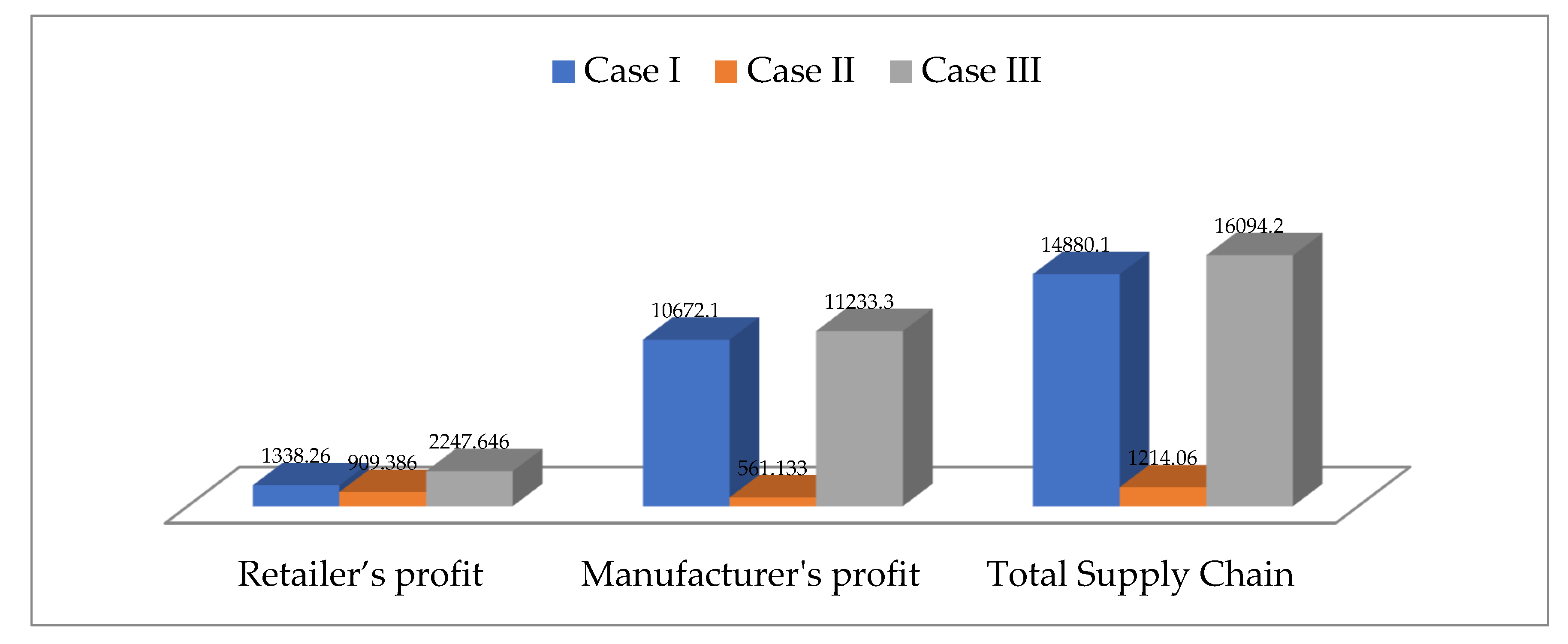
Obviously, Figure 4 presents the performance of offline policy less than mixture policy. It implied that the channel members would like to adopt new online technologies in a smaller, safe environment with the retailer and manufacturer before they scaled out to retail partners.
7.2. Sensitivity Analysis
To perform data analysis, the relative contributions of these parameters (, , , , , , , ) were calculated on the values of , , , and . Each parameter was adjusted separately by +50%, +25%, −25%, or −50%. Our analytical results are in Table 4.
7.3. The Discussion of Results
This section will compare and analyze the three contracts. The data analysis has highlighted a most interesting possibility: Reputation management and transportation performance. Several management implications can be drawn from Table 5. Marketing policies are changes in sales or other results that can be expected from a particular strategy. For example, ensuring food quality and security during the transportation and postponing strategy.
8. Conclusions
Due to the evolution of O2O technologies, the coordination mechanism will be incorporated into the classic inventory model. The authors develop a food supply chain among one manufacturer and one retailer under the O2O model in this research. The study also compared the three coordination mechanisms to fill the gap knowledge between theoretical and empirical in terms of inventory management. Relying on the existing theoretical results, this study has attempted to point out the optimal solution through examining decision-makers with an algorithm. Therefore, the authors can assert based on having understood the shortcomings of O2O technology that our theoretical claim about how a manufacturer and its compromising retailer evaluate a suitable ordering process through a comparison of three commitment contracts. Meanwhile, there are some potential bottlenecks in the development of the O2O model, including (1) users and offline sellers lack rational knowledge of mobile e-commerce; (2) the security of e-payments; and (3) the lack of innovations. Moreover, the findings have been proved by several examples to clarify the proposed model and solution. A total of the proof examples highlighted that (1) Mobile payment lays the foundation for online/offline integration strategy. With advancements in e-payment systems and face recognition/fingerprint recognition, both companies and consumers discover new technology to pay online quickly; (2) the IoT-Driven cold chain tracking is reducing logistics cost and improving business effectiveness, (3) Instant distribution impact on customer online satisfaction. Among the many topics to be explored in future research, some important ones are as follows: Estimating an effective after-seller’s services mechanism, strengthening consumers’ loyalty to offline sellers, and improving the innovative capacity of the O2O platform.
Author Contributions
Conceptualization, Y.-F.H. and N.X.; methodology, M.-W.W.; software, M.-W.W.; validation, Y.-F.H., N.X., M.-W.W., and M.-H.D.; formal analysis, N.X.; investigation, N.X.; resources, N.X.; data curation, N.X.; writing—original draft preparation, N.X., M.-W.W., and M.-H.D.; writing—review and editing, N.X., M.-W.W., and M.-H.D.; visualization, Y.-F.H.; supervision, Y.-F.H.; project administration, Y.-F.H. All authors have read and agreed to the published version of the manuscript.
Funding
This research received no external funding.
Institutional Review Board Statement
Not applicable.
Informed Consent Statement
Not applicable.
Data Availability Statement
Due to its proprietary nature <or ethical concerns>, supporting data cannot be made openly available. Further information about the data and conditions for access are available at http://www.xiongmaodangao.com/.
Acknowledgments
The authors would like to thank the editor and anonymous reviewers for their valuable and constructive comments, which have led to a significant improvement in the manuscript. The author’s research was partially supported by the Ministry of Science and Technology of the Republic of China under Grant MOST 109-2622-H-324-001.
Conflicts of Interest
The authors declare no conflict of interest.
Nomenclature
In addition: the following notations and assumptions are used throughout this article.
| System Parameters | |
| Retailer’s base demand. | |
| Manufacturer’s production rate, where . | |
| Manufacturer’s ordering cost per order. | |
| Manufacturer’s the setup cost per order. | |
| Self-price sensitivity. | |
| Cross-price sensitivity. | |
| Retailer’s price per unit offline. | |
| Retailer’s price per unit online. | |
| Goodwill cost of the manufacturer. | |
| Goodwill cost of the retailer, . | |
| Fixed costs per shipment. | |
| All-unit freight charged per unit. | |
| Retailer’s unit wholesale price, where . | |
| Manufacturer’s unit production cost. | |
| Retailer’s the marginal cost. | |
| Manufacturer’s holding cost per unit per unit time. | |
| Order quantity. | |
| Expected sales. | |
| Buy-back price of unsold items (paid by the manufacturer toward the retailer). | |
| New wholesale price. | |
| Wholesale price. | |
| Revenue-sharing fraction, . | |
| Quantity-flexibility fraction, . | |
| The ratio between the COP at the cooling temperature, set by the manufacturer for treating the product (i.e.). | |
| Total profit of the retailer during cycle time. | |
| Total profit of the manufacturer during production cycle. | |
| Decision Variables | |
| Optimal order quantity for supply chain coordination, . | |
| Number of shipments from the supplier to the retailer per production. | |
| Optimal temperature . | |
References
- Ma, J. 2017 Letter to Shareholders. 2017. Available online: https://medium.com/swlh/5-retail-insights-from-alibabas-new-retail-revolution-1855bc39bc64 (accessed on 7 December 2020).
- CNNIC. China’s Online Shopping Market Research Report in 2012. 2013. Available online: http://www.cnnic.cn/hlwfzyj/hlwxzbg/dzswbg/201304/t20130417_39290.htm (accessed on 7 December 2020).
- Du, R.; Jiang, J. New retailing: Connotation, development motivation and key issues. Price Theory Pract 2017, 2, 139–141. [Google Scholar]
- Maimaiti, M.; Zhao, X.; Jia, M.; Ru, Y.; Zhu, S. How we eat determines what we become: Opportunities and challenges brought by food delivery industry in a changing world in China. Eur. J. Clin. Nutr. 2018, 72, 1282–1286. [Google Scholar] [CrossRef] [PubMed]
- Chen, X.; Wang, X.; Jiang, X. The impact of power structure on the retail service supply chain with an O2O mixed channel. J. Oper. Res. Soc. 2016, 67, 294–301. [Google Scholar] [CrossRef]
- He, Z.; Cheng, T.C.E.; Dong, J.; Wang, S. Evolutionary location and pricing strategies for service merchants in competitive O2O markets. Eur. J. Oper. Res. 2016, 254, 595–609. [Google Scholar] [CrossRef]
- Smith, D.; Sparks, L. Temperature controlled supply chains. In Food Supply Chain Management; Blackwell Publishing: Oxford, UK, 2004; pp. 179–198. [Google Scholar]
- Van der Vorst, J.; Van Kooten, O.; Marcelis, W.J.; Luning, P.A.; Beulens, A.J.M. Quality controlled logistics in food supply chain networks: Integrated decision-making on quality and logistics to meet advanced customer demands. In Proceedings of the 14th International EurOMA Conference, Ankara, Turkey, 17–20 June 2007. [Google Scholar]
- Trienekens, J.; Zuurbier, P. Quality and safety standards in the food industry, developments and challenges. Int. J. Prod. Econ. 2008, 113, 107–122. [Google Scholar] [CrossRef]
- Zanoni, S.; Zavanella, L. Chilled or frozen? Decision strategies for sustainable food supply chains. Int. J. Prod. Econ. 2012, 140, 731–736. [Google Scholar] [CrossRef]
- Ahuja, R.K.; Huang, W.; Romeijn, H.E.; Morales, D.R. A heuristic approach to the multi-period single-sourcing problem with production and inventory capacities and perishability constraints. INFORMS J. Comput. 2007, 19, 14–26. [Google Scholar] [CrossRef] [Green Version]
- Mercier, S.; Villeneuve, S.; Mondor, M.; Uysal, I. Time-Temperature Management Along the Food Cold Chain: A Review of Recent Developments. Compr. Rev. Food Sci. Food Saf. 2017, 16, 647–667. [Google Scholar] [CrossRef]
- Lu, C.J.; Lee, T.S.; Gu, M.; Yang, C.T. A multistage sustainable production-inventory model with carbon emission reduction and price-dependent demand under stackelberg game. Appl. Sci. 2020, 10, 4878. [Google Scholar] [CrossRef]
- Kelepouris, T.; Pramatari, K.; Doukidis, G. RFID-enabled traceability in the food supply chain. Ind. Manag. Data Syst. 2007, 107, 183–200. [Google Scholar] [CrossRef]
- Manzini, R.; Accorsi, R. The new conceptual framework for food supply chain assessment. J. Food Eng. 2013, 115, 251–263. [Google Scholar] [CrossRef]
- Yu, M.; Nagurney, A. Competitive food supply chain networks with application to fresh produce. Eur. J. Oper. Res. 2013, 224, 273–282. [Google Scholar] [CrossRef]
- Gouda, S.K.; Saranga, H. Sustainable supply chains for supply chain sustainability: Impact of sustainability efforts on supply chain risk. Int. J. Prod. Res. 2018, 56, 5820–5835. [Google Scholar] [CrossRef]
- Goyal, S.K. An integrated inventory model for a single supplier-single customer problem. Int. J. Prod. Res. 1977, 15, 107–111. [Google Scholar] [CrossRef]
- Darwish, M.; Odah, O.M. Vendor managed inventory model for single-vendor multi-retailer supply chains. Eur. J. Oper. Res. 2010, 204, 473–484. [Google Scholar] [CrossRef]
- Lin, Y.J.; Ouyang, L.Y.; Dang, Y.F. A joint optimal ordering and delivery policy for an integrated supplier–retailer inventory model with trade credit and defective items. Appl. Math. Comput. 2012, 218, 7498–7514. [Google Scholar] [CrossRef]
- Ouyang, L.Y.; Ho, C.H.; Su, C.H.; Yang, C.T. An integrated inventory model with capacity constraint and order-size dependent trade credit. Comput. Ind. Eng. 2015, 84, 133–143. [Google Scholar] [CrossRef]
- Vijayashree, M.; Uthayakumar, R. A single-vendor and a single-buyer integrated inventory model with ordering cost reduction dependent on lead time. J. Ind. Eng. Int. 2017, 13, 393–416. [Google Scholar] [CrossRef] [Green Version]
- Pang, Q.; Chen, Y.; Hu, Y. Coordinating three-level supply chain by revenue-sharing contract with sales effort dependent demand. Discrete. Dyn. Nat. Soc. 2014, 2014, 561081. [Google Scholar] [CrossRef] [Green Version]
- Tsao, Y.C.; Lee, P.L. Employing revenue sharing strategies when confronted with uncertain and promotion-sensitive demand. Comput. Ind. Eng. 2020, 139, 106200. [Google Scholar] [CrossRef]
- Zhao, X.; Wu, F. Coordination of agri-food chain with revenue-sharing contract under stochastic output and stochastic demand. Asia-Pac. J. Oper. 2011, 28, 487–510. [Google Scholar] [CrossRef]
- Cachon, G.P.; Lariviere, M.A. Supply chain coordination with revenue-sharing contracts: Strengths and limitations. Manag. Sci. 2005, 51, 30–44. [Google Scholar] [CrossRef] [Green Version]
- Sang, S. Revenue sharing contract in a multi-echelon supply chain with fuzzy demand and asymmetric information. Int. J. Comput. Int. Sys. 2016, 9, 1028–1040. [Google Scholar] [CrossRef] [Green Version]
- Yao, Z.; Leung, S.C.H.; Lai, K.K. The effectiveness of revenue-sharing contract to coordinate the price-setting newsvendor products’ supply chain. Supply Chain. Manag. 2008, 13, 263–271. [Google Scholar] [CrossRef]
- Govindan, K.; Malomfalean, A. A framework for evaluation of supply chain coordination by contracts under O2O environment. Int. J. Prod. Econ. 2019, 215, 11–23. [Google Scholar] [CrossRef]
- Gong, Q. Optimal buy-back contracts with asymmetric information. Int. J. Manag. Mark. Res. 2008, 1, 23–47. [Google Scholar]
- Wang, Y.; Zipkin, P. Agents’ incentives under buy-back contracts in a two-stage supply chain. Int. J. Prod. Econ. 2009, 120, 525–539. [Google Scholar] [CrossRef]
- Hou, J.; Zeng, A.Z.; Zhao, L. Coordination with a backup supplier through buy-back contract under supply disruption. Transp. Res. E Logist. Transp. Rev. 2010, 46, 881–895. [Google Scholar] [CrossRef]
- Ding, X.S.; Zhang, J.H.; Chen, X. A joint pricing and inventory control problem under an energy buy-back program. Oper. Res. Lett. 2012, 40, 516–520. [Google Scholar] [CrossRef]
- Tibrewala, R.; Tibrewala, R.; Meena, P.L. Buy-back policy for supply chain coordination: A simple rule. Int. J. Oper. Res. 2012, 31, 1–28. [Google Scholar] [CrossRef]
- Zhang, L.H.; Li, T.; Fan, T.J. Inventory misplacement and demand forecast error in the supply chain: Profitable RFID strategies under wholesale and buy-back contracts. Int. J. Prod. Res. 2018, 56, 5188–5205. [Google Scholar] [CrossRef]
- Dai, T.; Li, Z.; Sun, D. Equity-based incentives and supply chain buy-back contracts. Decis. Sci. J. 2012, 43, 661–686. [Google Scholar] [CrossRef]
- Sainathan, A.; Groenevelt, H. Vendor managed inventory contracts-coordinating the supply chain while looking from the vendor’s perspective. Eur. J. Oper. Res. 2019, 272, 249–260. [Google Scholar] [CrossRef]
- Tsay, A.; Lovejoy, W.S. Quantity flexibility contracts and supply chain performance. Manuf. Serv. Oper. Manag. 1999, 1, 89–111. [Google Scholar] [CrossRef]
- Li, C.L.; Kouvelis, P. Flexible and risk-sharing supply contracts under price uncertainly. Manag. Sci. 1999, 45, 1378–1398. [Google Scholar] [CrossRef]
- Sethi, S.; Yan, H.; Zhang, H. Quantity flexibility contracts: Optimal decisions with information updates. Decis. Sci. 2004, 35, 691–712. [Google Scholar] [CrossRef]
- Wu, J. Quantity flexibility contracts under Bayesian updating. Comput. Oper. Res. 2005, 32, 1267–1288. [Google Scholar] [CrossRef]
- Milner, J.M.; Kouvelis, P. Order quantity and timing flexibility in supply chains: The role of demand characteristics. Manag. Sci. 2005, 51, 970–985. [Google Scholar] [CrossRef] [Green Version]
- Bag, S.; Chakraborty, D.; Roy, A.R. A production inventory model with fuzzy random demand and with flexibility and reliability considerations. Comput. Ind. Eng. 2009, 56, 411–416. [Google Scholar] [CrossRef]
- Li, X.; Lian, Z.; Choong, K.K.; Liu, X. A quantity-flexibility contract with coordination. Int. J. Prod. Econ. 2016, 179, 273–284. [Google Scholar] [CrossRef]
- Lian, Z.; Deshmukh, A. Analysis of supply contracts with quantity flexibility. Eur. J. Oper. Res. 2009, 196, 526–533. [Google Scholar] [CrossRef]
- Aung, M.M.; Chang, Y.S. Temperature management for the quality assurance of a perishable food supply chain. Food. Control. 2014, 40, 198–207. [Google Scholar] [CrossRef]
- Lorite, G.S.; Selkälä, T.; Siploa, T.; Palenzuela, J.; Jubete, E.; Viñuales, A.; Cabañero, G.; Grande, H.J.; Tuominen, J.; Uusitalo, S.; et al. Novel, smart and RFID assisted critical temperature indicator for supply chain monitoring. J. Food Eng. 2017, 193, 20–28. [Google Scholar] [CrossRef] [Green Version]
- Kuo, J.C.; Chen, M.C. Developing an advanced multi-temperature joint distribution system for the food cold chain. Food. Control. 2010, 21, 559–566. [Google Scholar] [CrossRef]
- Lawrence, J.J.; Pasternack, B.A. Applied Management Science: Modeling, Spreadsheet Analysis, and Communication for Decision Making, 2nd ed.; Wiley: New York, NY, USA, 2002. [Google Scholar]
- Aksen, D. Loss of customer goodwill in the uncapacitated lot-sizing problem. Comput. Oper. Res. 2007, 34, 2805–2823. [Google Scholar] [CrossRef]
- Finn, Z.S.; Anderson, T.; Lund, D. Spoiled brands: Protecting your company’s goodwill and assets from food contamination claims. CPCU eJournal 2008, 61, 1–8. [Google Scholar]
- Mitreva, E.; Gjurevska, S. The need for a quality system in a company for bread and bakery production in Macedonia. Quality 2018, 19, 118–124. [Google Scholar]
- Hobbs, J.E. Food supply chains during the COVID-19 pandemic. Can. J. Agric. Econ. 2020, 68, 171–176. [Google Scholar] [CrossRef] [Green Version]
- Singh, S.; Kumar, R.; Panchal, R.; Tiwari, M.K. Impact of COVID-19 on logistic systems and disruptions in food supply chain. Int. J. Prod. Res. 2020, 1–16. [Google Scholar] [CrossRef]
- Rizou, M.; Galanakis, J.M.; Aldawoud, T.M.S.; Galanakis, C.M. Safety of foods, food supply chain and environment within the COVID-19 pandemic. Trends Food Sci. Technol. 2020, 102, 293–299. [Google Scholar] [CrossRef] [PubMed]
- He, Z.; Han, G.; Cheng, T.C.E.; Fan, B.; Dong, J. Evolutionary food quality and location strategies for restaurants in competitive online-to-offline food ordering and delivery markets: An agent-based approach. Int. J. Prod. Econ. 2019, 215, 61–72. [Google Scholar] [CrossRef]
- Wang, O.; Somogyi, S.; Charlebois, S. Food choice in the e-commerce era a comparison between business-to-consumer (B2C), online-to-offline (O2O) and new retail. Br. Food J. 2020, 122, 1215–1237. [Google Scholar] [CrossRef]
- Li, C.; Mirosa, M.; Bremer, P. Review of online food delivery platforms and their impacts on sustainability. Sustainability 2020, 12, 5528. [Google Scholar] [CrossRef]
- Yang, C.T.; Ho, C.H.; Lee, H.M.; Ouyang, L.Y. Supplier-retailer production and inventory models with defective items and inspection errors in non-cooperative and cooperative environments. RAIRO-Oper. Res. 2018, 52, 453–471. [Google Scholar] [CrossRef]
- Peleg, M.; Engel, R.; Gonzalez-Martinez, C.; Corradini, M.G. Non-Arrhenius and non-WLF kinetics in food systems. J. Sci. Food Agric. 2002, 82, 1346–1355. [Google Scholar] [CrossRef]
- Rong, A.; Akkerman, R.; Grunow, M. An optimization approach for managing fresh food quality throughout the supply chain. Int. J. Prod. Econ. 2011, 131, 421–429. [Google Scholar] [CrossRef]
- Chen, L.; Kou, M.; Wang, S. On the use of importance measures in the reliability of inventory systems, considering the cost. Appl. Sci. 2020, 10, 7942. [Google Scholar] [CrossRef]
Figure 1.
New retailing business model.
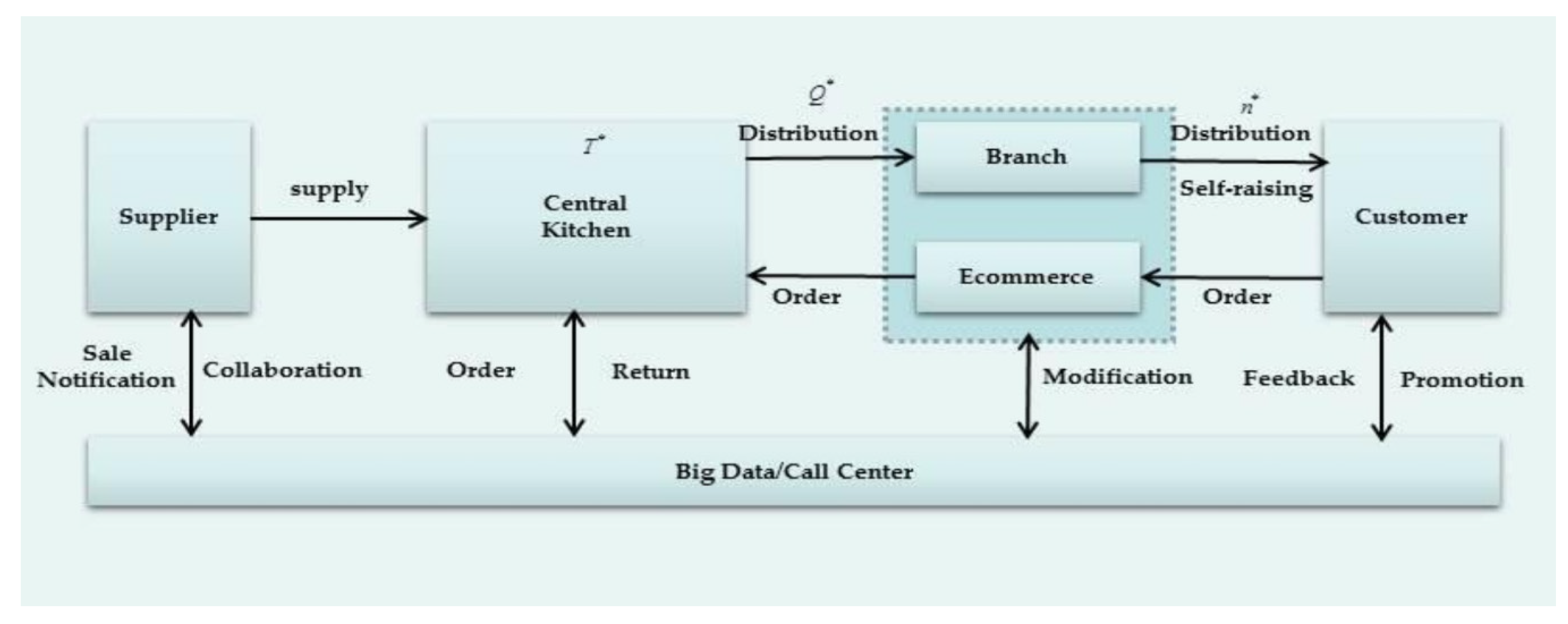
Figure 2.
Cake supply chain summary.
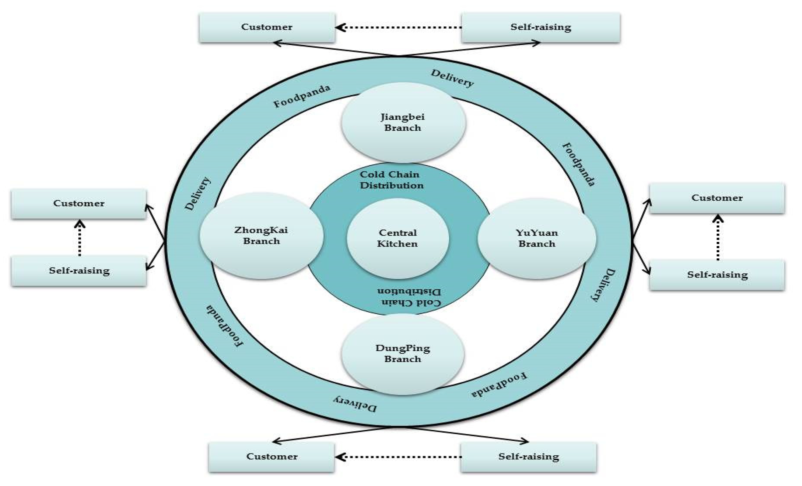
Figure 3.
Mixture situation measures under three policies.
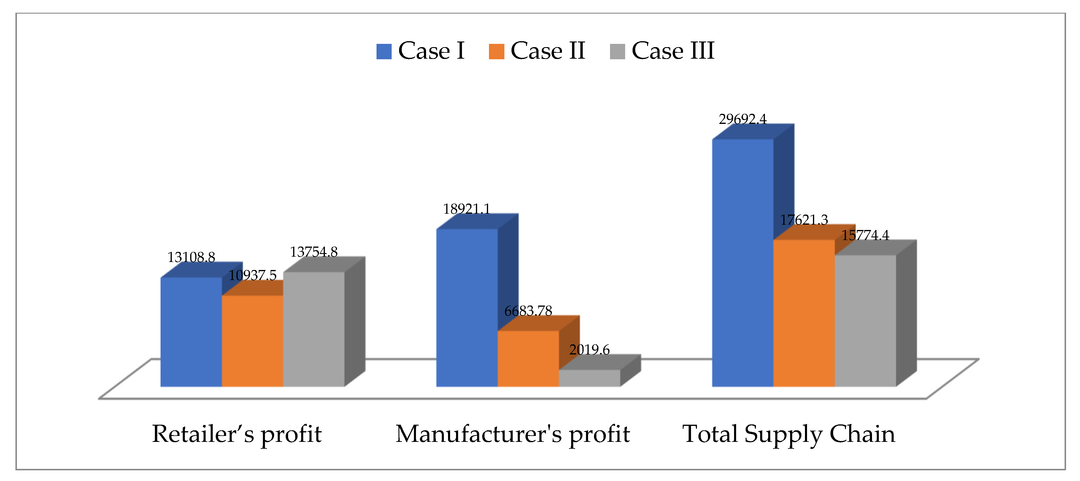
Figure 4.
Offline situation measures under three policies.

Table 1.
The main classification of inventory models from relevant studies.
| Reference | Model | Demand | Revenue-Sharing Contract | Buy-Back Contract | Quantity-Flexibility Contract |
|---|---|---|---|---|---|
| Pang et al. [23] | Supply chain | Sales effort dependent | V | ||
| Tsao & Lee [24] | Supply chain | Uncertain and promotion-sensitive | V | ||
| Zhao & Wu [25] | Stochastic | V | |||
| Cachon & Lariviere [26] | Supply chain | Price-dependent | V | ||
| Sang [27] | Supply chain | Fuzzy demand | V | ||
| Yao et al. [28] | Supply chain | Price-dependent demand | V | ||
| Govindan & Malomfalean [29] | Supply chain | Constant | V | V | V |
| Gong [28] | Supply chain | Stochastic | V | ||
| Wang & Zipkin [30] | Supply chain | Constant | V | ||
| Hou et al. [32] | Supply chain | Constant | V | ||
| Ding et al. [33] | EOQ | Price-dependent demand | V | ||
| Tibrewala et al. [34] | Supply chain | Stochastic | V | ||
| Zhang et al. [35] | Supply chain | Stochastic | V | ||
| Dai et al. [36] | Supply chain | Stochastic | V | ||
| Sainathan & Groenevelt [37] | Supply chain | Constant | V | V | V |
| Tsay & Lovejoy [38] | Supply chain | Stochastic | V | ||
| Li & Kouvelis [39] | Supply chain | Constant | V | V | |
| Sethi et al. [40] | Supply chain | Stochastic | V | ||
| Wu [41] | Supply chain | Stochastic | V | ||
| Milner & Kouvelis [42] | Supply chain | Stochastic | V | ||
| Bag et al. [43] | EPQ | Stochastic | V | ||
| Li et al. [44] | Supply chain | Constant | V | ||
| Lian & Deshmukh [45] | Supply chain | Stochastic | V | ||
| Present article | Food supply chain | Constant | V | V | V |
Table 2.
The value of parameters for Example 1. with new retailing problem.
| = 1000 | = 2000 | = 9 | = 170 |
| = 160 | = 0.1 | = 80 | = $10 |
| = $5 | = $8 | = $0.1 | = $5 |
| = $15 | = $1 | = 0.55 | = 0.4 |
| = 6 | = 5 | = 40 | = 100 |
| = 0.5 | = $4 | ||
Table 3.
Computation results of Example 1. for online and offline.
| Online + Offline | Case I | Case II | Case III |
|---|---|---|---|
| 46.3743 | 45.3534 | 47.8674 | |
| 2.4070 | 2.29413 | 2.30921 | |
| 32 | 32 | 10 | |
| TPB | 13,108.8 | 10,937.5 | 13,754.8 |
| TPFck | 18,921.1 | 6683.78 | 2019.6 |
| TP | 29,692.4 | 17,621.3 | 15,774.4 |
| Offline | Case I | Case II | Case III |
| 42.1495 | 43.634 | 46.8146 | |
| 2.29675 | 2.34995 | 2.38194 | |
| 30 | 30 | 12 | |
| TPB | 1338.26 | 10,672.1 | 14,880.1 |
| TPFck | 909.386 | 561.133 | 1214.06 |
| TP | 2247.646 | 11233.3 | 16,094.2 |
Table 4.
Effect of changes in various parameters of the model.
| Para. | % | CASE I | CASE II | CASE III | |||
|---|---|---|---|---|---|---|---|
| −50% | (46.54, 2.61, 34) | (13,005.1, 20, 060.3) | (45.89, 2.21, 32) | (10, 955.2, 7439.55) | (48.14, 2.43, 10) | (11,692.5, 2123.1) | |
| −25% | (46.42, 2.59, 33) | (13,098.2, 19, 661.3) | (45.86, 2.22, 32) | (10, 945.1, 7223.54) | (48.02, 2.36, 10) | (12,991.3, 2117.9) | |
| 0 | (46.37, 2.40, 32) | (13,108.8, 18, 921.1) | (45.35, 2.29, 32) | (10, 937.5, 6683.78) | (47.86, 2.30, 10) | (13,754.8, 2019.6) | |
| 25% | (46.32, 2.39, 32) | (14,098.2, 18, 842.2) | (43.83, 2.36, 32) | (10, 627.5, 6791.53) | (42.78, 2.26, 10) | (17,128.4, 2007.1) | |
| 50% | (46.28, 2.38, 32) | (14,099.3, 18, 432.7) | (43.80, 2.36, 32) | (10, 628.5, 6975.53) | (42.66, 2.21, 10) | (17,195.0, 2001.6) | |
| −50% | (46.44, 2.56, 32) | (14,740.1, 19, 253.6) | (46.49, 2.27, 32) | (17, 035.2, 7043.44) | (48.50, 2.29, 10) | (17,115.6, 1921.5) | |
| −25% | (46.41, 2.49, 32) | (14,418.5, 19, 252.7) | (46.16, 2.27, 32) | (13, 830.6, 7025.41) | (48.20, 2.29, 10) | (13,910.8, 1940.4) | |
| 0 | (46.37, 2.40, 32) | (13,108.8, 18, 921.1) | (45.35, 2.29, 32) | (10, 937.5, 6683.78) | (47.86, 2.30, 10) | (13,754.8, 2019.6) | |
| 25% | (46.33, 2.38, 32) | (9775.51, 18,250.9) | (43.53, 2.43, 32) | (7421.73, 6989.81) | (-,-,-) | (-,-) | |
| 50% | (46.29, 2.31, 32) | (9454.01, 18,250.1) | (43.22, 2.44, 32) | (4217.41, 6972.22) | (-,-,-) | (-,-) | |
| −50% | (46.37, 2.40, 32) | (14,102.1, 18,921.1) | (45.35, 2.29, 32) | (10,851.1, 6683.78) | (-,-,-) | (-,-) | |
| −25% | (46.37, 2.40, 32) | (13,099.5, 18,921.1) | (45.35, 2.29, 32) | (10,854.5, 6683.78) | (-,-,-) | (-,-) | |
| 0 | (46.37, 2.40, 32) | (13,108.8, 18,921.1) | (45.35, 2.29, 32) | (10,937.5, 6683.78) | (-,-,-) | (-,-) | |
| 25% | (46.37, 2.40, 32) | (10,094.5, 18,921.1) | (45.35, 2.29, 32) | (11,149.5, 6683.78) | (-,-,-) | (-,-) | |
| 50% | (46.37, 2.40, 32) | (10,092.1, 18,921.1) | (45.35, 2.29, 32) | (11,172.1, 6683.78) | (-,-,-) | (-,-) | |
| −50% | (47.67, 2.43, 32) | (13,184.3, 19,282.1) | (45.93, 2.40, 32) | (10,976.9, 7067.72) | (-,-,-) | (-,-) | |
| −25% | (47.00, 2.41, 32) | (13,140.2, 19,267.1) | (45.38, 2.40, 32) | (10,951.4, 7037.41) | (-,-,-) | (-,-) | |
| 0 | (46.37, 2.40, 32) | (13,108.8, 18,921.1) | (45.35, 2.29, 32) | (10,937.5, 6683.78) | (-,-,-) | (-,-) | |
| 25% | (45.76, 2.09, 33) | (10,054.8, 18,236.4) | (43.33, 2.29, 33) | (10,901.1, 6678.07) | (-,-,-) | (-,-) | |
| 50% | (45.17, 1.93, 33) | (10,013.4, 18,220.9) | (40.38, 2.29, 33) | (10,820.5, 6596.76) | (-,-,-) | (-,-) | |
| −50% | (48.50, 2.33, 31) | (13,238.7, 19,299.7) | (45.83, 2.46, 31) | (10,977.9, 6604.68) | (-,-,-) | (-,-) | |
| −25% | (47.40, 2.38, 32) | (13,166.6, 19,276.1) | (45.71, 2.45, 31) | (10,966.7, 6655.55) | (-,-,-) | (-,-) | |
| 0 | (46.37, 2.40, 32) | (13,108.8, 18,921.1) | (45.35, 2.29, 32) | (10,937.5, 6683.78) | (-,-,-) | (-,-) | |
| 25% | (45.41, 2.45, 33) | (10,029.9, 18,227.2) | (43.03, 2.26, 32) | (10,586.2, 6960.57) | (-,-,-) | (-,-) | |
| 50% | (44.50, 2.47, 34) | (9964.94, 18,202.2) | (42.25, 2.21, 32) | (10,546.9, 6914.61) | (-,-,-) | (-,-) | |
| −50% | (46.56, 2.30, 32) | (10,081.7, 19,590.1) | (45.35, 2.29, 32) | (10,937.5, 6683.78) | (-,-,-) | (-,-) | |
| −25% | (46.44, 2.31, 32) | (10,064.3, 19,580.8) | (45.35, 2.29, 32) | (10,937.5, 6683.78) | (-,-,-) | (-,-) | |
| 0 | (46.37, 2.40, 32) | (13,108.8, 18,921.1) | (45.35, 2.29, 32) | (10,937.5, 6683.78) | (-,-,-) | (-,-) | |
| 25% | (46.28, 2.42, 32) | (13,139.9, 18,912.4) | (45.35, 2.29, 32) | (10,937.5, 6683.78) | (-,-,-) | (-,-) | |
| 50% | (46.19, 2.43, 32) | (13,182.9, 18,872.9) | (45.35, 2.29, 32) | (10,937.5, 6683.78) | (-,-,-) | (-,-) | |
| −50% | (43.85, 0.07, 34) | (13,626.1, 17,007.4) | (45.35, 0.06,34) | (10,626.1, 7007.54) | (-,-,-) | (-,-) | |
| −25% | (43.85, 1.07, 33) | (13,626.1, 17,007.4) | (45.35, 1.06,34) | (10,626.1, 7007.54) | (-,-,-) | (-,-) | |
| 0 | (46.37, 2.41, 32) | (13,108.8, 18,921.1) | (45.35, 2.29,32) | (10,937.5, 6683.78) | (-,-,-) | (-,-) | |
| 25% | (-,-,-) | (-,-) | (-,-,-) | (-,-) | (-,-,-) | (-,-) | |
| 50% | (-,-,-) | (-,-) | (-,-,-) | (-,-) | (-,-,-) | (-,-) | |
| −50% | 26.3743 | (10,069.1, 6335.23) | (26.37, 0.67, 32) | (10,069.1, 7335.23) | (-,-,-) | (-,-) | |
| −25% | 43.8481 | (10,626.1, 7007.54) | (43.84, 1.53, 32) | (10,626.1, 7007.54) | (-,-,-) | (-,-) | |
| 0 | 46.3743 | (13,108.8, 18,921.1) | (45.35, 2.29, 32) | (10,937.5, 6683.78) | (-,-,-) | (-,-) | |
| 25% | (-,-,-) | (-,-) | (-,-,-) | (-,-) | (-,-,-) | (-,-) | |
| 50% | (-,-,-) | (-,-) | (-,-,-) | (-,-) | (-,-,-) | (-,-) | |
Note: Para. = Parameter; % = Change %.
Table 5.
Effect of changes in various parameters of managerial insights.
| Increasing Parameter(s) | Case I | Case II | Case III |
|---|---|---|---|
| Company’s goodwill is an intangible asset owned by and associated with operation of a company. Thus, a trademark is often an important investment in protecting the intellectual property of a manufacturer. | More specifically, in a high critical ratio environment revenue sharing contracts are more profitable for the manufacturer than buyback contracts. | With goodwill cost exists, the channel coordination provides allocation of the supply chain’s profit if . | |
| The contract offers accepted by the retailer, two-part tariff and quantity discount increases the efficiency of the channel in the terms of channel profit. | The contract provides an enormous motivation for retailer to give orders more than usual without concerning stock out in inventory. | With goodwill cost exists, the channel coordination provides allocation of the supply chain’s profit if . | |
| The online retailer provides the freight subsidy to the manufacturer increase the profit of the total profit. | Allows a retailer to return unsold inventory up to a specified amount at an agreed upon price/freight fee, resulting in higher product availability and higher profits for both the retailer and the manufacturer. | ||
| A wholesale price is plausibly below transportation fee, the members may have adopted a coordinating contract. | Focusing on the transportation costs. The retailer and the manufacturer will be covering the transportation cost. | ||
| If , which a wholesale price is greater than marginal cost, which is in sharp contrast to the optimal wholesale price under a revenue-sharing contract. | The manufacturer would like to increase his own profit by increasing the wholesale price and buy-back price, where , . | ||
| With revenue-sharing fraction, the manufacturer willingly reduces its wholesale price and makes money by sharing the retailer’s revenue. | If effort is significant (i.e., ), the effect dominates the quantity effect, and the wholesale price falls. | ||
| To monitor the food quality in the distribution, the absolute temperature decreased by a coefficient of , the manufacturer will increase the channel profit. | To monitor the food quality in the distribution, the absolute temperature decreased by a coefficient of , the manufacturer will increase the channel profit. | ||
| To monitor the food quality in the distribution, the absolute temperature decreased by a coefficient of , the manufacturer will increase the channel profit. | To monitor the food quality in the distribution, the absolute temperature decreased by a coefficient of , the manufacturer will increase the channel profit. |
Publisher’s Note: MDPI stays neutral with regard to jurisdictional claims in published maps and institutional affiliations. |
© 2021 by the authors. Licensee MDPI, Basel, Switzerland. This article is an open access article distributed under the terms and conditions of the Creative Commons Attribution (CC BY) license (http://creativecommons.org/licenses/by/4.0/).
Share and Cite
MDPI and ACS Style
Xu, N.; Huang, Y.-F.; Weng, M.-W.; Do, M.-H. New Retailing Problem for an Integrated Food Supply Chain in the Baking Industry. Appl. Sci. 2021, 11, 946. https://doi.org/10.3390/app11030946
AMA Style
Xu N, Huang Y-F, Weng M-W, Do M-H. New Retailing Problem for an Integrated Food Supply Chain in the Baking Industry. Applied Sciences. 2021; 11(3):946. https://doi.org/10.3390/app11030946
Chicago/Turabian StyleXu, Ning, Yung-Fu Huang, Ming-Wei Weng, and Manh-Hoang Do. 2021. "New Retailing Problem for an Integrated Food Supply Chain in the Baking Industry" Applied Sciences 11, no. 3: 946. https://doi.org/10.3390/app11030946
Note that from the first issue of 2016, this journal uses article numbers instead of page numbers. See further details here.