Detection of Density Changes in Soils with Impedance Spectroscopy


1
Institute for Measurement Engineering and Sensor Technology, Ruhr West University of Applied Sciences, 45479 Mülheim an der Ruhr, Germany
2
Chair for Measurement and Sensor Technology, Chemnitz University of Technology, 09126 Chemnitz, Germany
*
Author to whom correspondence should be addressed.
Appl. Sci. 2021, 11(4), 1568; https://doi.org/10.3390/app11041568
Submission received: 17 December 2020
/
Revised: 1 February 2021
/
Accepted: 3 February 2021
/
Published: 9 February 2021
(This article belongs to the Special Issue Impedance Spectroscopy and Its Application in Measurement and Sensor Technology)
Abstract
:Measurement of soil parameters, such as moisture, density and density change, can provide important information for evaluating the stability of earthwork structures and for structural health monitoring. To ensure the stability of flood protection dikes, erosion at the contact zones of different soil zones must be avoided. In this work we propose the use of impedance spectroscopy to measure changes in density and volume caused by contact erosion. Erosion leads generally to a volume decrease in the contact zones between soils with different grain sizes and, consequently, to cavities in the dike structure. For this purpose, a proctor mould was developed for emulating contact erosion and the realisation of impedance measurements. Experimental investigations show a correlation between volume change of the soils in the proctor mould and impedance value. For a volume change of soil in the range of approximately 1.5% to 5.3%, an impedance change arises in the range of 17.2% to 29.8%. With several investigations we proof, that it is possible to detect material transport by impedance spectroscopy.
1. Introduction
Due to anthropogenic climate change, flood events are statistically increasing worldwide. Therefore, technical flood protection measurements, a core task for ensuring civil security, have become acutely important in recent years. Examples include the construction of new flood protection polders along the Rhine River, or the inspection and maintenance of existing flood protection structures. Within the framework of the stability analyses of dikes, it has to be demonstrated that there is sufficient safety against contact erosion and suffosion between the individual dike zones and layers. In geological terminology, the phenomena of contact erosion and suffosion, in which material transport of the finer soil into the coarser soil takes place at a transition between two soil layers, are summarised under the term material transport. In addition, the phenomena of hydraulic ground failure and regressing erosion ground failure are also included but are not the primary focus of this work. Since the current criteria for avoiding erosion [1] have been determined empirically and are not applicable in many cases, a very conservative approach is often taken during planning. This can lead to inefficient and uneconomic designs. From both engineering and user’s points of view, it would therefore be desirable not only to estimate the empirical behaviour of contact erosion and suffosion, but also to be able to test material transport characteristics in a laboratory setting. This would allow for project-related assessments of the material transport risk.
To achieve this aim, a measuring method for detecting and monitoring density changes in soils has to be developed. This measuring method should be suitable for both laboratory evaluations in the planning phase of projects as well as in new or existing dikes as a monitoring system at known structural weak points, such as bends.
1.1. Impedance Spectroscopy
Electrical impedance spectroscopy is an established method for the characterisation of materials. The high information content in the frequency-dependent real part and imaginary part of the impedance can be used to determine various quantities that cannot be measured directly with regard to material interfaces, geometric structures and electrical and dielectric properties.
To measure the impedance spectrum, the real part and imaginary part of the impedance of a sample are measured at several frequencies. In principle, the evaluation can be carried out using mathematical and physical methods. With physical methods, the impedance spectra are modelled with equivalent circuit diagrams that were developed based on physical/chemical considerations. The desired information can be determined from the parameters of the equivalent circuit diagram using methods of complex, non-linear optimisation. This principle is already used in the determination of soil moisture and is now to be adapted to the measurement of density [2]. It was thereby proven that the impedance spectra include information about both soil composition and water content. In this paper, we base our investigation on these results and focus on the aspect of the ability of the method to provide information specifically on soil density. We propose to determine the density or density change by measuring the complex dielectric constant of the soil followed by density calculation based on an equivalent circuit model.
1.2. Structure of Dikes
Dikes are separated into several zones. Each of these zones has a specific function and is made of a different soil. Even though a dike has the function of retaining water, there is always a leakage caused by the porosity of the soils. The core of a dike consists of a material with a low water permeability, and as such, fine-grained materials like sand are usually applied for this purpose. On the dry side of a dike, there is a drain to allow the seepage water to drain away. This consists of a coarser-grained material. Between core and drain, there is a filter. The drain and filter are often combined within one zone. The filter is supposed to ensure that the fine-grained material of the core is not flushed into the drain. Therefore, it is important that contact erosion does not occur at the boundary layer between core and filter. For this purpose, the grain sizes of the two materials must be adjusted accordingly, taking into account the potential hydraulic gradient of the water [3].
1.3. Contact Erosion
Contact erosion is a form of internal erosion and, besides overtopping, the most common cause of dike failure. Contact erosion occurs at the boundary layer of two materials with different grain sizes. Driven by water flow, the finer material migrates into the pores of the coarser material (Figure 1). Material is transported if the hydraulic gradient (i.e., the ratio between pressure height difference and flow length) is large enough, and the difference in the grain size of the two materials allows this geometrically. The larger the difference in grain size and the higher the hydraulic gradient, the more likely that contact erosion is to occur [1,4,5].
1.4. State-of-the-Art Techniques
Ground-penetrating radar (GPR) is based on radar technology with frequencies of 10–1000 MHz [6]. The frequency influences the measurement depth and resolution. Low frequencies offer a large measurement depth but have low resolution. High frequencies offer a higher resolution but a correspondingly lower penetration depth into materials. The measuring effect is based on the travel time of electromagnetic waves in different materials, which is mainly influenced by their permittivity. Due to the resulting differing travel times of waves in different materials, conclusions can be made about the ground conditions [7].
GPR can be used in many areas of geotechnics. Common applications are the investigation of the composition of soil near the surface, the detection of cavities or sinkholes and the inspection of foundations and roads [6]. However, GPR has also been used to detect erosion processes in dams. This requires two drill holes for transmitter and receiver. With this arrangement, a tomogram of the dam can be recorded, which can then be used to detect erosion [8].
GPR is not suitable for the planned application, because a measurement takes too long and boreholes are necessary. Even though it can be used to detect defects, it is not ideal for monitoring. Thus, it is not applicable for the planned laboratory evaluations.
Another system for monitoring soil densities is the thermo-time domain reflectometry (T-TDR) [9,10,11]. This method combines the TDR technique with a heat pulse, which is used to determine the heat capacity and thermal conductivity of the soil. The heat impulse is emitted by one electrode, while the temperature change is measured over a distance by a second electrode. The heat capacity and thermal conductivity of the material can be determined using the known distance between the electrodes and the measured temperature increase. Moreover, TDR is utilised to determine the electrical conductivity of the material. Based on these three parameters, the density can be calculated.
This method offers the advantage of non-destructive density measurement and monitoring. The measuring range is limited to the material between the electrodes, and the results become more accurate with increasing electrode length. If water flow in the measuring range is too strong, the heat dissipates through the flow and the measurement is distorted. Since this is the case for dikes in critical areas and also for the newly developed test cell for laboratory evaluations, this measuring method is not suitable for this application.
A further method uses impedance spectroscopy in a soil density gauge system to determine soil characteristics such as soil density and soil moisture [12]. It consists of a transmitter electrode surrounded by a second ring-shaped receiver electrode. The flat electrodes are thereby placed on the material, and the impedance is measured between the two electrodes. The impedance spectrum is then used to determine the dielectric properties of the soil. Based on this, the soil density and moisture are determined. A comparison with a nuclear density meter [13], which is a reference measuring method for density and moisture of soils, shows some disadvantages of the system [14]. A complex calibration with a known soil type, which must have similar properties to the measured soil, is needed. Therefore, a second measuring device is needed to carry out a field calibration. However, even after calibration, a large deviation of the density measurement remains, depending on the soil moisture.
A known method for measuring soil moisture is impedance spectroscopy, whereby soil moisture is determined based on the dielectric constant of the soil [2]. To measure the impedance spectrum, two electrodes are positioned in the soil. When the water content changes, so does the dielectric constant, and therefore the impedance of the soil changes. Given that this is a static measurement, it is assumed that the soil composition does not change during the measurement. This would otherwise cause an additional change in the electrical properties of the soil, which would distort the measurement. With the help of system identification, a parameter extraction is carried out from the impedance spectrum in order to make conclusions about the water content of the soil. By reversing the principle and assuming that the soil is always completely saturated with water during an erosion process, the impedance can be used to infer changes in soil density. In this way, this measuring method could also be applied to measure density or density changes.
2. Materials and Methods
2.1. Dielectric Properties of Soils
Water and sediment have different dielectric properties. Freshwater has a relative dielectric constant (εr) of 81, and sediment is in the range of 2–10, depending on the soil type [2]. In an earthwork, such as a dike, sand and gravel, which have an εr of 4, are usually used as core. Completely saturated gravel–water and sand–water mixtures, therefore, have different dielectric properties. Due to the larger grain sizes of gravel, there is more water in the same volume than in a sand–water mixture. Therefore, εr is higher in a gravel–water mixture than in a sand–water mixture. In case of an erosion process, it can be assumed that the soil is completely saturated with water. During the erosion process, the sand migrates into the pores of the gravel and thus displaces the water. This effect leads to a change in εr. εr of the mixture can be described with the mixture model of Looyenga [15]. This was developed for mixing two material phases. Assuming that gravel and sand have the same εr, it can also be used in this case.
In the equation above, is the resulting relative dielectric constant, is the dielectric constant of the soil, is the complex dielectric constant of water and is the volume fraction of water.
To determine an order of magnitude of the expected change in εr, the volume fraction of the water can be varied. Planning engineers assume that, with a 4–8 mm grain size of gravel, the proportion of pores is approximately 35% of the volume [16]. This corresponds to the water content at complete saturation. If the water content drops by 1% due to entering sand, εr of the mixture is reduced by about 0.5. εr as a function of the volume fraction of water by Looyenga (Equation (1)) is shown in Figure 2.
2.2. Measurement Set-Up
For practical implementation, a measuring set-up has been developed to induce material transport and erosion processes. The core of the arrangement is a cylindrical proctor mould (Figure 3). The material transport takes place within the cavity of the proctor mould. The test rig also includes a load frame in which the proctor mould is integrated. Water can be pumped through the cavity using the connections at the top and bottom. Using a constant pressure system and hydraulic accumulators, a hydraulic gradient is set before the test. This gradient can be set to constant, gradually increasing or decreasing for the test duration.
To run an experiment, the cavity is filled up with two layers of different soil materials. In the case of simulating material transport or erosion processes in dikes, sand and gravel are used as two different soil types with different grain sizes. The finer material (sand) is placed in the lower half of the cell and the coarser material (gravel) above. Before a gradient is applied, the cell is completely saturated with water and sealed. The water flows up from the bottom to the top through the cavity, causing an erosion process since the finer material is washed into the pores of the coarser material (Figure 1). Because of the flow direction, the process of material transport is not amplified by gravity, and thus it is not distorted. However, gravity must be taken into account when determining the gradient in advance of the experiment.
Due to the material transport, the total volume of the material in the cell is reduced as the fine material settles in the gaps. This can create cavities in the soil, which lead to a destabilisation of the soil region. These cavities are able to cause a hydraulic ground failure, which is not in the scope of the present research. To prevent this, the proctor mold is integrated into a load frame. The load frame presses a stamp onto the cell by applying a controlled force of 4 kN. When a drop in volume occurs, the force on the stamp decreases and must be readjusted accordingly in a closed loop. Additionally, this prevents the fine material from settling back into the lower region of the mold again after the test.
2.3. Sensor Design
To measure the change in the dielectric constant of soil mixtures, the method of impedance spectroscopy can be adapted, similar to the soil moisture measurement, which was described previously (Section 1.4) [2].
Since the sensor is used in the newly developed experimental set-up, it has to be designed in an appropriate manner. The following factors must be taken into account: the sensor should be able to detect a change in density over the entire cross-section of the proctor mould, as it is not possible to predict at which point material transport will occur. However, the water flow must be affected as little as possible. Therefore, the sensor should cover as little of the flow area as possible.
Vertical arrangements, such as rod-shaped electrodes, would form unwanted water lines on their surface, as the compaction of material in this area is impaired. It should also be considered that during compaction and during the test, large forces may affect the sensor and it must not be deformed or destroyed. For these reasons, a flat sensor arrangement was chosen for the first approach of detecting material transport. Two sensor geometries were investigated in advance: a flat coil and an interdigital capacitor (Figure 4). Both arrangements fulfil the previously described requirements regarding their suitability for use in the proctor mould.
To determine the influence of the conductivity and dielectric constant of the soil mixture on the impedance of the sensor, the method of finite element simulation (Comsol Multiphysics) was selected. For this purpose, a parameter study has been implemented that reveals the influence of the change in the dielectric constant (Section 2.1) and conductivity on the impedance of the sensor as a function of the percentage of water content. The change in conductivity is assumed to be nearly proportional to the change in volume fraction of the water [17]. The conductivity of freshwater of the Rhine River [18] was taken as the reference value for the conductivity of water.
In Figure 5, the impedance spectrum of the flat coil for different water contents is presented. The results of the simulation show that the maximum impedance of the flat coil increases with decreasing water content and thus also with decreasing conductivity and dielectric constant. Besides the impedance, the eigenfrequency of the system also increases. This process is caused by the parasite capacity of the coil, which decreases due to the reduced dielectric constant. In addition to the capacitance, the inductance also changes through the induction of eddy currents depending on the conductivity. When the conductivity decreases, the inductance increases as a result of lower eddy currents.
The simulation results for the interdigital capacitor also show a change in impedance as a function of the changed dielectric properties of the mixture (Figure 6). With the decreasing volume of water, the impedance of the sensor increases. Since no resonance is observed with this arrangement, no shift of the curves on the frequency axis can be recognised.
The simulations for both sensors show promising results for the ability to detect material transport. Due to the greater absolute change in impedance and the additional effect of a shifting resonance frequency, the flat coil has been implemented as a sensor in this first approach (Figure 7).
In the next step, the measuring range of the coil has also been determined using finite element simulation in order to place the sensor in the experimental set-up in such a way that it allows the measuring range to cover the boundary layer of the materials where the material transport is expected to happen. To define the measuring range of the sensor, a threshold value was defined. This limits the measuring range to a region in which the electrical field strength is at least 10% of its maximum.
2.4. Measurement of Complex Impedances
In this research, a measurement hardware based on a simple vector-network analyser circuit was used. This type of circuit is popular among amateur radio enthusiasts and has good performance given its low costs and complexity. For this reason, this hardware type is not only used for measurement tasks in civil engineering [19], but also in other research applications, such as cross-section and velocity measurement of hot wire as well as roll gap and forward slip measurement in rolling mills [20,21,22,23,24,25]. This simplified vector-network analyser circuit features a single detector setup, which makes it suitable for one-port networks. The impedance of a device under test (DUT) is measured by determining the complex scattering parameter (reflection coefficient). Figure 8 shows the main structure of the measurement hardware and the connections between the sub-circuits.
The measurement hardware uses a microcontroller to control the generation of a sinusoidal radio frequency (RF) and local oscillator (LO) signal by two synchronised DDS circuits. The RF signal is used to excite the Wheatstone bridge circuit, which is connected to the DUT. The LO signal sets which component of the I/Q demodulation is the present output of the detector circuit. A fast 24-bit ADC is used to quantise and sample the I/Q components. By using a multiplexer, it is possible to switch between three on-board calibration probes (open, short, match) and the DUT. The microcontroller is directly connected to a PC running MATLAB® for data acquisition and visualisation. Table 1 shows an overview of the main specifications and features of this measurement hardware.
The impedance measurement of a DUT is achieved by using the deflection method in a Wheatstone bridge. It is composed of three identical ohmic resistors, , and one unknown impedance of the DUT, as shown in Figure 9.
The bridge voltage can be calculated by Equation (2). Due to the high frequencies of the RF signal, the transformer can be neglected in the following calculation:
The resistance ratio in this equation corresponds to the complex scattering parameter. Because of this relation, this type of Wheatstone bridge is also called a return loss bridge or reflection coefficient bridge. Accordingly, the scattering parameter can be derived from the bridge voltage , as shown in Equation (3):
By using the scattering parameter, the impedance of the DUT can be calculated using Equation (4):
The measurement of the scattering parameter is affected by the parasitic influences of the real components, such as electrical parts, PCB layout, cables and connectors. The one-port error can be used to determine the influences and correct them for each measuring frequency.
3. Results and Discussion
3.1. Measurement Properties and Experimental Results
To obtain the first results, measurements with different soil combinations and hydraulic gradients were performed. These measurements are presented in Table 2. The impedance spectra over time are shown in Figure 10. For these tests, only the grain size of the gravel was modified. The sand has a constant grain distribution with a grain size in the range of 0.063–0.25 mm. The impedance spectrum from 40 kHz to 12 MHz was recorded with one sample per second, such that one measurement sequence took 10 min. After the measurement, the cell was opened and the overall volume change of the material in the proctor mould was determined.
In the first test with a grain size of 2–4 mm, material transport should not occur due to the geometry and the low hydraulic gradient. However, suffosion processes cannot be excluded in total. This assumption was supported by the small change in impedance of only 3.65% during the test (Figure 10a). After opening the cell, measuring the volume change and examining the material in the transition area, this assumption was confirmed.
In the following, the grain size was changed to 4–8 mm, and the hydraulic gradient was increased with each measurement. In the third measurement, the impedance changed by 17.21% (Figure 10c) during the test. This indicates material transport, which was confirmed by the change in volume and the subsequent examination of the material in the transition area. In the following measurements, this effect intensified due to the increasing hydraulic gradient. The results show that we were able to detect material transport and that the impedance change correlates with the volume change. Especially in Figure 10f, there is also a shift in the resonance frequency. These results validate the previously performed simulations.
Figure 11a illustrates the course of the maximum value of the impedance over time at the resonance point. First, an increase of the maximum impedance can be observed, but after about 200 s, a constant value is reached and there is almost no more change. This can be explained by the onset of colmation. This means that the spaces between the coarser material in the transition area have been filled with finer material and therefore that no further material transport is possible.
In Figure 11b, the impedance change is plotted over the volume change for 39 individual measurements. The fitted linear graph shows that the relationship could be proportional. However, in order to verify this and to be able to make a statistical statement, further measurements have to be made. Examining the contact zone after the test, it was observed that significant material transport only occurred above a volume change of 1%. The vertical dashed line in the figure indicates the limit when material transport has taken place. The horizontal dashed line marks the intersection of the fitted curve and the vertical line. This shows the point above which change in impedance of material transport can be assumed. The measurement results show that in most cases,] the material transport could be correctly detected by the change in impedance. However, the deviations show that the reproducibility of the measurement should be addressed. This can be improved by a more robust sensor design, as the high forces, which are partly unevenly distributed due to the nature of the material, can cause slight deformations of the sensor.
These measurement results verify the correlation between the impedance of the flat coil and the relative change in the water content of the soil mixture, which was previously shown in the simulation results. They also prove that it is possible to detect an erosion process in the material with the method of impedance spectroscopy.
3.2. Impedance Modelling
The results show that the current sensor set-up can detect material transport by means of impedance spectroscopy. Next, an impedance modelling of the measuring arrangement was performed. To develop an equivalent circuit diagram, the following components must be taken into account: the insulation of the copper wire and the gravel–water or gravel–sand–water mixture similar to the modelling approach in [11]. This results in the equivalent circuit diagram for the flat coil, as shown in Figure 12. The influences of the cables can be neglected by the calibration and thus have no effect on the frequency range. The model shows a 98.23% agreement with the measured spectrum within the frequency range of 2–12 MHz (Figure 13).
This approach is to be pursued further. To achieve an even better agreement, the use of constant phase elements shall be investigated in the future. Furthermore, we are going to investigate whether the model can be simplified by a more suitable choice of bandwidth.
4. Conclusions
In this work, we investigated the usability of impedance spectroscopy for measuring the density and monitoring density changes of soils during contact erosion. Experimental investigations were carried out with a specially developed measurement set-up, which made it possible to emulate a contact erosion within a protor mould. In this first approach, we propose as a measuring principle a combination of capacitive and inductive effects due to the flat coil as a sensor element and evaluate therefore the resonance curve. The investigations carried out show that it is possible to measure a change in density with the help of impedance spectroscopy. The change in impedance at the resonance point and the resonance point shift show whether material transport is taking place.
In addition to improvements to the actual sensor, future research will also be dedicated to purely capacitive sensors, which were already considered in the simulations in order to draw a comparison to the flat coil as a sensor. Investigation with seawater would also be interesting considering dikes on sea borders.
Moreover, the measurements can be evaluated with the help of artificial intelligence (AI). The aim is to enable the AI to determine first the volume change and then the density change in the area of the sensor.
Author Contributions
Conceptualization, C.C. and J.H.; methodology, C.C.; software, C.C. and M.R.; validation, C.C., M.R. and A.J.; formal analysis, C.C., A.J. and M.R.; investigation, C.C.; resources, M.R.; data curation, C.C.; writing—original draft preparation, C.C. and M.R.; writing—review and editing, A.J., O.K., J.H.; visualization, C.C.; supervision, O.K. and J.H.; project administration, J.H.; funding acquisition, J.H. All authors have read and agreed to the published version of the manuscript.
Funding
The state promotional program “Zentrales Innovationsprogramm Mittelstand—ZIM” of the Federal Ministry of Economics Germany (BMWi) and AiF Projekt GmbH is funding this research project, number ZF4124301KI5.
Acknowledgments
We would like to express gratitude to our project partners Marcus Freise (APS GmbH), Christian Spang (Spang GmbH), René Schäfer and Nicole Keller (Institute for Civil Engineering, Ruhr West University of Applied Sciences).
Conflicts of Interest
The authors declare no conflict of interest.
References
- BAW. Merkblatt Materialtransport im Boden; Bundesanstalt für Wasserbau: Karlsruhe, Germany, 2013; pp. 12–19. [Google Scholar]
- Kanoun, O.; Tetyuev, A.; Tränkler, H.-R. Bodenfeuchtemessung mittels Impedanzspektroskopie (Soil Moisture Measurement with Impedance Spectroscopy). Tm Tech. Mess. 2004, 71, 475–485. [Google Scholar] [CrossRef]
- Deutsches Institut für Normung. DIN 19712: Flood Protection Works on Rivers; Beuth Verlag GmbH: Berlin, Germany, 2013; pp. 25–29. [Google Scholar]
- Beguin, R.; Philippe, P.; Faure, Y.H. Pore-scale flow measurements at the interface between a sandy layer and a model porous medium: Application to statistical modeling of contacterosion. J. Hydraul. Eng. ASCE 2013, 139, 1–11. [Google Scholar] [CrossRef] [Green Version]
- Guidoux, C.; Faure, Y.H.; Beguin, R.; Ho, C.-C. Contact Erosion at the Interface between Granular Coarse Soil and Various Base Soils under Tangential Flow Condition. J. Geotech. Geoenvironmental Eng. ASCE 2010, 136, 741–742. [Google Scholar] [CrossRef]
- Quinta-Ferreira, M. Ground Penetration Radar in Geotechnics. Advantages and Limitations. IOP Conf. Ser. Earth Environ. Sci. 2019, 221, 12019. [Google Scholar] [CrossRef] [Green Version]
- Baker, G.S.; Jordan, T.E.; Talley, J. An Introduction to Ground Penetrating Radar (GPR). Special Paper 432: Stratigraphic Analyses Using GPR; Geological Society of America: Boulder, CO, USA; pp. 1–18.
- Carlsten, S.; Johansson, S.; Wörmann, A. Radar techniques for indicating internal erosion in embankment dams. Appl. Geophys. 1995, 33, 143–156. [Google Scholar] [CrossRef]
- Liu, X.; Ren, T.; Horton, R. Determination of soil bulk density with thermo-time domain reflectometry Sensors. Soil Sci. Soc. Am. J. 2008, 72, 1000–1005. [Google Scholar] [CrossRef]
- Lu, Y.; Liu, X.; Zhang, M.; Heitman, J.; Horton, R.; Ren, T. Thermo–Time Domain Reflectometry Method: Advances in Monitoring In Situ Soil Bulk Density. Soil Sci. Soc. Am. J. 2018, 82, 733–733. [Google Scholar] [CrossRef] [Green Version]
- Ren, T.; Noborio, K.; Horton, R. Measuring Soil Water Content, Electrical Conductivity, and Thermal Properties with a Thermo-Time Domain Reflectometry Probe. Soil Sci. Soc. Am. J. 1999, 63, 450–457. [Google Scholar] [CrossRef]
- Pluta, S.E.; Hewitt, J.W. Non-Destructive Impedance Spectroscopy Measurement for Soil Characteristics. In Proceedings of the GeoHunan International Conference, Changsha, China, 3–6 August 2009. [Google Scholar] [CrossRef] [Green Version]
- Swinford, J.M.; Meyer, J.H. An evaluation of a nuclear density gauge for measuring infield compaction in soils of the South African sugar industry. South Afr. Sugar Technol. Assoc. 1985, 19, 218–224. [Google Scholar]
- Mejias-Santiago, M.; Berney, E.S.; Bradley, C.T. Evaluation of a Non-Nuclear Soil Density Gauge on Fine-Grained Soils; U.S. Army Engineer Research and Development Center: Vicksburg, MS, USA, 2013. [Google Scholar]
- Looyenga, H. Dielectric Constants of Heterogeneous Mixtures. Physica 1965, 31, 401–406. [Google Scholar] [CrossRef]
- Hölting, B.; Coldwey, W.G. Allgemeine Hydrogeologie, In Hydrogeologie: Einführung in Die Allgemeine und Angewandte Hydrogeologie; Springer Spektrum: Heidelberg, Germany, 2013; Volume 8, pp. 11–12. [Google Scholar]
- Rhoades, J.D.; Raats, P.A.C.; Prather, R.J. Effects of liquid-phase electrical conductivity, water content, and surface conductivity on bulk soil electrical conductivity. Soil Sci. Soc. Am. J. 1976, 40, 651–655. [Google Scholar] [CrossRef]
- North Rhine-Westphalia State Agency for Nature. Environment and Consumer Protection, Measurement Station for Water Quality of the Rhine in Düsseldorf-Flehe. Available online: http://luadb.lds.nrw.de/LUA/hygon/pegel.php?messstellen_nr=000309&guete=tabelle# (accessed on 6 April 2020).
- Radschun, M.; Morgenstern, T.; Schaefer, R.; Kanoun, O.; Himmel, J. Improved VNA hardware for applications in civil engineering. In Proceedings of the 14th International Multi-Conference on Systems, Signals & Devices (SSD), Marrakech, Marokko, 28–31 March 2017; pp. 719–723. [Google Scholar] [CrossRef]
- Weidenmüller, J. Optimization of Encircling Eddy Current Sensors for Online Monitoring of Hot Rolled Round Steel Bars. Ph.D. Thesis, Chemnitz University of Technology, Chemnitz, Germany, 2014. [Google Scholar]
- Radschun, M.; Jobst, A.; Kanoun, O.; Himmel, J. Process Monitoring in Steel-Mills using Impedance Analysis: VNA Improvement for Data Acquisition. In Proceedings of the 10th International Workshop on Impedance Spectroscopy (IWIS), Chemnitz University of Technology, Chemnitz, Germany, 27–30 September 2017; ISBN 978-3-9817-630-3-4. [Google Scholar]
- Radschun, M.; Jobst, A.; Kanoun, O.; Himmel, J. Velocity Measurement in Rolling Mills using Impedance Analysis. In Proceedings of the 11th International Workshop on Impedance Spectroscopy (IWIS), Chemnitz University of Technology, Chemnitz, Germany, 25–28 September 2018; ISBN 978-3-9817630-5-8. [Google Scholar]
- Radschun, M.; Jobst, A.; Kanoun, O.; Himmel, J. Non-contacting Velocity Measurement of hot Rod and Wire using Eddy-current Sensors. In Proceedings of the 8th IEEE Workshop—Industrial and Medical Measurement and Sensor Technology Vehicle Sensor Technology, Mülheim, Germany, 6–7 June 2019; pp. 34–35. [Google Scholar]
- Jobst, A.; Radschun, M.; Kanoun, O.; Himmel, J. Velocity Approximation of Hot Steel Rods Using Frequency Spectroscopy of the Cross-Section Area. In Proceedings of the 12th International Workshop on Impedance Spectroscopy (IWIS), Chemnitz University of Technology, Chemnitz, Germany, 26–27 September 2019. [Google Scholar]
- Radschun, M.; Jobst, A.; Himmel, J.; Kanoun, O. Summary of developing a test stand for realistic emulation of the cross-sectional area variation of hot rolled wire. Tm Tech. Mess. 2020, 87, 332–342. [Google Scholar] [CrossRef]
Figure 1.
Erosion process during the experiment.

Figure 2.
Dielectric constant of a soil-water mixture.
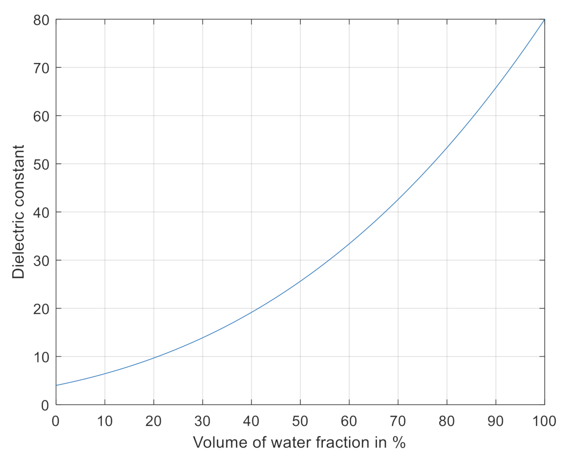
Figure 3.
(a) Cross-section view of the prototype of the proctor mould without a load frame; (b) full assembly view.
Figure 3.
(a) Cross-section view of the prototype of the proctor mould without a load frame; (b) full assembly view.
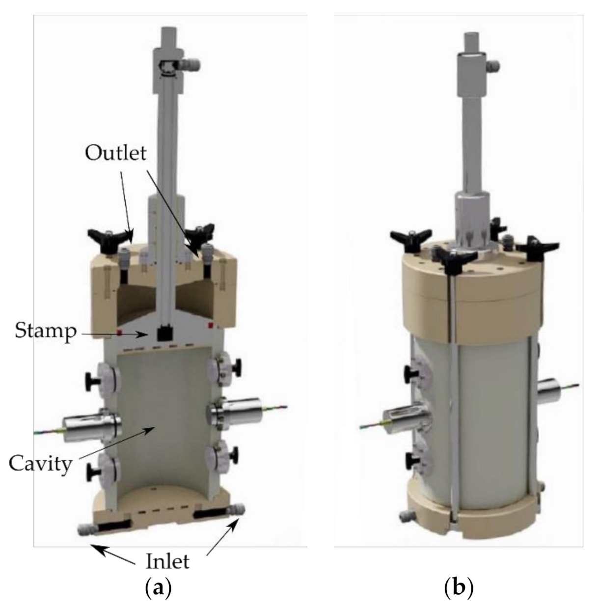
Figure 4.
(a) Geometry of the flat coil; (b) geometry of the interdigital capacitor.
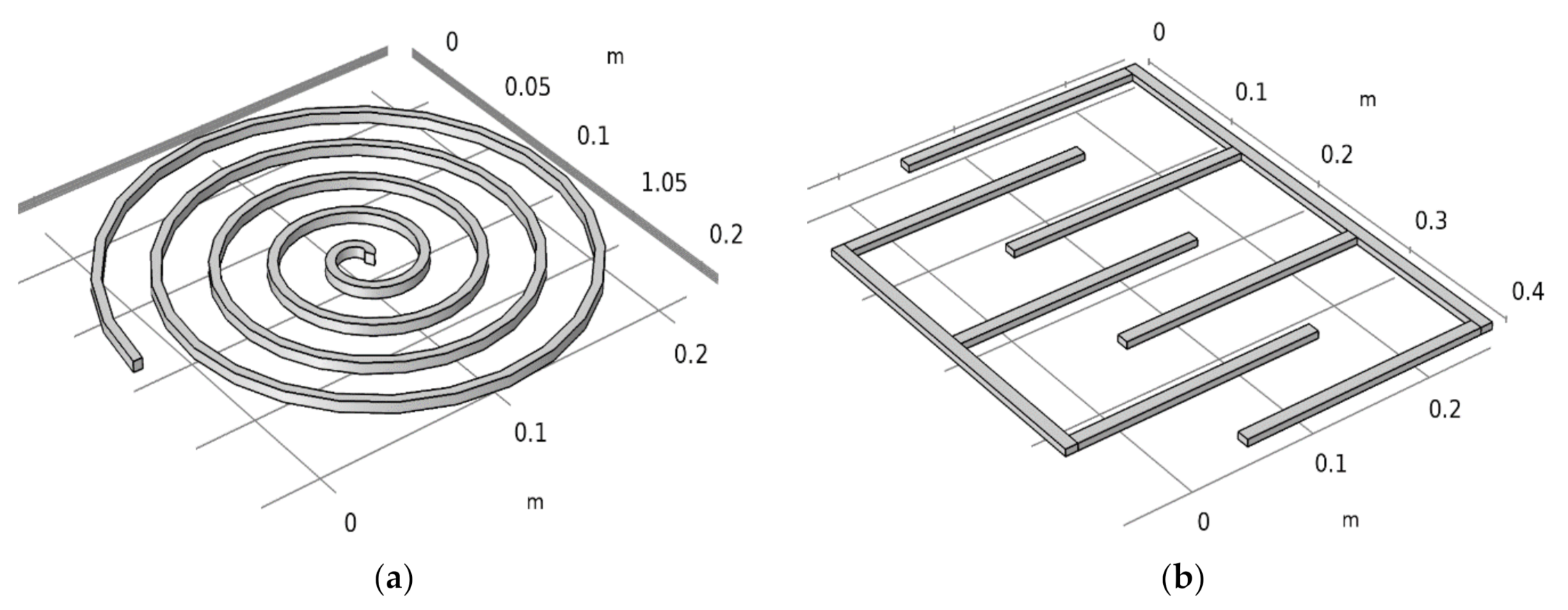
Figure 5.
Simulation results of the absolute value of flat coil impedance as a function of frequency at different volumes of water content.
Figure 5.
Simulation results of the absolute value of flat coil impedance as a function of frequency at different volumes of water content.
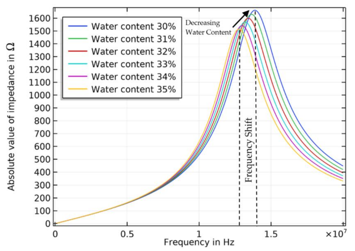
Figure 6.
Simulation results of the absolute value of interdigital capacitor impedance as a function of frequency at different volumes of water content.
Figure 6.
Simulation results of the absolute value of interdigital capacitor impedance as a function of frequency at different volumes of water content.

Figure 7.
Flat coil sensor embedded in the proctor mould.

Figure 8.
Scheme of the functional blocks of the measurement hardware.
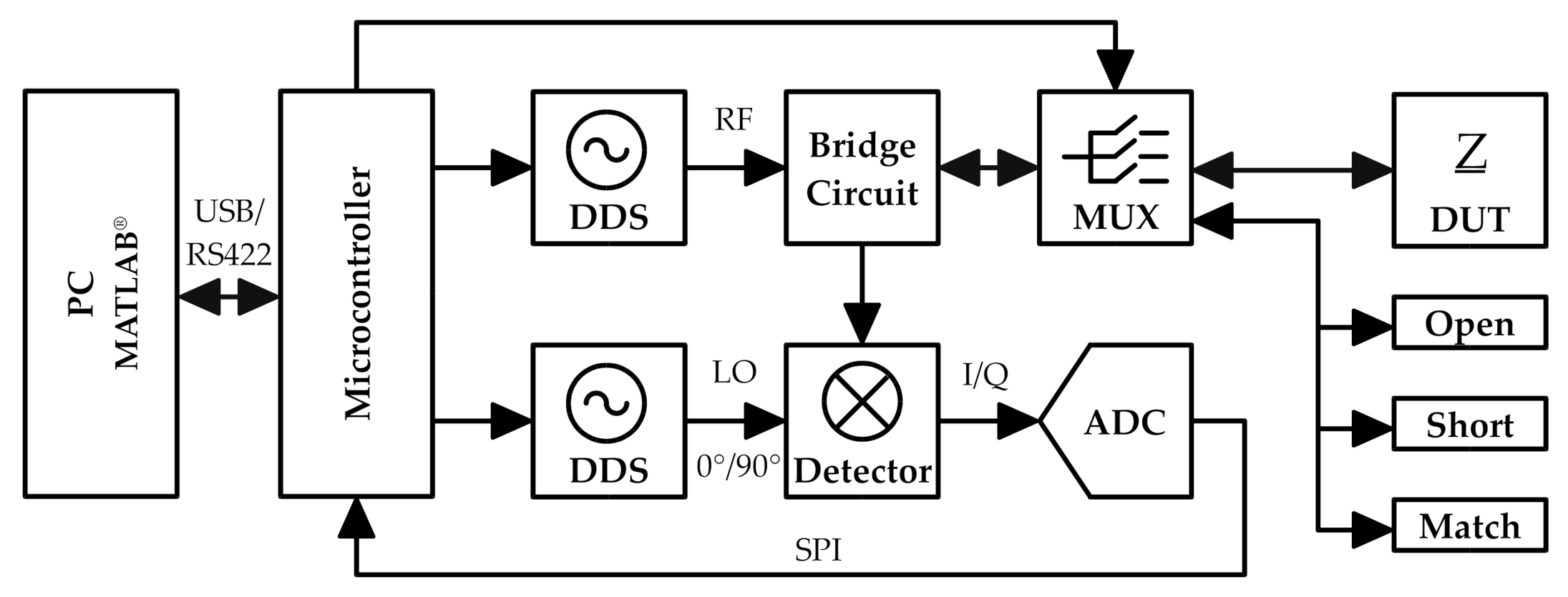
Figure 9.
Wheatstone bridge circuit for complex impedance measurement.
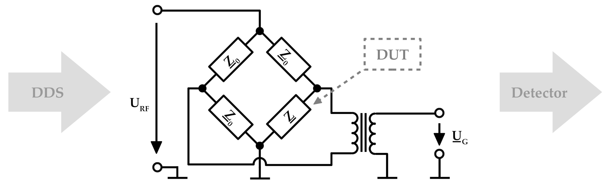
Figure 10.
Impedance spectrum over time during down-top water flow corresponding to the measurements 1–6 (a–f).
Figure 10.
Impedance spectrum over time during down-top water flow corresponding to the measurements 1–6 (a–f).
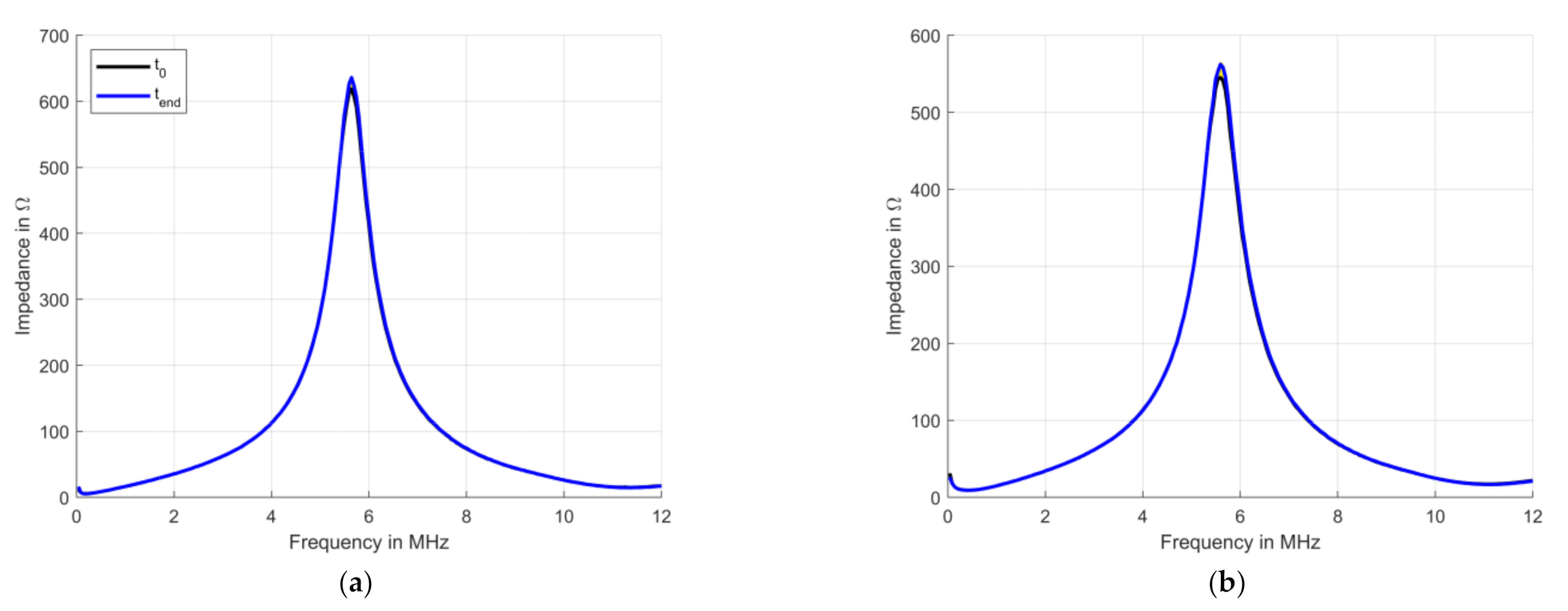
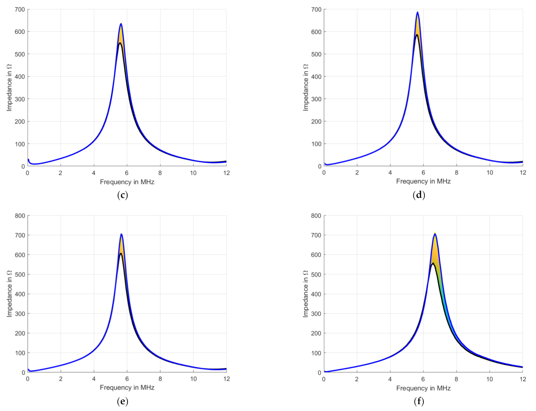
Figure 11.
(a) Impedance over time at resonance frequency of measurement 6. (b) Impedance change over volume change for 39 individual measurements with a fitted curve.
Figure 11.
(a) Impedance over time at resonance frequency of measurement 6. (b) Impedance change over volume change for 39 individual measurements with a fitted curve.

Figure 12.
Equivalent circuit diagram of the measuring arrangement.

Figure 13.
(a) Comparison of the measured spectrum and the modelled system. (b) Percentage difference between the measured spectrum and the modelled system.
Figure 13.
(a) Comparison of the measured spectrum and the modelled system. (b) Percentage difference between the measured spectrum and the modelled system.


Table 1.
Specifications and features of the measurement hardware.
| Frequency Range | to |
| Frequency Resolution | 35 m𝐻𝑧 |
| Impedance Range | |
| Impedance Resolution | |
| Sample Rate | @ 10 Points @ 100 Points per frequency sweep @ 1000 Points |
Table 2.
Input parameters (gravel grain size, hydraulic gradient) and results (volume change, impedance change).
Table 2.
Input parameters (gravel grain size, hydraulic gradient) and results (volume change, impedance change).
| Measurement | Gravel Grain Size [mm] | Hydraulic Gradient | Volume Change [%] | Impedance Change [%] |
|---|---|---|---|---|
| 1 (a) | 2–4 | 7 | 0.26 | 3.65 |
| 2 (b) | 4–8 | 7 | 0.37 | 4.33 |
| 3 (c) | 4–8 | 9 | 1.56 | 17.21 |
| 4 (d) | 4–8 | 11 | 1.68 | 18.17 |
| 5 (e) | 4–8 | 13 | 3.11 | 17.93 |
| 6 (f) | 4–8 | 13 | 5.34 | 29.83 |
Publisher’s Note: MDPI stays neutral with regard to jurisdictional claims in published maps and institutional affiliations. |
© 2021 by the authors. Licensee MDPI, Basel, Switzerland. This article is an open access article distributed under the terms and conditions of the Creative Commons Attribution (CC BY) license (http://creativecommons.org/licenses/by/4.0/).
Share and Cite
MDPI and ACS Style
Clemens, C.; Radschun, M.; Jobst, A.; Himmel, J.; Kanoun, O. Detection of Density Changes in Soils with Impedance Spectroscopy. Appl. Sci. 2021, 11, 1568. https://doi.org/10.3390/app11041568
AMA Style
Clemens C, Radschun M, Jobst A, Himmel J, Kanoun O. Detection of Density Changes in Soils with Impedance Spectroscopy. Applied Sciences. 2021; 11(4):1568. https://doi.org/10.3390/app11041568
Chicago/Turabian StyleClemens, Christoph, Mario Radschun, Annette Jobst, Jörg Himmel, and Olfa Kanoun. 2021. "Detection of Density Changes in Soils with Impedance Spectroscopy" Applied Sciences 11, no. 4: 1568. https://doi.org/10.3390/app11041568
Note that from the first issue of 2016, this journal uses article numbers instead of page numbers. See further details here.