Foreground Objects Detection by U-Net with Multiple Difference Images

Abstract

In video surveillance, robust detection of foreground objects is usually done by subtracting a background model from the current image. Most traditional approaches use a statistical method to model the background image. Recently, deep learning has also been widely used to detect foreground objects in video surveillance. It shows dramatic improvement compared to the traditional approaches. It is trained through supervised learning, which requires training samples with pixel-level assignment. It requires a huge amount of time and is high cost, while traditional algorithms operate unsupervised and do not require training samples. Additionally, deep learning-based algorithms lack generalization power. They operate well on scenes that are similar to the training conditions, but they do not operate well on scenes that deviate from the training conditions. In this paper, we present a new method to detect foreground objects in video surveillance using multiple difference images as the input of convolutional neural networks, which guarantees improved generalization power compared to current deep learning-based methods. First, we adjust U-Net to use multiple difference images as input. Second, we show that training using all scenes in the CDnet 2014 dataset can improve the generalization power. Hyper-parameters such as the number of difference images and the interval between images in difference image computation are chosen by analyzing experimental results. We demonstrate that the proposed algorithm achieves improved performance in scenes that are not used in training compared to state-of-the-art deep learning and traditional unsupervised algorithms. Diverse experiments using various open datasets and real images show the feasibility of the proposed method.

1. Introduction

In video surveillance, the main aim is to detect foreground objects, such as pedestrians, vehicles, animals, and other moving objects. This can be used for object tracking or behavior analysis by further processing. Foreground detection in video surveillance is usually done by comparing a background model image and the current image. Traditional approaches to video surveillance require many steps, including initialization, representation, maintenance of a background model, and foreground detection operation [1,2,3]. Illumination changes, camera jitter, camouflage, ghost object motion, and hard shadows make the robust detection of foreground objects difficult in video surveillance. Many approaches have been proposed to cope with these problems. Since the introduction of deep learning, it has also been adopted in video surveillance. Most algorithms are supervised, while most traditional algorithms are unsupervised. Methods based on deep learning have led to a huge improvement in video surveillance like other domains of image classification, detection, and recognition. However, the use of deep learning in video surveillance has two disadvantages. One is that they have little generalization power. Deep learning achieves improved results compared to the traditional machine learning algorithm, but it still requires improvement in the generalization power. Domain transfer algorithms shows some improvement in this problem. It is well known that, as more training data are used, more accurate results can be obtained through deep learning. The other disadvantage is that deep learning requires a lot of labeled data. In video surveillance, it requires pixel-level labeled data, which are more expensive one than those of image classification and detection. Recently, various datasets that satisfy this requirement have been established with diverse scenarios for video surveillance. In this study, we used the CDnet 2014 dataset [4]. It consists of 53 scenes that cover diverse situations in video surveillance. Typical deep learning algorithms for video surveillance train a new model for each scene using some portion of the data and apply it to the remaining images.

Our goal is to achieve improved generalization power in comparison to recent deep learning-based algorithms in video surveillance. The main contribution of the proposed method is summarized as follows. We present a deep learning-based approach which shows better generalization power than the traditional non-deep learning-based state-of-the-art approach. Deep learning-based approaches achieve better performance than the non-deep learning-based traditional state-of-the-art approach on scenes that are similar to learning environments. However, it requires foreground label images, which require designation per pixel. Therefore, the preparation of training data requires a huge amount of time, while traditional non-deep learning-based algorithms do not require training images. When they are applied to scenes that are different from the training environment without new training on that scene, they show even worse performance than the traditional approach. We present a deep learning-based algorithm that achieves better generalization performance than the traditional non-deep learning-based state-of-the-art approach, and at the same time, it does not require training images. This is possible due to two factors. One is to use multiple difference images as the input of U-Net. The other is to train networks using all training samples from publicly open datasets in visual surveillance. We show the feasibility of the presented method through diverse experimental results.

The rest of the paper is organized as follows. Section 2 gives related works, Section 3 shows the proposed algorithm. The experimental results are shown in Section 4 and, finally, Section 5 gives conclusions.

2. Related Works

Background subtraction and foreground detection in video surveillance have been studied widely. Good surveys of this research are available [5,6,7,8]. We divide them into two groups, namely, approaches that do not use deep learning and those that are based on deep learning.

2.1. Earlier Approaches

Stauffer and Grimson [9] proposed a method called mixture of Gaussian (MOG) that represents the brightness value of each pixel as the combination of Gaussian distributions. They suggested a method to determine the number of the Gaussian mixture and each parameter of the Gaussian distribution using the expectation and maximization algorithm [10]. No special initialization is required because it adapts their parameters as a sequence goes on. Pixels are considered as background when their brightness values belong to the Gaussian mixture model, otherwise, they are considered as foreground. Elgammal et al. [11] proposed a probabilistic non-parametric method using kernel density estimation. Barnich et al. [1] introduced a sample-based method in background modeling. Samples from previous predefined frames are used in background modeling. If there is a predefined group of samples that is close to the current pixel, then it is considered as background, otherwise, it is considered as foreground. Kim et al. [12] proposed a method that uses a codebook. At the initial stage, codewords from intensity, color, and temporal features are constructed. They build up a codebook for later segmentation. The current frame’s pixel values of intensity and color are compared to those of the codewords in the code book. Finally, a foreground or background label is assigned to each pixel by comparing the distance with codewords in the codebook. In the case of a background pixel, the matching codeword is updated. Oliver et al. [13] proposed a method based on principal component analysis, which is called the eigenbackground. The mean and the covariance matrix are computed using a predefined number of images. Here, N eigenvectors are chosen corresponding to the N largest eigenvalues, and they are used as the background model. Incoming images are projected into those eigenvectors, and their distance in those spaces is used to identify the foreground and background.

Wang et al. [14] proposed a method that uses a Gaussian mixture model for the background and uses single Gaussian for the foreground. They employed a flux tensor [15] that can explain variations of optic flow within a local 3D spatio-temporal volume, and it is used in detecting blob motion. With information from blob motion, foreground and background models are integrated to find moving and static foreground objects. Additionally, edge matching [16] is used to classify static foreground objects as ghosts or intermediate motions. Varadarajan et al. [3] proposed a method that applies a region-based mixture of Gaussians for foreground object segmentation to cope with the sensitivity of the dynamic background. Additionally, Chen et al. [17] proposed an algorithm that uses a mixture of Gaussians in a local region. At each pixel level, the foreground and background are modeled using a mixture of Gaussians. Each pixel is determined to be foreground or background by finding the highest probability of the center pixel around an N × N region.

Sajid and Cheung [18] proposed an algorithm to cope with sudden illumination changes by using multiple background models through single Gaussians and different color representations. K-means clustering is used to classify the pixels of input images. For each pixel, K models are compared, and the group that shows the highest normalized cross-correlation is chosen. An RGB and YCbCr color frame is used, and segmentation is done for each color, which yields six segmentation masks. Finally, background segmentation is performed by integrating all available segmentation masks.

Hofmann et al. [19] proposed an algorithm that improves Barnich et al. [1]. They replace the global threshold R with an adaptive threshold R(x) that depends on the pixel location and a metric of the background model which is called background dynamics. The threshold R(x) and the model update rate are determined by a feedback loop using the additional information from the background dynamics. They showed that it can cope with a dynamic background and highly structured scenes. Tiefenbacher et al. [20] proposed an algorithm that improves the algorithm introduced by Hofmann et al. [19] by controlling the updates of the pixel-wise thresholds using a PID controller. St-Charles et al. [2] also proposed an improved algorithm by using local binary similarity patterns [21] as additional features of pixel intensities and slight modification of the update mechanism of the thresholds and the background model.

2.2. Deep Learning-Based Approaches

Braham and Droogenbroeck [20] proposed the first scene-specific convolutional neural network (CNN)-based algorithm for background subtraction. A fixed background model is generated by a temporal median operation over the first 150 video frames. Then, image patches centered on each pixel are extracted from both the current and background images. The combined patches are used as the input of the trained CNN, and it outputs the probability of foreground. They evaluated their algorithm on the 2014 ChangeDetection.net dataset (CDnet 2014) [22]. The CNN requires training for each sequence in CDnet 2014. It requires a long computation time because patches from each pixel are required to pass the CNN, and it is similar to the sliding window approach in object detection. Babaee et al. [23] proposed a method that uses a CNN to perform the segmentation of foreground objects, and they use a background model that is generated using the SuBSENSE [2] and Flux Tensor [14] algorithms. Spatial median filtering is used for the post-processing of the network outputs. Wang et al. [24] proposed multi-scale convolutional neural networks with cascade structure for background subtraction. Additionally, they trained a network for each video in the CDnet 2014 dataset. More recently, Lim et al. [25] proposed an encoder–decoder-type neural network for foreground segmentation called FgSegNet. It uses a pretrained convolutional network of VGG-16 [26] as the encoding part with a triplet network structure. In the decoding part, a transposed convolutional network is used. Their network is trained by randomly selecting some training samples for each video in CDnet 2014.

Zeng et al. [27] proposed a multi-scale fully convolutional network architecture that takes advantage of various layer features for background subtraction. Zheng et al. [28] proposed an algorithm that combines traditional background subtraction and semantic segmentation [29]. The output of semantic segmentation is used to update the background model through feedback. Their result shows that it achieves the best performance among unsupervised algorithms in CDnet 2014. Sakkos et al. [30] presented a robust model that consists of a triple multi-task generative adversarial network (GAN) that can detect foreground even in exceptionally dark or bright scenes and in continuously varying illumination. They generate low- and high-brightness image pairs using the gamma function from a single image and use them in training by simultaneously minimizing GAN loss and segmentation loss. Patil et al. [31] proposed a motion saliency foreground network (MSFgNet) to estimate the background and to find the foreground in video frames. Original video frames are divided into a number of small video streams, and the background is estimated for each divided video stream. The saliency map is computed using the current video frame and the estimated background. Finally, an encoder–decoder network is used to extract the foreground from the estimated saliency maps. Varghese et al. [32] investigated visual change, aiming to accurately identify variations between a reference image and a new test image. They proposed a parallel deep convolutional neural network for localizing and identifying the changes between image pairs.

Akilan et al. [33] proposed a 3D convolutional neural network with long short-term memory (LSTM) to include temporal information in a deep learning framework for background subtraction. This is similar to our approach in terms of using temporal information. We use multiple difference images as the input of networks, while they extracted temporal information by LSTM. Yang et al. [34] proposed a method to apply multiple images to fully convolutional networks (FCNs). When selecting multiple input images, images close to the current are selected more. The studies in [33,34] belong to the method of using multiple input images in the same way as the proposed method. In the case of [33,34], multiple original images are used, whereas the proposed method is different in using multiple difference images.

3. Proposed Method

Unlike general object segmentation, proper acquisition of temporal information as well as spatial information is essential for robust foreground object detection in video surveillance. If we rely only on spatial information in the foreground object detection process, it may be difficult to determine whether the vehicle is moving or not. However, this problem can be solved if temporal information from past images is used.

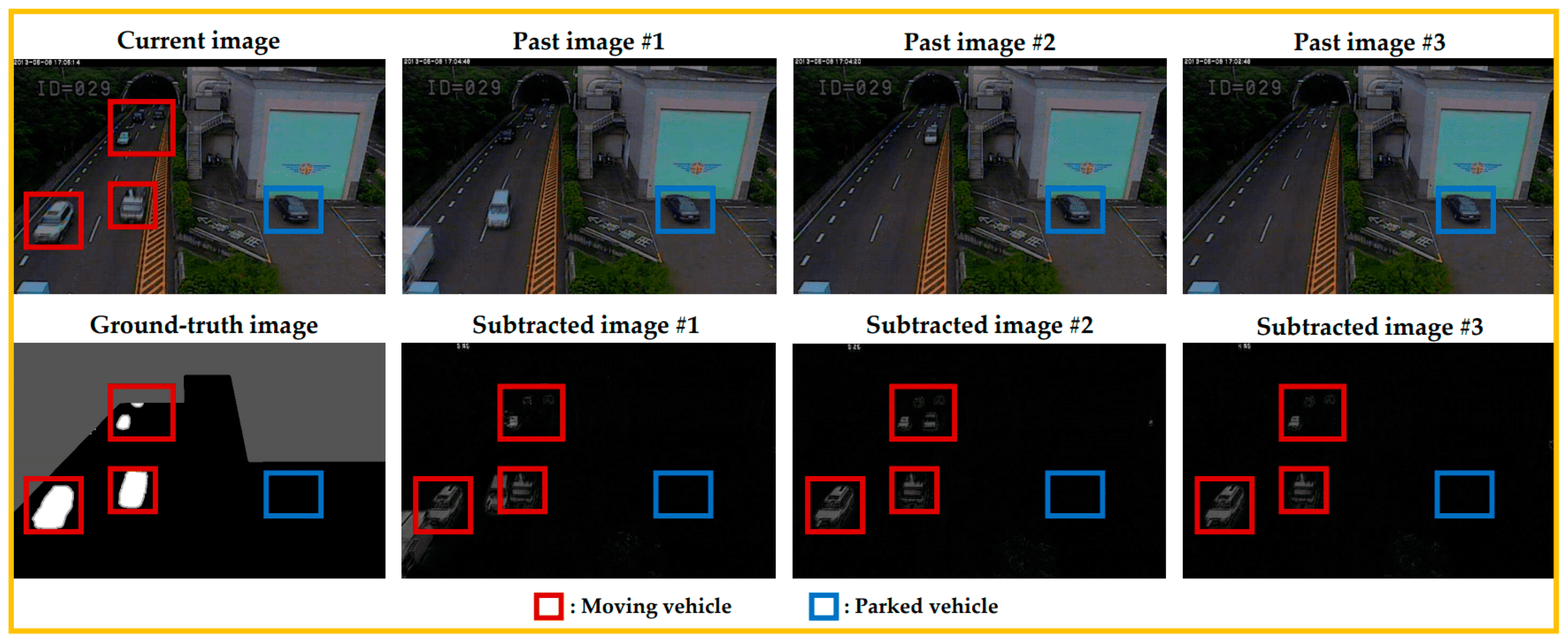
Figure 1 shows the difference images between the current image and a number of past images. Using only spatial information existing in the current image has a limitation in distinguishing between the driving vehicle in the red box in Figure 1 and the parked vehicle in the blue box. On the other hand, when the difference image is used as input data for a deep learning model, it is possible to distinguish between a moving object and a stationary object. However, as can be seen from the difference images in Figure 1, there is a problem in that both the location where the foreground object existed in the past and the location that existed in the present view are displayed in the difference image between the current image and the past image. In addition, elements such as snow and rain and dynamic background objects such as moving bushes in bad weather conditions show high difference values even though they are background objects. In order to solve these problems, the proposed method uses many difference images, not a single difference image, as input data.

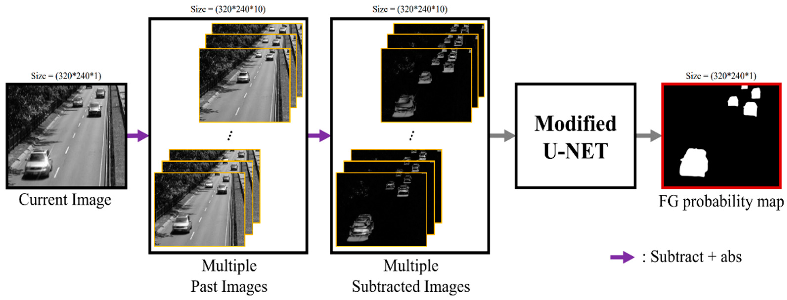
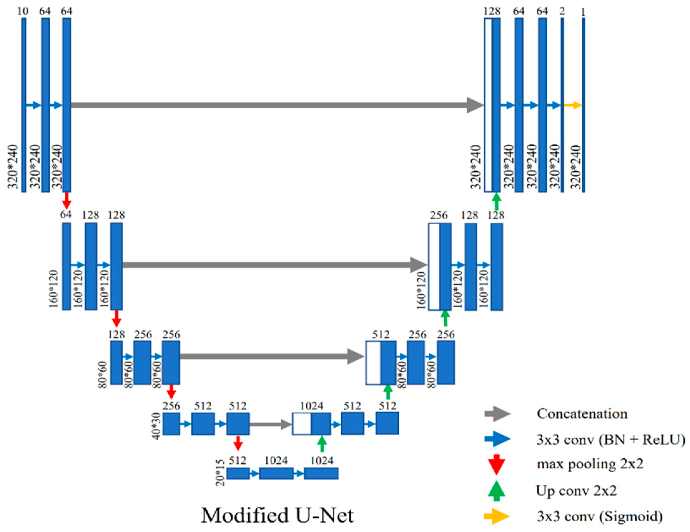
We adopt U-Net [35], which uses a gray or color image as the input of the network. We adjust it to use multiple difference images. Figure 2 shows the overall structure of the proposed algorithm. A network structure that uses multiple difference images as the input of U-Net [35] is shown in Figure 3. Difference images are obtained by subtracting each past image from the current image. The total number of difference images and the frame interval in subtraction are the hyper-parameters. We choose them through the analysis of experimental results. We choose 10 difference images as the number of inputs of the network through experiments. The size of the input is changed to 320(W) × 240(H) × 10(C), while the original U-Net uses input images of 572(W) × 572(H) × 1(C). U-Net [35] does not use padding in the convolutional layer and uses “copy and crop” in the layer connection process, so it outputs an image of 388x388 in size, which is different from the input image size of 572 × 572. In visual surveillance, all areas of the image need to be classified into foreground or background. Therefore, we prevented the size reduction of the output according to the convolutional layer by using padding in all layers of U-Net, and layers were connected using concatenation without cropping to make the size of the input image and the output image the same. The size of the input image was 320 × 240, which is an image size mainly used in the visual surveillance.

Batch normalization is used between each convolutional layer and the nonlinear function. Here, 2 × 2 max polling is used and the filter size of all convolution layers is 3 × 3. A rectified linear unit (ReLU) is used as the activation function in all layers except the last layer where a sigmoid function is used. We use the sigmoid function on the final layer to make the foreground and background map have a value between 0 and 1. The output of the final convolution layer gives the segmentation map by the sigmoid function. Finally, a segmentation map of 320(W) × 240(H) × 1(C) is obtained. The total number of parameters of the proposed structure is 31,064,261, and the number of learnable parameters is 31,050,565.

Binary cross-entropy is used as the loss, which is defined as

$$\mathrm{L}=\frac{1}{N}{\displaystyle \sum }_{i=0}^N-\left(y_{i}log{\widehat{y}}_i+(1-y_i\right)\log (1-{\widehat{y}}_i))$$

(1)

where $y_i$ is the ground truth label of the i-th pixel is, ${\widehat{y}}_i$ is the label estimated by networks, and $\mathrm{N}$ is the total number of pixels in the image. We train the proposed structure using the CDnet 2014 dataset, and 24 scenes are selected from the total of 53 scenes. We select 200 images for each scene and randomly divide them into 160 training images and 40 validation images. When 24 scenes consisting of 4800 images are used in the training, 3840 images and 960 images are used for the training and validation, respectively.

The Keras framework [36] with TensorFlow as a backend is used in implementation. The initial values of parameters in the networks are initialized using the He normal initializer [37]. We do not use the pretrained weights of VGG-16 [26] for our model because we use multiple difference images as the input, while VGG deals with raw input images. We train our network using the Adam optimizer [38] with an initial learning rate as 0.001, ${\beta }_1$ as 0.9, ${\beta }_2$ as 0.999, and $\mathsf{\epsilon }$ as ${10}^{-8}$. If the validation loss does not decrease in five successive epochs, the learning rate is reduced by half. The learning process is stopped if the validation loss does not decrease in 10 successive epochs within the maximum of 100 epochs. The CDnet 2014 dataset provides four labels of static, hard shadow, outside region of interest, and unknown motion as the ground truth of the segmentation map. Preprocessing is performed to divide the pixel value of the ground truth images by 255. We set static as 0 and motion as 1 in the computation of loss. The outside region of interest area and the unknown motion are not used in the computation of loss.

4. Experimental Results

In the experiment, the proposed algorithm is compared with the traditional algorithms of SuBSENSE [2], CwisarD [39], Spectral360 [40], GMM [9], and PAWCS [41] and deep learning-based algorithms of FgSegNet-v2 [42] and modified FgSegNet-v2. The original FgSegNet-v2 [42] algorithm uses one RGB image as the input of a network. We modify it to use multiple difference images as the input of a network, like the proposed algorithm, and we denote it as modified FgSegNet-v2. Data for training consisted of a training set and validation set, and the performance of each algorithm was evaluated using a test set that was not used for training.

The following experiment was performed to show the performance of the proposed algorithm.

(1) Comparison when using multiple original images and multiple difference images as the input of a network; we show the superiority of the proposed algorithm through this.

(2) Comparison between learning using data obtained in one environment and learning using all data obtained in various environments; we show that the proposed algorithm gives improved results in unknown scenes.

Experiments were done using the CDnet 2014 dataset [4]. They consisted of 53 scenes from 11 categories, as shown in

Table 1. List of scenes in the CDnet 2014 dataset (bold indicates the scene used in training).

Categories (Total Number of Scenes/Number of Scenes Used for Training)	Scene Names
Baseline (4/2)	Highway, Office, Pedestrians, PETS2006
Camera Jitter (4/2)	Badminton, Sidewalk, Traffic, Boulevard
Bad Weather (4/2)	Skating, Wet snow, Blizzard, Snowfall
Dynamic Background (6/3)	Boats, Canoe, Fountain1, Fountain2, Fall, Overpass
Intermittent Object Motion (6/2)	Abandoned box, Street light, Parking, Sofa, Tram stop, Winter drive way
Low Framerate (4/2)	Port_0_17 fps, Tram crossroad_1 fps, Tunnel exit_0_35fps, Turnpike_0_5fps
Night Videos (6/3)	Bridge entry, busy boulevard, fluid highway, Street corner at night, Tram station, Winter street
PTZ (4/0)	Continuous pan, Intermittent pan, Two position ptz cam, Zoom in zoom out
Shadow (6/3)	Back door, Copy machine, Bungalows, Bus station, Cubicle, People in shade
Thermal (5/3)	Corridor, Library, Lakeside, Dining room, Park
Turbulence (4/2)	Turbulence0, Turbulence1, Turbulence2, Turbulence3

, and they dealt with diverse situations that could occur during visual surveillance. We evaluated the foreground object detection algorithms using a variety of metrics that are widely used in visual surveillance, namely, recall, precision, F-measure (FM), percentage of wrong classification (PWC), false positive rate (FPR), false negative rate (FNR), and specificity (SP):

$$\mathrm{Precision}=\frac{TP}{TP+FP}$$

$$\mathrm{Recall}=\frac{TP}{TP+FN}$$

$$\mathrm{FM}=2\times \frac{Precision\times Recall}{Precision+Recall}$$

$$\mathrm{PWC}=\frac{FP+FN}{TP+TN+FP+FN}$$

$$\mathrm{FPR}=\frac{FP}{FP+TN}$$

$$\mathrm{FNR}=\frac{FN}{TP+FN}$$

$$\mathrm{SP}=\frac{TN}{TN+FP}$$

where TP, TN, FP, and FN mean true positive, true negative, false positive, and false negative, respectively.

In Table 1, bold letters represent the 24 scenes used in the training. We used 200 images for each scene in training. Test statistics are obtained by using scenes not used in the training in Table 1. Ten difference images under a five-frame interval were used as the input of networks. Subtracting by mean was used for the preprocessing of the input data. In both cases, four scenes of the pan–tilt–zoom (PTZ) category were not used in the training. The proposed method has a weakness for the category of PTZ where images are obtained through panning of the camera. In video surveillance, cameras are usually fixed at a predefined location. Scenes in the PTZ category are not common situations in video surveillance. Therefore, experiments are done using 49 scenes from 10 categories, excluding the PTZ category. Computation was done using one Intel i7-7820X CPU and an NVIDIA RTX 2080Ti GPU. The computation time for each input was 30 ms, which was obtained by averaging the processing time of 100 trials. In the case of FgSegNet-v2 [42], a deep learning-based method, it took 9 ms to process one image in the same PC environment. This is a faster processing speed than the proposed method, but the proposed method shows much better generalization ability in the real environment. Additionally, the proposed method can be computed over 30 fps. Therefore, it was judged that the proposed method has an appropriate level of model size and computational cost to use in a real environment.

First, we present the experimental results of training using only one scene in the CDnet 2014 dataset. After training using one scene, we applied it to other scenes to assess the generalization ability.

Table 2. Comparison of results obtained by training using one scene (Highway) in the CDnet 2014 dataset.

	Highway Scene		All Scenes		Scenes Not Used in Training
	FM	PWC	FM	PWC	FM	PWC
Proposed	0.99	0.08	0.47	3.61	0.46	3.68
FgSegNet-v2 [42]	1.00	0.02	0.25	11.1	0.23	11.4

shows a comparison of the proposed method and FgSegNet-v2 [42], which produces state-of-the-art results on the CDnet 2014 dataset. FgSegNet-v2 was used to train a separate network for each scene in the CDnet 2014 dataset, and test statistics were obtained for each scene. The proposed method and FgSegNet-v2 were trained using only a highway scene in the CDnet 2014 dataset. FgSegNet-v2 uses one RGB image as input, while the proposed algorithm uses 10 difference images as input. FgSegNet-v2 achieved a better result than the proposed algorithm in a scene that was used in the training. Though the proposed method showed dramatic improvement in comparison to FgSegNet-v2 for other scenes that were not used in the training, the overall performance of the proposed method still requires improvement because it achieves much lower performance than SuBSENSE [2]. We can conclude that training using only a highway scene does not guarantee generalization power for other scenes. Therefore, we trained the proposed algorithm using all the scenes except the PTZ category in the CDnet 2014 dataset to improve the generalization ability.

Table 3. Results of proposed method which is trained using 24 scenes in CDnet 2014 dataset.

Categories	FM	PWC	Recall	Precision	FPR	FNR	SP
Baseline	0.9535	0.1301	0.9481	0.9597	0.0006	0.0519	0.9994
Camera Jitter	0.7759	3.5410	0.7563	0.8461	0.0084	0.2437	0.9916
Bad Weather	0.9266	0.1741	0.9628	0.9007	0.0012	0.0372	0.9988
Dynamic BG	0.8952	0.2805	0.8892	0.9033	0.0012	0.1108	0.9988
Int. Obj. Motion	0.7509	3.0798	0.9169	0.6792	0.0306	0.0831	0.9694
Low Framerate	0.7854	0.9016	0.9256	0.7204	0.0088	0.0744	0.9912
Night Videos	0.8553	0.5602	0.8717	0.8437	0.0035	0.1283	0.9965
Shadow	0.9108	0.6420	0.9251	0.9037	0.0042	0.0749	0.9958
Thermal	0.9319	0.6305	0.9688	0.9006	0.0059	0.0312	0.9941
Turbulence	0.8536	0.2404	0.9766	0.7881	0.0023	0.0235	0.9977
Average	0.8635	1.0301	0.9130	0.8437	0.0072	0.0870	0.9928
Scenes used in training	0.9649	0.1580	0.9788	0.9529	0.0013	0.0212	0.9987
Scenes not used in training	0.7662	1.8674	0.8499	0.7389	0.0128	0.1501	0.9872

and

Table 4. Comparison result of FM score by proposed method and other methods on the CDnet 2014 dataset.

Scenes	Proposed	Modified FgSegNet-v2	FgSegNet-v2 [42]	SuBSENSE [2]	CwisarD [39]	Spectral-360 [40]	GMM [9]
Baseline	0.954	0.940	0.814	0.950	0.908	0.933	0.825
Camera Jitter	0.776	0.769	0.613	0.815	0.781	0.716	0.597
Bad Weather	0.927	0.919	0.876	0.862	0.684	0.757	0.738
Dynamic Background	0.895	0.883	0.619	0.818	0.809	0.787	0.633
Int. Obj. Motion	0.751	0.719	0.584	0.657	0.567	0.566	0.633
Low Framerate	0.785	0.750	0.742	0.645	0.641	0.644	0.537
Night Videos	0.855	0.831	0.703	0.560	0.374	0.483	0.410
Shadow	0.911	0.893	0.734	0.899	0.841	0.884	0.737
Thermal	0.932	0.929	0.799	0.817	0.762	0.776	0.662
Turbulence	0.854	0.896	0.521	0.779	0.723	0.543	0.466
Average	0.864	0.850	0.697	0.777	0.706	0.706	0.619

show the result of the proposed algorithm, which was trained using 24 scenes in CDnet 2014 dataset. The proposed method shows superior performance compared to other algorithms, with FM scores of 0.927 and 0.895, respectively, even in “Bad Weather” and “Dynamic Background” categories, where a large amount of noise is included in the difference image.

Table 4 shows a comparison of the results obtained by the proposed algorithm and other algorithms. The proposed method, FgSegNet-v2 [42], and modified FgSegNet-v2 were trained using the same 24 scenes in the CDnet 2014 dataset. The proposed method, FgSegNet-v2, and modified FgSegNet-v2 are deep learning-based algorithms that require training samples. SuBSENSE [2], CwisarD [39], Spectral-360 [40], and GMM [9] are traditional algorithms that do not require training samples, and their experimental statistics shown in Table 4 are those reported in the literature. The proposed algorithm achieved the best performance, except for camera jitter and turbulence categories in the CDnet 2014 dataset. Training the original FgSegNet-v2 using 24 scenes in the CDnet 2014 dataset produced an even worse performance than the traditional SuBSENSE algorithm [2]. Simply training using multiple scenes without changing the network cannot guarantee generalization power. The proposed algorithm, which uses multiple difference images as input, achieves a meaningful improvement. We can conclude that the proposed algorithm provides greater generalization ability than other algorithms.

The original FgSegNet-v2 has no generalization ability in other scenes that are not used in training. Modifying its input to be multiple difference images, like in the proposed method, leads to dramatic improvement. Therefore, we can conclude that using multiple difference images as the input of the network could increase its generalization ability.

4.1. Multiple Difference Images vs. Multiple Original Images

In this section, we show experimental results according to the types of input images. We compare two cases of using multiple original images and multiple difference images as the input of networks. FgSegNet-v2 [42] predicts foreground objects using only the current image as the input of the networks. We modify it to use multiple original images or multiple difference images. In both cases, subtracting with mean is used as preprocessing. Training is done using 24 scenes in Table 1. Two hundred images from each scene are used, so 4800 images in total are used in training.

Table 5. Comparison results of using multiple original images and multiple difference images as the input of networks within a 50-frame range.

Number of Original or Difference Images	Overall		Scenes Used for Training		Scenes Not Used for Training
	FM	PWC	FM	PWC	FM	PWC
6 (org)	0.84	1.43	0.96	0.12	0.72	2.69
5 (diff)	0.86	1.06	0.97	0.13	0.76	1.95
11 (org)	0.84	1.36	0.98	0.06	0.71	2.62
10 (diff)	0.86	1.03	0.96	0.16	0.77	1.87

shows the performance of the trained network on CDnet 2014 dataset according to the input of original images and multiple difference images. The numbers of original images and difference images are varied according to the interval between frames, as shown in Table 5, where 50 frames are considered for the input of the network. We show performance in two different aspects. One is applying a trained network on scenes used in training. The other is applying a trained network on scenes that are not used in the training. Using multiple original images gives a slightly better result than using multiple difference images in scenes used in training. However, using multiple difference images shows a distinctly better performance than for scenes which are not used in the training. At 10-frame intervals, we could reach a 27.5% reduction in false detection by using five difference images compared to using six original images, and we could reach a 28.6% reduction in false detection by using 10 difference images compared to using 11 original images. We can conclude that using multiple difference images as the input of networks gives improved accuracy and generalization power.

4.2. Frame Intervals in Multiple Difference Images

We show the experimental results by varying the number of difference images and the interval between frames in difference image computation. Training is done using 24 scenes in Table 1. Two hundred images are used for each scene, so 4800 images in total are used in training.

Table 6. A comparison result by changing the number of difference images under a five-frame interval.

Number of Difference Images	All Scenes		Scenes Used for Training		Scenes Not Used for Training
	FM	PWC	FM	PWC	FM	PWC
5	0.84	1.10	0.95	0.30	0.74	1.86
10	0.86	1.03	0.96	0.16	0.77	1.87
15	0.85	1.06	0.96	0.26	0.75	1.84
20	0.84	1.09	0.93	0.30	0.75	1.86

shows the experimental results by varying the number of difference images at the fixed interval of five frames.

Table 7. A comparison result by changing frame intervals to within 50 frames.

Number of Difference Images	All Scenes		Scenes Used for Training		Scenes Not Used for Training
	FM	PWC	FM	PWC	FM	PWC
2	0.85	1.24	0.96	0.18	0.75	2.26
5	0.86	1.06	0.97	0.13	0.76	1.95
10	0.86	1.03	0.96	0.16	0.77	1.87
50	0.84	1.22	0.96	0.18	0.72	2.21

shows the experimental results by varying intervals between frames in computing difference images at the fixed range of 50 frames. Evaluation is done using CDnet 2014 datasets except the PTZ category. Three experimental statistics of performance using all scenes, scenes used for training, and scenes not used for training are presented in Table 6 and Table 7. The number of difference images and the frame interval between successive images are closely related to the speed of moving foreground objects. We think that there are different optimal numbers of difference images and intervals according to the speed of moving foreground objects. Small differences in performance appear according to the variation of the number of difference images and frame intervals in the Cdnet 2014 dataset. Finally, we set the number of difference images as 10 and the interval between frames as five based on these experimental results which show better performance in scenes not used in training.

4.3. Generalization Ability Test Using Scenes Not Used in Training

Having a good generalization power is one of the main goals of machine learning. Though deep learning has shown a big jump in performance in various areas, it still requires an improvement in the generalization power. We show the improved generalization power of the proposed method by applying it on the scenes that are not used in the training. The proposed algorithm is compared to three algorithms, SuBSENSE [2], modified FgSegNet-v2, and FgSegNet-v2 [42]. We adjust FgSegNet-v2 to use multiple difference images as input, like the proposed method, and we denote it as modified FgSegNet-v2. Experiments were done by training the proposed method, modified FgSegNet-v2, and FgSegNet-v2 using the same 24 scenes in the CDnet 2014 dataset, which are shown in Table 1.

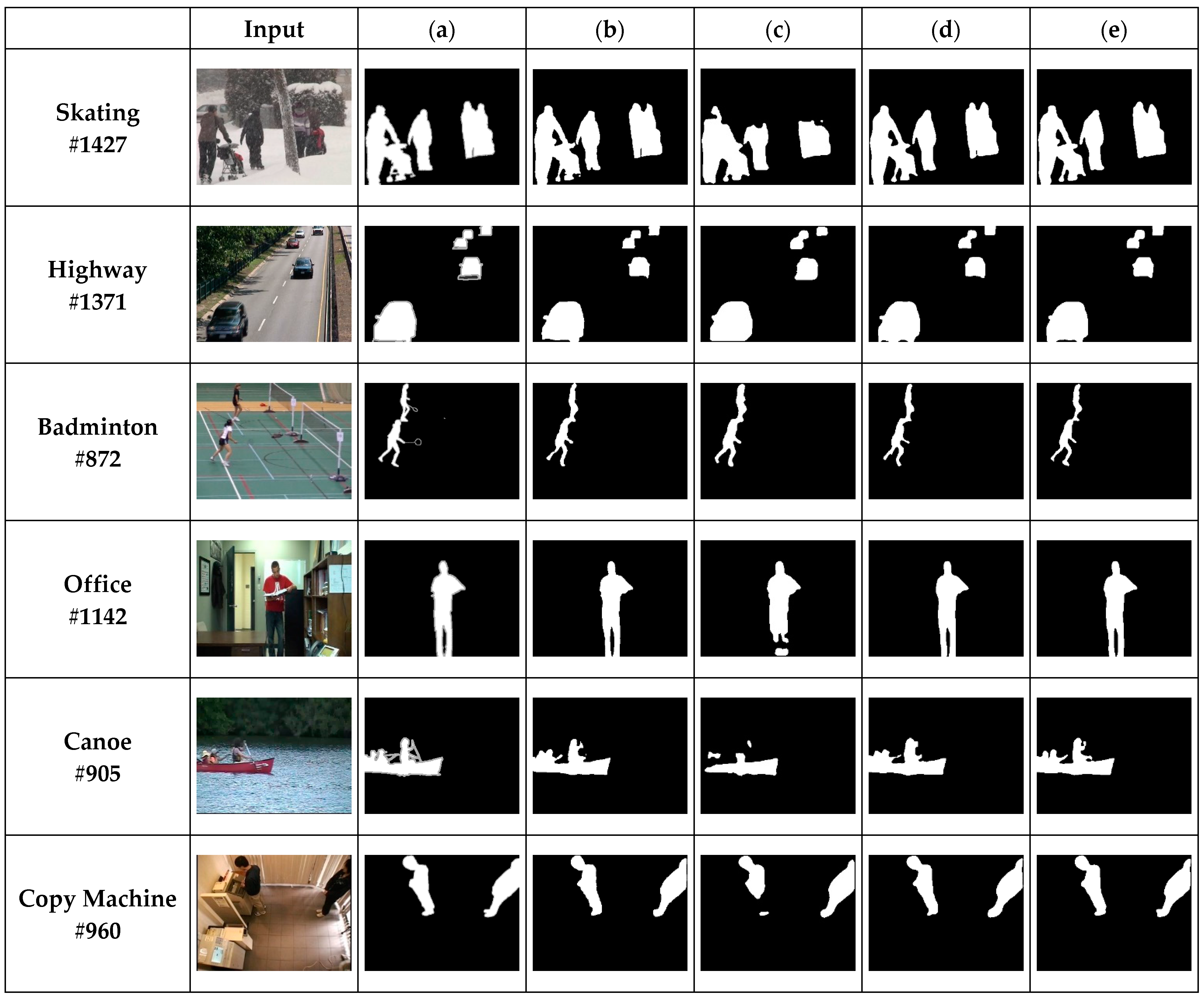
First, we evaluate the generalization power on the CDnet 2014 dataset. We investigated the generalization ability by applying the trained networks to the other 29 scenes that were not used in training in the CDnet 2014 dataset. Second, we present the results obtained by applying the trained networks to scenes in the SBI2015 dataset [43] and scenes that we acquired ourselves. The SBI2015 dataset and scenes that we acquired were not used in training. Figure 4 shows the results obtained on scenes used for training in the CDnet 2014 dataset. Figure 4a shows the original image and the corresponding frame number of the scene. Figure 4b shows the ground truth segmentation map. The results of SuBSENSE [2], the proposed method, modified FgSegNet-v2, and FgSegNet-v2 [42] are presented in Figure 4b–e. The deep learning-based methods of the proposed method, modified FgSegNet-v2, and FgSegNet-v2 give better results than the traditional approach of SuBSENSE [2]. Through this, we can ascertain that deep learning-based algorithms give superior results compared to traditional a BGS algorithm in scenes used in the training.

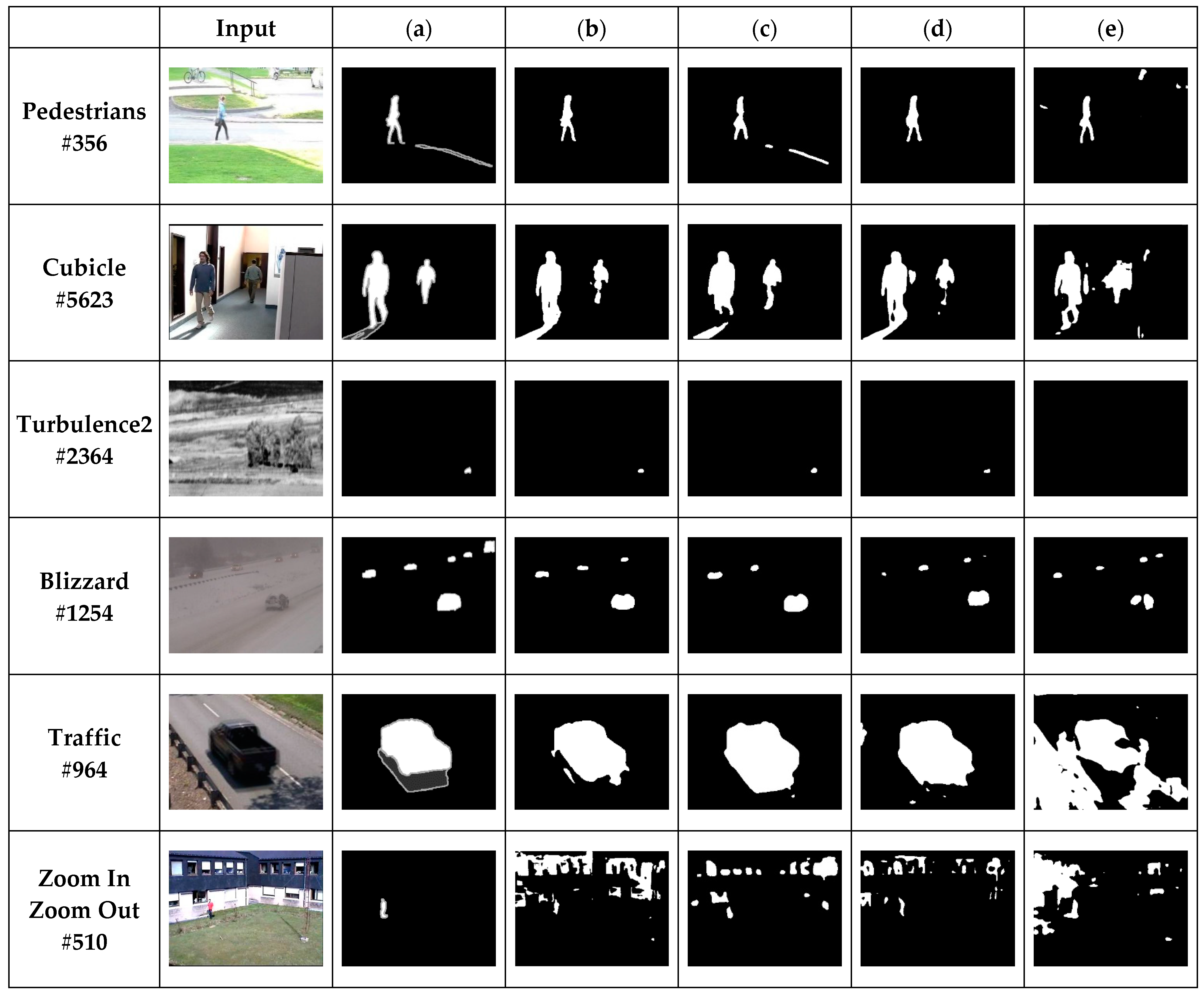
Figure 5 shows the results obtained on scenes that were not used for training in the CDnet 2014 dataset. We can notice a clearly different tendency in Figure 4. FgSegNet-v2 [42] produces the worst results among the four algorithms. It produces even worse results than the non-deep learning-based method of SuBSENSE [2]. We can conclude that the original FgSegNet-v2 is efficient in scenes that were used for training, and it has little generalization ability. This can also be noticed quantitatively in Table 4. The proposed method and modified FgSegNet-v2 achieve better results than SuBSENSE even in scenes not used in training. Through this, it can be confirmed that the generalization ability is improved considerably by simply changing the input structure without changing the structure of the deep learning model.

We present quantitative results obtained using the SBI2015 dataset [43] to show the generalization ability of proposed method. SBI2015 provides 14 scenes in total. We do not use the Toscana scene because it consists of six images that are not continuous. In addition, “Snellen” and “Foliage” scenes treated moving leaves as foreground labels. This classification differs from the foreground concept used in video surveillance. Moving leaves are generally classified as dynamic background, and we think that they should be treated as background labels. Therefore, in experiments, “Snellen” and “Foliage” scenes were also excluded from the evaluation. The proposed method, FgSegNet-v2 [42], PAWCS [41], and the SuBSENSE [2] algorithm were compared, and the results are shown in

Table 8. Comparison of FM score by the proposed method and other algorithms on the SBI2015 dataset.

Scene	Ours	Modified FgSegNet-v2	PAWCS [41]	SuBSENSE [2]	FgSegNet-v2 [42]
Board	0.8114	0.8086	0.7798	0.5777	0.5816
CAVIAR1	0.9566	0.9342	0.8589	0.9144	0.9115
CAVIAR2	0.8094	0.8192	0.6772	0.8714	0.0306
CaVignal	0.8634	0.9102	0.3697	0.3980	0.7704
Candela	0.6402	0.6646	0.8725	0.5356	0.4144
Hall&Monitor	0.9384	0.8878	0.7411	0.7758	0.7365
Highway1	0.8465	0.8619	0.7015	0.5523	0.4263
Highway2	0.9559	0.9537	0.9031	0.8937	0.2277
HumanBody2	0.9415	0.9342	0.7013	0.8346	0.5978
IBMtest2	0.9574	0.9548	0.9386	0.9390	0.4197
People&Foliage	0.4474	0.3033	0.3162	0.2660	0.4930
Mean	0.8335	0.8211	0.7145	0.6871	0.5100

. The proposed method achieved a better performance than other algorithms. The proposed method shows low FM scores in the “Candela” and “People&oliage” scenes. Since the proposed method receives images in a range of 50 frames, it shows insufficient performance in the “Candela” scene where there is a foreground object that has been stopped for a long time. Additionally, in the “People&Foliage” scene, both moving people and bushes are classified as foreground objects. In visual surveillance, moving bushes should be classified as dynamic background, but in the scene they are classified as foreground, so most methods, including the proposed method, show very low performance. Furthermore, FgSegNet-v2 achieved much lower performance than the PAWCS and SuBSENSE algorithms, as seen in Figure 5.

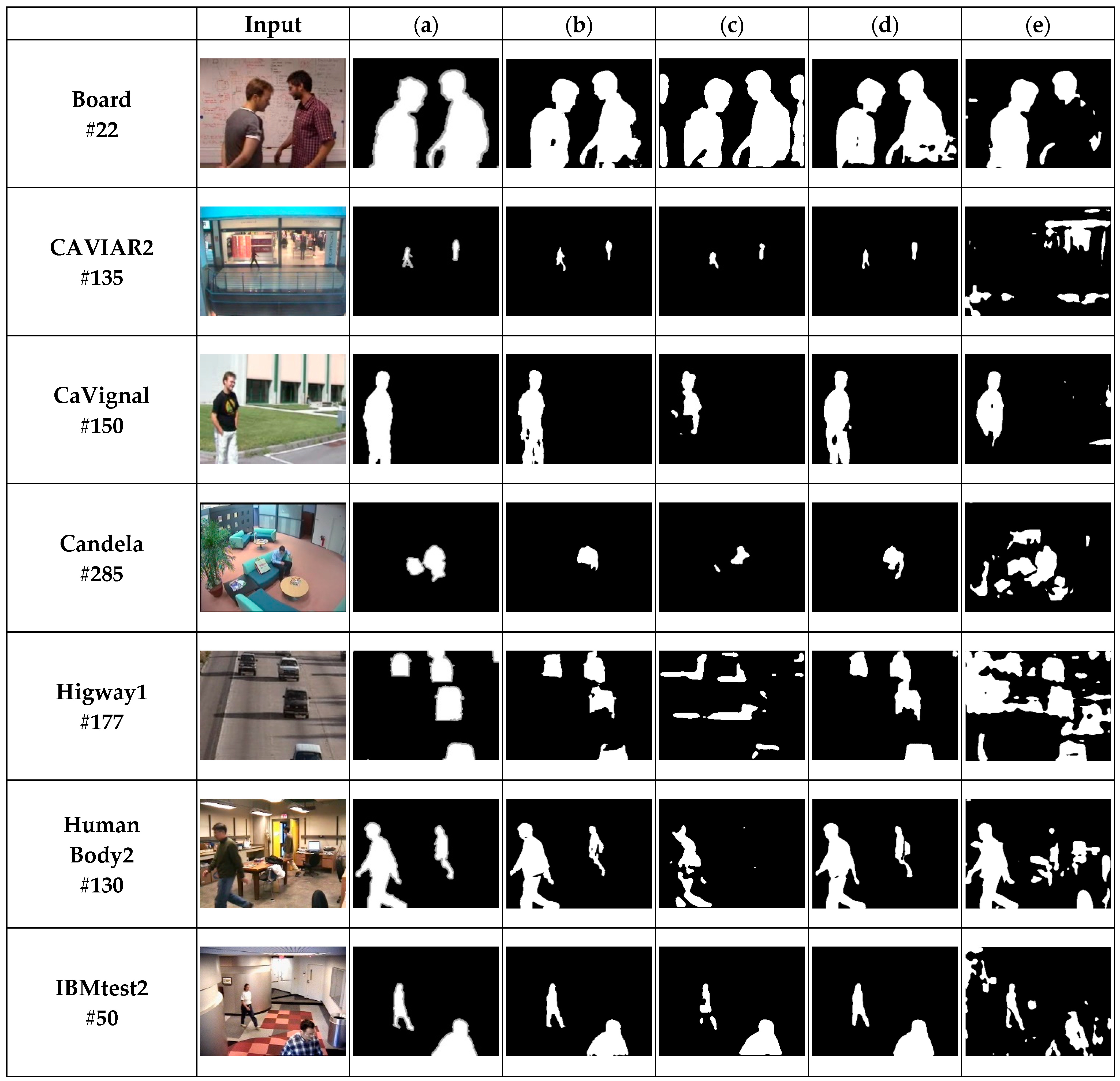
Figure 6 shows some representative results obtained using images in the SBI2015 dataset. We can notice that the proposed algorithm shows more improvement than traditional background model-based algorithms in the SBI dataset compared to the CDnet 2014 dataset. We think that this is caused by the differences in those datasets. The CDnet 2014 dataset provides a preparation section to generate background model images before a test, but the SBI dataset does not provide this. Therefore, background model-based algorithms have difficulties in the generation of good background model images in the first part of the SBI dataset.

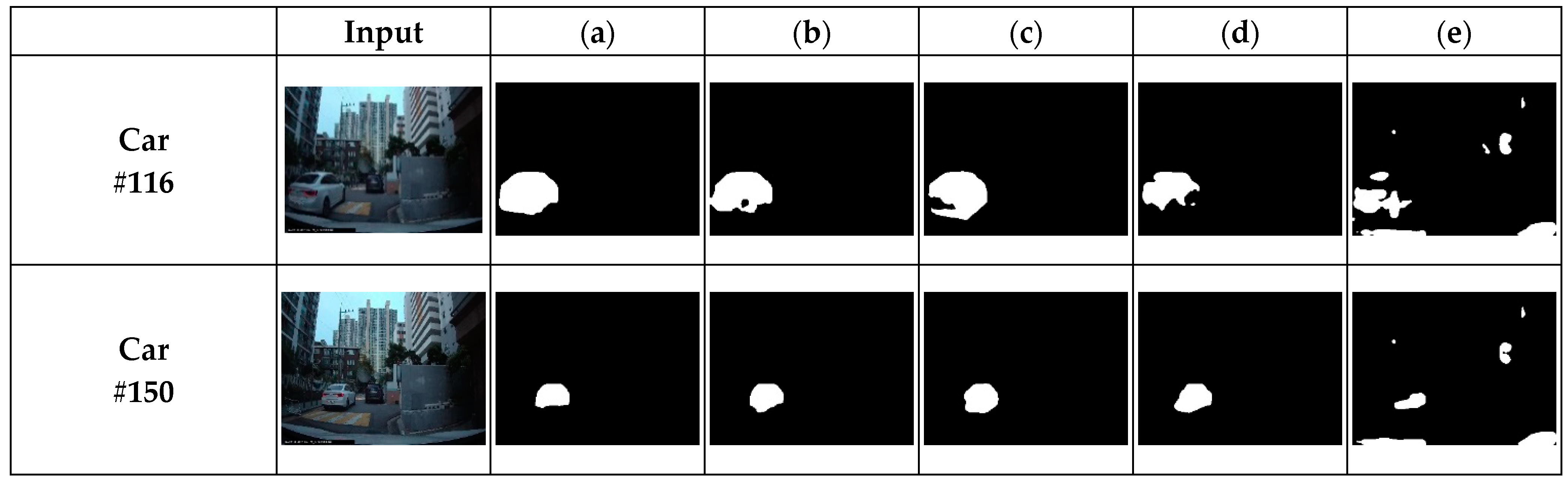
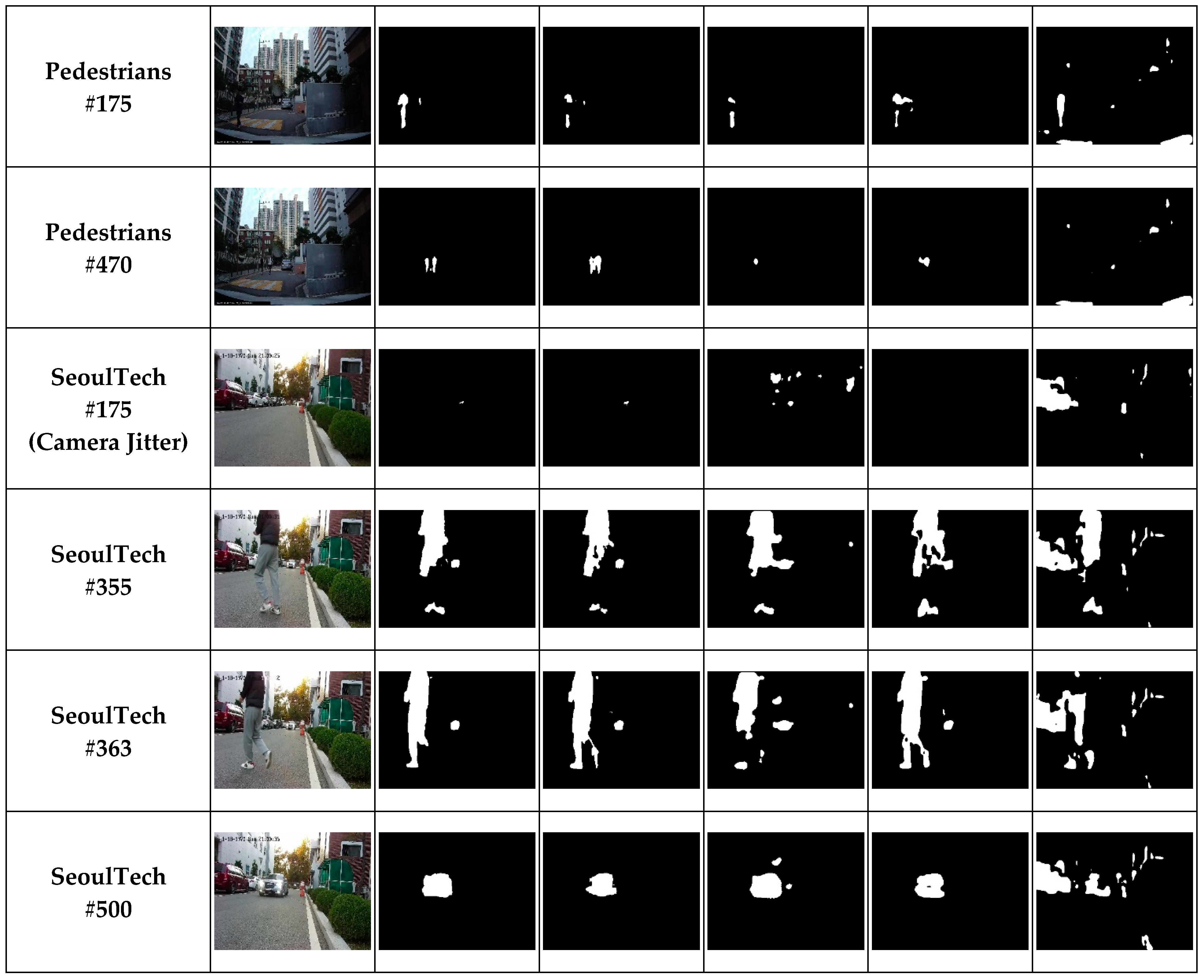
Figure 7 shows the results obtained by using scenes that we acquired ourselves. We only show qualitative results because obtaining a ground truth segmentation map with pixel-wise resolution would requires a huge amount of time. Two sets of results obtained using the proposed method are presented in Figure 7. One was trained using 24 scenes in the CDnet 2014 dataset. The other was trained using 49 scenes in the CDnet 2014 dataset. In Figure 7, the SeoulTech #175 image was acquired with a small jitter of the camera and there are no foreground objects in the scene. Overall, the proposed method trained using 49 scenes achieved better results than when it was trained using 24 scenes. Through this, we can see that if additional datasets can be obtained, better performance can be expected. We can conclude that the proposed method can stably detect foreground objects even in new environments that are not shown in the CDnet dataset.

Deep learning-based algorithms with supervised learning show the best performance in scenes that are similar to training scenes. Therefore, they require training before application to unknown scenes. However, they require a large set of training data. In particular, visual surveillance requires a ground truth segmentation map per pixel, which requires a large amount of time and is high cost. The best option would be a deep learning-based algorithm that does not require training samples of unknown scenes. We want to have an algorithm for visual surveillance that achieves a performance comparable to that of a deep learning-based algorithm, at the same time, requires little effort in preparing samples for training.

The proposed algorithm trained using many samples can achieve better performance than SuBSENSE [2] in situations where there are no training samples. We can conclude that the proposed method achieves better results on scenes that deviate from the training environment, in comparison to traditional and deep learning-based algorithms, from these experimental results. The proposed method is based on deep learning, and it does not require training samples before application to unknown scenes. Our goal is to have a foreground detection algorithm that achieves better performance than traditional unsupervised visual surveillance algorithms. The proposed algorithm meets this requirement by adjusting U-Net to use multiple difference images and training it using multiple scenes.

5. Conclusions

In this paper, we proposed an algorithm that has better generalization power than recent deep learning-based approaches and traditional unsupervised approaches in video surveillance. Using multiple difference images as the input of U-Net and training using all scenes in the CDnet 2014 dataset have made this possible. We demonstrated the improved generalization power of the proposed algorithm through diverse experiments using the CDnet 2014 dataset, the SBI 2015 dataset, and real scenes that we acquired ourselves. We have shown that the generalization ability can be improved by only using multiple difference images as input to other deep learning methods. However, since the frame range of the input data is limited, it is difficult to detect foreground objects that have been stopped for a long time. Additionally, because the proposed algorithm uses multiple difference images as input, it has a shortcoming for scenes acquired by a camera in motion. In further research, we are going to apply recurrent neural networks to cope with these problems. In addition, we plan to do research to cope with the problems that are caused by moving camera using a spatio-temporal network that properly considers spatial and temporal information.

References

- Barnich, O.; Van Droogenbroeck, M. Vibe: A universal background subtraction algorithm for video sequences. IEEE Trans. Image Process. 2011, 20, 1709–1724. [Google Scholar] [CrossRef] [Green Version]
- St-Charles, P.L.; Bilodeau, G.A.; Bergevin, R. Subsense: A universal change detection method with local adaptive sensitivity. IEEE Trans. Image Process. 2015, 24, 359–373. [Google Scholar] [CrossRef]
- Varadarajan, S.; Miller, P.; Zhou, H. Region-based mixture of Gaussians modelling for foreground detection in dynamic scenes. Pattern Recogn. 2015, 38, 3488–3503. [Google Scholar] [CrossRef] [Green Version]
- Wang, Y.; Jodoin, P.M.; Porikli, F.; Konrad, J.; Benezeth, Y.; Ishwar, P. Cdnet 2014: An expanded change detection benchmark dataset. In Proceedings of the IEEE Conference on Computer Vision and Pattern Recognition Workshops, Columbus, OH, USA, 23–28 June 2014; pp. 387–394. [Google Scholar]
- Bouwmans, T. Traditional and recent approaches in background modeling for foreground detection: An overview. Comput. Sci. Rev. 2014, 11, 31–66. [Google Scholar] [CrossRef]
- Sobral, A.; Vacavant, A. A comprehensive review of background subtraction algorithms evaluated with synthetic and real videos. Comput. Vis. Image Underst. 2014, 122, 4–21. [Google Scholar] [CrossRef]
- Garcia-Garcia, A.; Orts-Escolano, S.; Oprea, S.; Villena-Martinez, V.; Garcia-Rodriguez, J. A review on deep learning techniques applied to semantic segmentation. arXiv 2017, arXiv:1704.06857. [Google Scholar]
- Bouwmans, T.; Javed, S.; Sultana, M.; Jung, S.K. Deep neural network concepts for background subtraction: A systematic review and comparative evaluation. arXiv 2018, arXiv:1811.05255. [Google Scholar]
- Stauffer, C.; Grimson, W.E.L. Adaptive background mixture models for real-time tracking. In Proceedings of the IEEE Computer Society Conference on Computer Vision and Pattern Recognition, Fort Collins, CO, USA, 23–25 June 1999; pp. 246–252. [Google Scholar]
- Dempster, A.P.; Laird, N.M.; Rubin, D.B. Maximum likelihood from incomplete data via the EM algorithm. J. R. Stat. Soc. Ser. B (Methodol.) 1977, 39, 1–38. [Google Scholar]
- Elgammal, A.; Duraiswami, R.; Harwood, D.; Davis, L.S. Background and foreground modeling using nonparametric kernel density estimation for visual surveillance. Proc. IEEE 2002, 90, 1151–1163. [Google Scholar] [CrossRef] [Green Version]
- Kim, K.; Chalidabhongse, T.H.; Harwood, D.; Davis, L. Real-time foreground–back- ground segmentation using codebook model. Real-Time Imaging 2005, 11, 172–185. [Google Scholar] [CrossRef] [Green Version]
- Oliver, N.M.; Rosario, B.; Pentland, A.P. A Bayesian computer vision system for modeling human interactions. IEEE Trans. Pattern Anal. Mach. Intell. 2000, 22, 831–843. [Google Scholar] [CrossRef] [Green Version]
- Wang, R.; Bunyak, F.; Seetharaman, G.; Palaniappan, K. Static and moving object detection using flux tensor with split gaussian models. In Proceedings of the IEEE Conference on Computer Vision and Pattern Recognition Workshops, Columbus, OH, USA, 23–28 June 2014. [Google Scholar]
- Bunyak, F.; Palaniappan, K.; Nath, S.K.; Seetharaman, G. Flux tensor constrained geodesic active contours with sensor fusion for persistent object tracking. J. Multimed. 2007, 2, 20–33. [Google Scholar] [CrossRef] [PubMed]
- Evangelio, R.H.; Sikora, T. Complementary background models for the detection of static and moving objects in crowded environments. In Proceedings of the 8th IEEE International Conference on Advanced Video and Signal-Based Surveillance (AVSS), Klagenfurt, Austria, 30 August–2 September 2011; pp. 71–76. [Google Scholar]
- Chen, Y.; Wang, J.; Lu, H. Learning sharable models for robust background subtraction. In Proceedings of the IEEE International Conference on Multimedia and Expo (ICME), Turin, Italy, 29 June–3 July 2015; pp. 1–6. [Google Scholar]
- Sajid, H.; Cheung, S.C.S. Background subtraction for static & moving camera. In Proceedings of the 2015 IEEE International Conference on Image Processing (ICIP), Quebec City, QC, Canada, 27–30 September 2015; pp. 4530–4534. [Google Scholar]
- Hofmann, M.; Tiefenbacher, P.; Rigoll, G. Background segmentation with feedback: The pixel-based adaptive segmenter. In Proceedings of the IEEE Computer Society Conference on Computer Vision and Pattern Recognition Workshops, Providence, RI, USA, 16–21 June 2012; pp. 38–43. [Google Scholar]
- Braham, M.; Van Droogenbroeck, M. Deep background subtraction with scene-specific convolutional neural networks. In Proceedings of the International Conference on Systems, Signals and Image Processing, Bratislava, Slovakia, 23–25 May 2016. [Google Scholar]
- Bilodeau, G.A.; Jodoin, J.P.; Saunier, N. Change detection in feature space using local binary similarity patterns. In Proceedings of the International Conference on Computer and Robot Vision (CRV), Regina, SK, Canada, 28–31 May 2013; pp. 106–112. [Google Scholar]
- Goyette, N.; Jodoin, P.M.; Porikli, F.; Konrad, J.; Ishwar, P. A novel video dataset for change detection benchmarking. IEEE Trans. Image Process. 2014, 23, 4663–4679. [Google Scholar] [CrossRef] [PubMed]
- Babaee, M.; Dinh, D.T.; Rigoll, G. A deep convolutional neural network for video sequence background subtraction. Pattern Recognit. 2018, 76, 635–649. [Google Scholar] [CrossRef]
- Wang, Y.; Luo, Z.; Jodoin, P.M. Interactive deep learning method for segmenting moving objects. Pattern Recognit. Lett. 2017, 96, 66–75. [Google Scholar] [CrossRef]
- Lim, L.A.; Keles, H.Y. Foreground segmentation using a triplet convolutional neural network for multiscale feature encoding. arXiv 2018, arXiv:1801.02225. [Google Scholar]
- Simonyan, K.; Zisserman, A. Very deep convolutional networks for large-scale image recognition. arXiv 2014, arXiv:1409.1556. [Google Scholar]
- Zeng, D.; Zhu, M. Background subtraction using multiscale fully convolutional network. IEEE Access 2018, 6, 16010–16021. [Google Scholar] [CrossRef]
- Zeng, D.; Chen, X.; Zhu, M.; Geosele, M.; Kuijper, A. Background Subtraction with Real-Time Semantic Segmentation. IEEE Access 2019, 7, 153869–153884. [Google Scholar] [CrossRef]
- Braham, M.; Pi’erard, S.; Van Droogenbroeck, M. Semantic background subtraction. In Proceedings of the IEEE International Conference on Image Processing (ICIP), Beijing, China, 17–20 September 2017; pp. 4552–4556. [Google Scholar]
- Sakkos, D.; Ho, E.S.L.; Shum, H.P.H. Illumination-aware multi-task GANs for foreground segmentation. IEEE Access 2019, 7, 10976–10986. [Google Scholar] [CrossRef]
- Patil, P.W.; Murala, S. MSFgNet: A novel compact end-to-end deep network for moving object detection. IEEE Trans. Intell. Transp. Syst. 2018, 20, 4066–4077. [Google Scholar] [CrossRef]
- Varghese, A.; Gubbi, J.; Ramaswamy, A.; Balamuralidhar, P. ChangeNet: A deep learning architecture for visual change detection. In Proceedings of the European Conference on Computer Vision (ECCV), Munich, Germany, 8–14 September 2018. [Google Scholar]
- Akilan, T.; Jonathan, Q.; Safaei, A.; Huo, J.; Yang, Y. A 3D CNN-LSTM-based image-to-image foreground segmentation. IEEE Trans. Intell. Transp. Syst. 2019, 21, 959–971. [Google Scholar] [CrossRef]
- Yang, L.; Li, J.; Luo, Y.; Zhao, Y.; Cheng, H.; Li, J. Deep background modeling using fully convolutional network. IEEE Trans. Intell. Transp. Syst. 2018, 19, 254–262. [Google Scholar] [CrossRef]
- Ronneberger, O.; Fischer, P.; Brox, T. U-Net: Convolutional networks for biomedical image segmentation. In International Conference on Medical Image Computing and Computer-Assisted Intervention; Springer: Cham, Switzerland, 2015; pp. 234–241. [Google Scholar]
- Chollet, F. Keras. 2015. Available online: https://github.com/keras-team/kreas (accessed on 15 February 2021).
- He, K. Delving Deep into rectifiers: Surpassing human-level performance on ImageNet. arXiv 2015, arXiv:1502.01852. [Google Scholar]
- Kingma, D.P.; Ba, J. Adam: A method for stochastic optimization. arXiv 2014, arXiv:1412.6980. [Google Scholar]
- De Gregorio, M.; Giordano, M. A WiSARD-based approach to CDnet. In Proceedings of theBRICS Congress on Computational Intelligence and 11th Brazilian Congress on Computational Intelligence, Ipojuca, Brazil, 8–11 September 2013; pp. 172–177. [Google Scholar]
- Sedky, M.; Moniri, M.; Chibelushi, C.C. Spectral-360: A physics-based technique for change detection. In Proceedings of the IEEE Conference on Computer Vision and Pattern Recognition Workshop, Columbus, OH, USA, 23–28 June 2014; pp. 405–408. [Google Scholar]
- St-Charles, P.L.; Bilodeau, G.A.; Bergevin, R. Universal background subtraction using word consensus models. IEEE Trans. Image Process. 2016, 25, 4768–4781. [Google Scholar] [CrossRef]
- Lim, L.A.; Keles, H.Y. Learning multi-scale features for foreground segmentation. arXiv 2018, arXiv:1808.01477. [Google Scholar] [CrossRef] [Green Version]
- Maddalena, L.; Petrosino, A. Towards benchmarking scene background initialization. In Proceedings of International Conference on Image Analysis and Processing; Springer: Cham, Switzerland, 2015; pp. 469–476. [Google Scholar]
Figure 1.
Use of temporal information by multiple difference images.
Figure 2.
Foreground object detection by U-Net with multiple difference images as input.
Figure 3.
The structure of modified U-Net.
Figure 4.
Test results on scenes used for the training in the CDnet 2014 dataset: (a) ground truth foreground maps, (b) proposed method, (c) SuBSENSE [2], (d) modified FgSegNet-v2, (e) FgSegNet-v2 [42].
Figure 5.
Test results obtained on scenes not used for training in the CDnet 2014 dataset: (a) ground truth foreground maps, (b) proposed method, (c) SuBSENSE [2], (d) modified FgSegNet-v2, (e) FgSegNet-v2 [42].
Figure 6.
Test results on SBI2015 dataset: (a) ground truth foreground maps, (b) proposed method, (c) SuBSENSE [2], (d) modified FgSegNet-v2, (e) FgSegNet-v2 [42].
Figure 7.
Qualitative results on real scenes that were not used in training: (a) proposed method trained using 49 scenes in the CDnet 2014 dataset, (b) proposed method trained using 24 scenes in the CDnet 2014 dataset, (c) SuBSENSE [2], (d) modified FgSegNet-v2, (e) FgSegNet-v2 [42].