Abstract
This paper deals with the digital implementation of a motor control algorithm based on a unified machine model, thus usable with every traditional electric machine type (induction, brushless with interior permanent magnets, surface permanent magnets or pure reluctance). Starting from the machine equations in matrix form in continuous time, the paper exposes their discrete time transformation, suitable for digital implementation. Since the solution of these equations requires integration, the virtual division of the calculation time in sub-intervals is proposed to make the calculations more accurate. Optimization of this solver enables faster runs and higher precision especially when high rotating speed requires fast calculation time. The proposed solver is presented at different implementation levels, and its speed and accuracy performance are compared with standard solvers.
1. Introduction
In the Field Oriented Control (FOC) of electrical machines the rotor flux direction must be known to operate the d-q axis transformation and de-couple the control scheme [1], thus allowing a simple and efficient control strategy. For synchronous machines, the rotor angular position is enough to know the flux direction since it is defined by the magnets, while for induction machines additional information must be collected, implementing what is called a flux observer. In the literature, this function is very well studied, with different types, more or less specific to the machine to control and with different strengths and weaknesses. For example, the sliding mode algorithm [2,3] requires a double integration for currents and fluxes; the Butterworth method presented in [4] present the same double integration plus the need for an additional PI regulator; the dead-beat direct control in [5] is not really ideal for flux estimation, since it looks only at the end torque result; the adaptive model of [6] or, more recently, [7,8] could be very calculation heavy; the methods compared in [9] are just for machines with magnets. Moreover, a flux observer is required for any sensorless application such as permanent magnets [10], reluctance [11], or induction machines [12] that all use the machine equations to find the rotor flux angle, since this operation is intended for applications without the direct measurement of the rotor position and speed.
The importance of a model capable of accurately describing the magnetic status of the machine allows the precise calculation of any quantity linked to the flux, such as the bemf and the torque. A correct flux estimation is the necessary requirement for an effective flux weakening strategy. It can also provide the calculation of the maximum available motor torque that can be conveniently used by the application as given in these articles for electric vehicles application [13], marine propulsion [14] and universal control system [15].
The unified electric model is a formulation of the flux and machine equations that can describe any type of electric machine just by selecting the right parameters. Articles have been written to describe the analytical derivation, its advantages and to show it working on real controls [16]. First introduction of this method and preliminary analysis was introduced in [17].
The use of the unified electric model, as for other approaches, requires the solution of differential equations through integration of the flux, which can be a calculation heavy task. Moreover, to be effective, the estimation of the flux must be available as precise as possible at every PWM cycle, so that the inverter can supply the machine the best voltage to produce the expected performance at each cycle. The flux estimation is only one part of the control scheme that must be completed at each cycle which means that the integration process must use only a fraction of the total time, allowing the other functions such as Field Oriented Control, regulators, modulation and measurement to successfully be carried out.
For machines that present low electric speeds, the integration complexities are not a critical feature, since the flux values change relatively slowly and a low PWM frequency can be used without great disadvantages, thus giving the DSP enough time to conduct calculations. However, in case of high electric speeds, PWM frequencies are kept very high to enable faster and more precise flux variations to extract more performance from the motor, such higher torque, lower ripple or higher dynamic response.
In this case, more speed means higher PWM frequencies and less execution step-time and, often, the limiting factor is the DSP capability to perform the calculation necessary inside the available portion of the PWM cycle. If the calculation frequency is kept low because of hardware limitations, then it means that there are large variation of the machine states during the PWM cycle. Moreover, since the DSP works in discrete time, the discretization introduces intrinsic errors that must be evaluated and minimized.
This paper describes the details of the discrete solver for flux estimation with the optimizations introduced to obtain the best trade off between computational requirements and model precision. Starting from the well known machine equations, execution improvements can be actuated and optimized for discrete-time solvers, such as the ones on Real-Time DSPs [18,19].
The discretization used is the well know Euler backward method, which is simpler than others proposed in [20] such as the Tustin approximation or state-transition method. The trade off for simpler implementation is the accuracy, but this paper introduces a technique to improve it. By dividing the calculation step time in smaller virtual sub-intervals the application of the Euler method is more frequent and higher precision can be achieved without complicating the calculation using, for example, higher order Taylor approximations, such as in [21].
Given that the angular position and fluxes in high speed conditions can change a lot even in between single PWM cycles, the state calculated at the given step can be outdated when its results are actuated in the next cycle. A good approximation of the next step values (prediction) can also be easily implemented [22] using the solution presented, that mitigates this delay phenomenon by predicting the state of the machine for the next cycle.
The solver proposed therefore provides advantages in both execution performance, with few and simple calculations, and great accuracy, thanks to prediction and more precise integration. This is achieved through a simplified iterative integration which has the added advantage of enabling the user to tailor the performance-accuracy trade off depending on the application. Moreover, relying on the Unified Electric Model, the calculation are made with a single implementation modelling all conventional electric machines, thus enabling the use of infinite values for permanent magnets rotor resistance parameters.
To show how the approach can improve both calculation time and accuracy, different models at various stages are compared against each other. First is the continuous model that is taken as reference. Then there is the most common discretization method that substitutes the integration step with a single discrete integration. This is meant to be a good implementation that can run on real-time systems, giving a baseline for speed and accuracy without optimizations. Then the proposed algorithm is used at four different stages of complexity to compare against and showing how it improves both efficiency and accuracy.
The paper uses the Unified Electric Model equations as start because they can represent every conventional machine through just parameter selection, thus giving an optimal field of application. However, since the machine equations and solutions are general for any approach, the subsequent discretizations and optimizations could be simplified or adapted to other interpretations.
Section 2 of this paper describes the machine equations written in the canonical form and their manipulation to get the general Input-State-Output matrix form in the reference frame that keep the values in their respective systems. The next section shows the implementation for a Real-Time controller starting from a simple continuous-time pseudo-code to an optimized discrete-time solution with minimum number of operations. Section 4 will show how these algorithm are implemented in Simulink to conduct speed and accuracy tests. Section 5 shows the results that can be obtained both at slow and high speeds and validates the approach.
2. Unified Electric Machine Model
In this section, the derivation of the basic machine equations is done for an induction machine, but it can be easily expanded to any type of conventional machines [17]. Given the three-phase induction machine of Figure 1, the corresponding stator and rotor equations are (1).
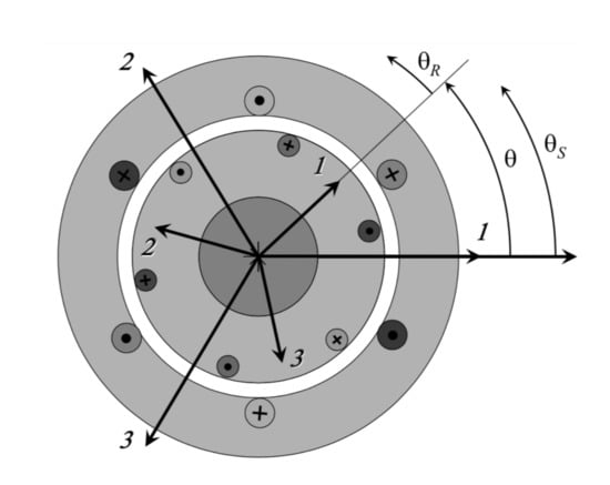
Figure 1.
Three-phase Induction machine example.
Which expand, using the Clarke transformations, into an homopolar component and a complex component, (2). In this work the homopolar component will be disregarded.
Similarly, the rotor and stator phase flux equations can be transformed into their complex form, (3).
where is the coefficient of mutual inductance and and are the stator and rotor auto-inductance respectively.
As said before, (2) and (3) are the general machine equation for an induction machine. However, the same description can be used for all the other types of machines with the appropriate consideration regarding the different rotor fluxes. The structure is identical, but the anisotropy introduces asymmetries in the linked fluxes.
It is easier now to express these equations in a matrix form using the d-q frame convention. Therefore, the stator and rotor voltages, for example, are written as a single column vector such as in (4).
For this paper, the naming convention, given a generic value
is as follows:
- a: subscript that indicates where that value is measured, s for stator, r for rotor, m for mutual;
- b: subscript indicating if the value is referred to the d or q axis;
- c: superscript showing the reference frame that the value is given, s for stator, r for rotor reference frame.
This approach tries to keep all its algorithm into the natural reference frame, which means that every value is given into the reference frame into which it can be measured. This is therefore true when the value has the same letter (s or r) for both the measured position and the reference frame.
In the same way, introducing as the rotor excitation flux matrix, the flux equation becomes (7).
With:
Other than the excitation flux matrix, any machine is described by the two parameter matrices: , or resistance matrix, and , or inductance matrix. They are defined as in (9) and (10), as also described in the relative paper [17], where these matrices have been derived for the Unified Electric Model.
For the correct solution of the equations, all the terms must be referred to the same reference frame, conventionally the rotor is chosen. It is therefore necessary to introduce a transformation to bring stator quantities into rotor frame and vice versa. A rotation of the rotor angle is needed and, since the equations use for elements vectors, a slightly modified Park transformation is used. The matrices that operate the transformation are shown in (11). To simplify the writing, time dependency will be omitted.
- Input: voltage ;
- Output: current ;
- State: flux
Using Park (11) to keep the measurements in the natural reference frame, but operating the necessary conversion to rotor frame, the complete machine equations become (12) and (13).
These equations are completely general for any type of traditional electric machine such as IM, SPM-SM, IPM-SM, R-SM, and AR-SM as shown also in [16,17].
3. Solver Optimization
Since the current Equation (13) is quite straightforward in its use once the flux is known, the focus of the implementation is the flux calculation (12). Also, to keep things more understandable and without compromising the generalization of the results, the machine under consideration is one without excitation flux , such as an induction machine.
3.1. Continuous Time
Using modern simulation environments, it is possible to approximate very well a model solution with infinitesimal step time, as they offer continuous math tools such as Laplace transforms to solve the model. In particular, to calculate the machine flux status an integration must be performed and this is done quite easily with the appropriate integrator function.
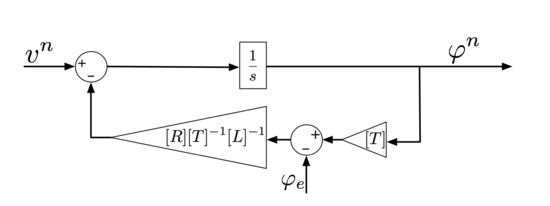
Figure 2.
Implementation scheme for the function calculating the machine flux status.
Any simulation tool such as Simulink offers a discrete library which proposes the corresponding discrete integrator and that can be directly used to get equivalent results. The method proposed in this paper is faster, can be easily made predictive with higher precision, has parameters calculations advantages and it is more suited for embedded applications.
3.2. Discretization
Substituting the flux derivative with its discrete version of difference over time difference, the flux status can be calculated using recursive algorithm every calculation step. Sub-index k indicates the step. Starting from (12), putting and operating some grouping of parameters, the discrete machine equation is (16).
With and the calculation step time.
From here, the recursive step can be evaluate in (17), with the identity matrix.
This algorithm allows the integration of the fluxes, but it contains the time-dependent matrix inversion that is very time consuming. Focusing on this problem, the coefficient can be reworked as in (18).
This approach has two main advantages:
- does not depend on the position , thus it is time invariant in case of constant switching frequency ().
- allows using infinite resistance coefficient for machines with no rotor currents because the matrix is always used as inverse. is diagonal and in case of a coefficient the corresponding element in is simply 0.
3.3. Sub-Interval Predictive Integration
The relevant optimization originally introduced in [17] and here explained in detail, involves the use of an integrating method that divides the calculation step time into smaller ones (sub-intervals) for a more precise calculation without decreasing the step time. Since the integrating values are rotating vectors, the increase in precision is significant, especially at high speed. Moreover, the increase in computation complexity can be limited thanks to the appropriate simplification and reference frame selection.
The (20) can be directly used for the calculation of the flux in k using the form given by (21) or as starting point for the prediction at .
In (22), only the available measured values () and the approximated rotational matrix referred to the next step are used.
As represented in Figure 3, during the interval k, the electrical angle rotates from to . Introducing now the virtual sub-division of k, this rotation is then divided in m sub-intervals. The rotation angle for any sub-interval of k is approximated as (23) by assuming that the rotation in interval k is the same as the previous one.
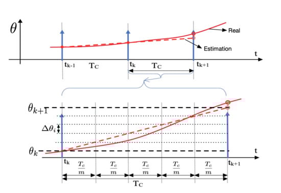
Figure 3.
Discrete time interval sub-division diagram.
The constant rotational matrix valid for each sub-interval in the step k is then calculated as (24).
Given that the rotation at step k is described by , the rotation for a generic sub-interval is . For the property of the rotation matrix the direct and inverse transformation can be expressed as (25).
Additional simplifications can be applied by grouping the calculations in the same reference frame.
So far all the inputs, outputs and states in (27) are kept into their respective reference frames (natural frames). This means that, since the magnetic coupling requires the terms to be into the same reference frame, the stator values are transformed into the rotor reference frame to properly be able to have flux interaction and then transformed back at each sub-interval.
To optimize this step, the general idea is then to make the calculations in the rotor reference frame for the iterations and then transform back in the natural frame only the final results. To illustrate this, (27) is presented again as (28), this time with the reference frames shown explicitly in the superscripts.
Using and :
And then, (30) is derived where voltages and fluxes are both in the rotor reference frame.
Equation (30) is a recursive function that takes the starting voltage, transports it into the rotor reference frame, sum and multiplies the fluxes for the next sub-iteration and finally brings it all back into the natural reference frame at each iteration. This double transformation can be avoided by leaving voltage and flux in the rotor reference frame during the m iterations and transforming just the last results by using the rotational matrix calculated for the cumulative angle increment.
In this way (31) can be isolated from (30), showing just the recursive function for every sub-interval for the rotor flux.
In (31) the integral iteration uses only rotor values (constant in the period ) and, being recursive, the sub-interval angle does not require elevation because it will be achieved by the multiplication by itself in the next sub-interval since the resulting will become .
To note how also the input voltage is rotated to account for the fact that, since in the stator reference frame it is assumed fixed and constant, in the rotor reference frame it is counter-rotating (because the frame rotates).
The final rotation angle can be calculated recursively inside the integration, or outside using (32) depending on which is the less demanding option for the application.
Uniting (31) at the last step m and (32) yields to the last calculation (33) to get the final flux in the k step in the natural reference frame.
The final implementation of any of the above functions on the real motor control would, of course, require an error correction feedback to prevent dangerous integration offsets or erroneous parameters setup and update. Such a system will not be discussed because it is outside the scope of this paper.
It is worth noting that the and matrices are almost diagonal with a very simple calculation of the inverse by changing the sign of the sine elements in position 12 and 21 of the rotational matrix (11).
4. Implementation
Following is the description of the algorithms under testing. To showcase the performance improvements of the optimizations made, intermediate steps of the previously presented equations have been implemented and confronted starting from the continuous model all the way to the optimized discrete algorithm (31) which, the paper argues, is the best compromise for fast, reliable and DSP-optimized integration.
The main outputs of the for loop implementing the integration are the fluxes in the natural reference frames, but intermediate calculation could also be available.
For example, for the calculation of using (25), the elevation of power of can be done recursively at every iteration and the final rotational matrix and its corresponding inverse could be given as output together with the predicted flux. Another approach could be to calculate the final rotational matrix outside the loop by having .
Some implementations presented below already require the elevation of power to occur inside the loop for the proper calculations, so the first method has ben used. However, in the proposed best solution, it has been chosen to use the second approach even though the recursive calculation in the loop could be used. For the testing application, it allows reducing to the minimum the operations inside the for loop, thus increasing the performance especially when incrementing the number of sub-intervals.
Every implementation described has a specific block that minimizes the trigonometric functions for calculating the rotational matrix and its inverse given in (11) by computing only one cosine and one sine both for and .
The parameters used are the resistance matrix , the inverse of the inductance matrix . For the implementations using the matrix , all the machine parameters are hidden inside that matrix, as in (19).
For the sake of simplicity, the implementation refers to an induction machine with magnet flux matrix set to zero and then not shown in these schemes. To show how the implementations would differ for machine with magnets fields, Appendix A shows the full schemes including the representation of the excitation flux.
4.1. CNT: Continuous Model
This function implements directly (12) and the scheme in Figure 2. This model is the best optimized solution for the modelling environment since the program is developed specifically for this type of solver. It does not run real-time, thus making it extremely accurate. This implementation has therefore been chosen as the base reference for precision for the other implementations. Its execution speed has been chosen to normalize the results of the other methods.
4.2. SIMULINK-DSCR: Discrete Model with Simulink Integrator Block
This function is exactly the same as the CNT continuous model, but it uses the Simulink built-in discrete integrator block with forward Euler method that replicates in discrete form the Laplace notation, Figure 4.
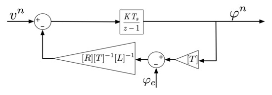
Figure 4.
Discrete time model using built in integrator: SIMULINK-DSCR.
4.3. NAT-DSCR: Discrete Model with Sub-Interval Integration in Natural Reference Frame
The function NAT-DSCR shown in Figure 5 implements (28) using a recursive integration method and a for loop to do the sum of the sub-intervals. It therefore uses all the values in their natural reference frames and multiplies the old rotational matrix with the sub-interval step rotation.
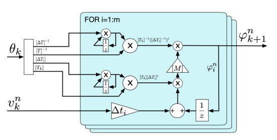
Figure 5.
Discrete time model using the algorithm under study without optimization: NAT-DSCR.
4.4. INV-DSCR: Discrete Model with Fast Matrix Inversion
The function INV-DSCR shown in Figure 6 implements (28) using an approach very similar to NAT-DSCR. The difference is in the calculation of any inverse rotation matrix or . Taking advantage of the fact that the inversion of is the same matrix with just two sign changes, there is a significant simplification by not using a separate calculation of the inverse matrices at every iteration, but just multiplicating for the two elements in position 12 and 21 of (11).
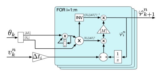
Figure 6.
Discrete time model with fast matrix inversion: INV-DSCR.
Another small improvement is that the calculation of is moved outside the for loop.
4.5. ROTOR-DSCR: Discrete Model with Sub-Interval Integration in Rotor Reference Frame
The function ROTOR-DSCR, shown in Figure 7, implements (31). It represents the sub-integrations done in rotor reference frame and then converts back to the natural frame just the results. This is done using the final rotational matrix directly calculated for the rotation outside of the iterative loop. With this approach the for loop is very much simplified with just a sum and a matrix multiplication between three elements.
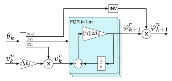
Figure 7.
Discrete time model with rotor reference frame integration: ROTOR-DSCR.
4.6. FAST-DSCR: Discrete Model with Fast Rotation Transformation
The function FAST-DSCR, shown in Figure 8, implements (31) and improves on the previous one by employing a custom matrix multiplication with fewer operations. So far all the matrix multiplications were conducted with the general matrix multiplication rules that use all the elements of the matrices involved. However, matrices and can be considered sparse and their use can be simplified considering only the minimum elements involved. In particular, only the upper left corner of (11) (regarding the stator values) actually operates a rotation with sine and cosine, while the rest of the elements are either 0 or 1, not requiring any mathematical operation.The rotation matrix multiplication is therefore replaced by a much faster custom function that involves only the minimum number of operations indicated in Figure 8 with dotted squares.
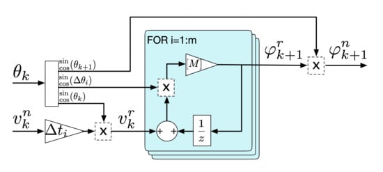
Figure 8.
Discrete time model with fast rotation implementation: FAST-DSCR.
The blocks that in the previous models generated the full rotational matrices are here substituted by similar ones that just output the sine and cosine values.
4.7. Testing Description
To compare performance and accuracy, the different algorithms described above are implemented in the Simulink environment. The comparison is between the different types of integration models that, starting from the voltage and rotation applied to the machine, outputs the fluxes. For this reason, the input side of the model compared is the same, with the generation of an identical voltage source and speed reference.
All of the models have the same parameters, both for the machine simulated and for the solver and inputs. To highlight the possible final application, the machine chosen is an high performance induction machine for electric vehicles, up to 250 kW of power and 15,000 rpm maximum nominal speed, with its main data summarized in Table 1. An IM has been chosen, mainly, because the formulation implies the use of the full 4 × 4 matrix implementation, without simplifications that could be used in SM to improve calculation performances, making it a more complex and severe test-bench.

Table 1.
Simulink general simulation and machine parameters for every implementation used.
To assess how good the discrete approximations presented are to produce the correct machine fluxes, the first comparison is done feeding the model with a symmetric three-phase nominal voltage of 360 V, constant frequency of 6 and the rotor rotating at the same constant speed. The relative low speed and equal value between stator and rotor frequency was chosen to immediately qualitatively give a sense of how good is the implementation since, in a IM, if the speeds are equal, the rotor fluxes are constant. The other testing condition is carried out at an electric speed of to prove both the improvements using increasing sub-intervals integration steps and the algorithm capabilities at high frequency.
Given that the machine equations are known and the continuous implementation is the best approximation possible for a model, its output is chosen as the true one against which the other method are compared. As a remainder, this method cannot be practically implemented in real time DSP, because of the DSP architecture and asynchronous calculation requirements of the method. Moreover, Simulink is optimized to run this type of models, thus producing better performance than any possible discrete-time implementation.
The machine parameters and all the constants needed are calculated by a separate subsystem that takes the user inputs (resistance, inductance, number of iterations, pole pairs and magnet flux) and constructs the required matrices. In particular, it calculates matrix using (19). This division of operation wants to simulate the fact that in the real program some constants can be calculated in different parts of the algorithm to be used by more that one subsystem and that can also run much slower that the main control functions.
Table 1 summarises both the simulation parameters and the machine ones. The entire model is run with a variable-step solver and the discrete algorithms are inserted into a triggered subsystem that produces the requested discrete sample timing.
Figure 9 shows the general setup used for every algorithm under testing. Multiple simulations are run with the same conditions and inputs and the flux outputs are compared afterwards. The simulation only differs inside the block called Model Under Testing where the different models are inserted, which are described in the previous subsections. For the discrete time algorithms the triggering signal is also produced.
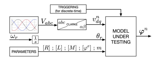
Figure 9.
Model overview used for the tests of the Unified Machine Model.
All the tests are performed by supplying the motor with a standard sinusoidal three-phase voltage with known (variable) frequency. Clarke transformation is operated and the rotor speed is set as a constant.
5. Results
5.1. Model Execution Speed
Execution speed testing are carried out using the parameters in Table 1 and varying the number of sub-interval integrations. Of course the CNT and SIMULINK-DSCR models do not have this variable and their execution time remains constant, apart for a slight improvement between the first and second run, the reason of which is to be found in the Simulink solver engine.
Results are given in Figure 10 normalized with respect to the CNT execution time and the times are found taking the average total running time over 10 simulations. For single sub-interval integration every proposed algorithm is faster than the normal discretization of the SIMULINK-DSCR. Of course, as it will be shown later, the accuracy is not as good. For all the proposed algorithms, then, more than a couple of subdivisions are required in practice to obtain a reasonable accuracy and the calculation manipulation can improve significantly the performance.
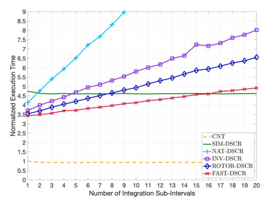
Figure 10.
Execution time comparison increasing the discrete sub-interval integration number. CNT and SIMULINK-DSCR do not depend on the number of sub-intervals. Time is normalized to the CNT execution time.
The NAT-DSCR implementation of Figure 5 uses full transformation matrices, standard inversions and two matrix power elevations all inside the for loop, thus the calculation time increases steeply at the increase of steps. Already at 2 subdivisions the execution time is more than the discrete model SIMULINK-DSCR. The INV-DSCR implementation of Figure 6 that uses a fast inversion technique permits to calculate only one power elevation, therefore the operations inside the loop are reduced significantly and this model is already much faster. Moreover, since the optimization is focused inside the loop, the execution time is much less dependent on the number of sub-intervals.
By following the description of the solvers, the tendency is to move calculations outside of the for loop, thus it can be seen how all the models are quite close at lower steps, while the difference gets bigger increasing the number of sub-intervals. This is what happens in ROTOR-DSCR of Figure 7 where the for loop calculations are substantially simplified.
The best solution described, FAST-DSCR of Figure 8, is still more time efficient than the SIMULINK-DSCR integration process with 15 integration intervals and it is done by having only one matrix multiplication, two sums, one delay and 3 custom simplified matrix transformations.
5.2. Model Precision
This section shows how the different models proposed produce, in fact, very good approximations of the machine flux both at slow and high speeds. The CNT model (Continuous) is used again as the reference output and the others are compared to it. Figure 11 presents, as an example, the outputs of all the models for the machine with rotor turning at the same angular velocity of as the voltage input: the continuous time (CNT), the discrete time with Simulink integrator (SIMULINK-DSCR), the discrete time in natural reference frame (NAT-DSCR), with fast inverse transformation (INV-DSCR), in rotor reference frame (ROT-DSCR) and with fast transformation (FAST-DSCR). The last 4 are all conducted with just 1 sub-interval integration. Overall, it is easy to see how all the models correctly solve the flux equation and give macroscopically equal results.
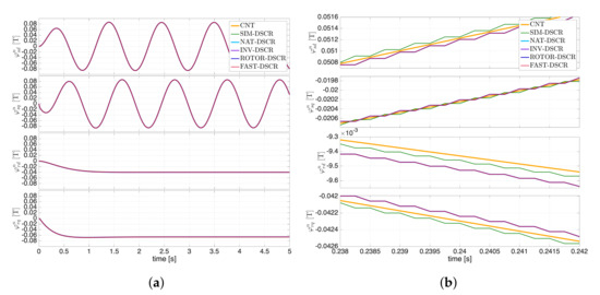
Figure 11.
Simulink flux machine model comparison example between the model presented: CNT, SIMULINK-DSCR, NAT-DSCR, INV-DSCR, ROT-DSCR and FAST-DSCR. (a) overview, (b) zoom to highlight differences.
Figure 11b shows a magnified view of the difference between the CNT solution and the proposed methods. These errors may impact the whole control system since they are predictions used by almost all other functions of the motor control algorithm afterwards and their relative error increases with the flux frequency, thus making it much more problematic at high speeds. As stated before, in the real control system a current error feedback is necessary to compensate for the small integration errors, but it is not described in this paper.
Detailed description and error evaluation is going to be analyzed only for the FAST-DSCR algorithm, given that it has been verified in Section 5.1 that it is the simplest and fastest solver among those proposed. Moreover, since comparing a continuous signal with a discrete one would produce a discontinuous error value, the difference is shown with a very short mean filter (on 2 data points) to better visualize the results.
Since the proposed solution is also a prediction of the flux at the next iteration step , the error is calculated between the current algorithm iteration value and the value at the next step of the CNT model, considered to be the true approximation. This is carried out also for the SIMULINK-DSCR which is not predictive, thus its error is intrinsically larger. However, this decision reflects the ultimate use of the algorithms proposed, which is the best flux estimator for high performance motor control that must implement predictive calculations.
Figure 12 shows the difference between the CNT and FAST-DSCR algorithms as percentage of the maximum value of flux. The error of the SIMULINK-DSCR algorithm is added as a reference. The four plots are for the four fluxes estimated by the model which are the stator and rotor flux in the d and q axis. In this example the rotational speed of the stator field and the electrical angular speed of the rotor are the same and equal to , therefore slow compared to common values.
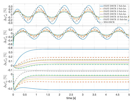
Figure 12.
Percentage difference between CNT and FAST-DSCR at low frequency increasing the integration sub-intervals for flux estimation in (from top to bottom) stator d-axis, stator q-axis, rotor d-axis, rotor q-axis. Stator field and rotor mechanical rotational speed equal to .
The proposed solver is expected to have better accuracy than SIMULINK-DSCR the faster the motor rotation. Therefore Figure 13 shows the error percentage when the stator field rotates at and the rotor has a mechanical angular velocity of , modelling a condition of slip close to the nominal maximum mechanical speed of 15,000 rpm. At this high speed, a clear improvement of the model precision can be seen over the standard integration of SIMULINK-DSCR.
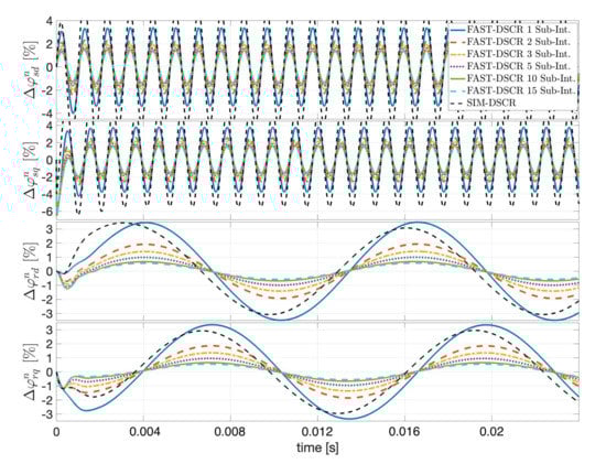
Figure 13.
Percentage difference between CNT and FAST-DSCR at high frequency increasing the integration sub-intervals for flux estimation in (from top to bottom) stator d-axis, stator q-axis, rotor d-axis, rotor q-axis. Stator field and rotor mechanical rotational speed have different values, 6200 and respectively.
To quantify the exact level of improvement, Table 2 shows the mean error squared of the percentage error for the different fluxes and integration methods at both low and high speed. Although the error is always calculated with respect to the CNT solver, in the table the proposed FAST-DSCR method with just 1 integration sub-interval is taken as reference to calculate the percentage improvement of the other instances. The reason behind this choice is to highlight how many sub-intervals are needed for similar accuracy and how much better accuracy can be achieved with the FAST-DSCR compared to the SIMULINK-DSCR.
Table 2.
Mean error squared results of low and high frequency simulations. Base error is the one of the 1 sub-interval model.
As it can be seen in Figure 13 and Table 2, just 1 sub-interval is not enough to justify the speed improvement of FAST-DSCR. Although it performs a little bit better at high speed, the results for the stator flux might be influenced more by the predictive nature rather than true precision. However, increasing the number of integration sub-intervals, a consistent increase in precision is confirmed both in respect to the single interval and to the standard integrator SIMULINK-DSCR.
Precision improvements are also relatively less significant above 5 sub-intervals, improving around 20% from 2 to 5 intervals and only around 10% or less from 5 to 15. In cases where the improvements are comparable with the standard integration SIMULINK-DSCR, namely at low speeds, there is still the advantage of the proposed solver in terms of execution speed. At high speed, however, the FAST-DSCR solver performs much better both in precision and in calculation speed.
Considering both factors, it is verified that the use of the FAST-DSCR solver with a minimum of 5 sub-intervals and a maximum of 10 yields the best compromise between execution speed and precision for most applications.
6. Conclusions
This paper described a fast and reliable way to implement a discrete solver for the flux estimation of any standard AC machine. The proposed solver relies on the Unified Electric Model for AC Machines, because of the versatility of this approach in handling the matrix expressions for any machine type and for its simplicity in discrete time implementation.
Starting from the general machine equations in matrix form, a novel solution for the integration solver is proposed, based on the virtual subdivision of the calculation interval. The paper shows different possible implementations of the computations to introduce inside the for loop for the recursive iterations and outside for non-recursive.
The optimization process, leading to the best configuration of the solver, introduced the recursive algorithm, the subdivision of the integration step in sub-intervals for improved accuracy and then the optimization of the matrix inversions and the selection of the reference frame.
These steps are implemented into a simulation engine to confront the results both in terms of execution speed and precision against a continuous mode solver taken as reference. Multiple algorithms are presented to evaluate the improvement, with the last one called FAST-ROT that uses the for loop in the rotor reference frame, uses a single sine and cosine values for the rotational matrix and calculates most values outside the loop.
Results are shown improving the execution time with the respect to the implementation of the base equation with standard discrete integrators. The FAST-ROT algorithm gives better performance up to 15 sub-intervals and it is a good improvement on the other solutions proposed.
Regarding the precision, error was calculated using the continuous time as reference and taking into consideration that the proposed algorithm is predictive, so the difference is not calculated at the actual calculation interval, but to the next one. The FAST-ROT performs very well at higher speeds, so two examples are brought to validate it both at low and high speeds. In both cases there is a significant improvement increasing the number of sub-intervals and the algorithm gives quantitatively better results than the standard integration method especially at high speed, as expected.
A good balance between execution speed and precision is found to be between 5 and 10 virtual interval sub-divisions and the degree of freedom of this approach allows adapting the algorithm for the target hardware and the specific application.
The subdivision of the calculation step time into virtual sub-intervals, combined with the proposed algorithm, leads to a perfect balance between accuracy and calculation effort, improving over other methods. Thus, this technique is particularly effective when the electrical position of the rotor changes rapidly during the step time. In combination with the control algorithm based on the Unified Electric Model, the proposed solution is suitable for meeting the control requirements in all conventional types of electric motors, particularly in applications with high electrical speeds of rotation or with reduced step times due to the high switching frequencies of the inverter.
Additional tests can be carried out on commercial DSPs to confirm the results and to investigate the real computational weight of the trigonometric functions.
Author Contributions
Conceptualization, C.R.; Formal analysis, C.R.; Investigation, A.P.; Methodology, A.P.; Supervision, A.P.; Validation, M.B.; Visualization, M.B.; Writing—original draft, M.B. All authors have read and agreed to the published version of the manuscript.
Funding
This research received no external funding.
Institutional Review Board Statement
Not applicable.
Informed Consent Statement
Not applicable.
Conflicts of Interest
The authors declare no conflict of interest.
Abbreviations
The following abbreviations are used in this manuscript:
| AC | Alternate Current |
| AR-SM | Assistant Reluctance Synchronous Machine |
| CNT | Continuous Model |
| DSP | Digital Signal Processor |
| FAST-DSR | Discrete model with fast rotation transformation |
| FOC | Field Oriented Control |
| IM | Induction Machine |
| INV-DSCR | Discrete model with fast matrix inversion |
| IPM-SM | Internal Permanent Magnets Synchronous Machine |
| NAT-DSCR | Discrete model with sub-interval integration in natural reference frame |
| PI | Proportional-Integral regulator |
| PWM | Pulse Width Modulation |
| R-SM | Reluctance Synchronous Machine |
| ROTOR-DSCR | Discrete model with sub-interval integration in rotor reference frame |
| SIM-DSCR | Discrete model with Simulink integration block |
| SIMULINK-DSCR | Discrete model with Simulink integration block |
| SM | Synchronous Machine |
| SPM-SM | Surface Permanet Magnets Synchronous Machine |
Appendix A
Machine model schemes with the permanent magnet flux present.

Figure A1.
Discrete time model using the algorithm under study without optimization and PM flux: NAT-DSCR.

Figure A2.
Discrete time model with fast matrix inversion and PM flux: INV-DSCR.

Figure A3.
Discrete time model with rotor reference frame integration and PM flux: ROTOR-DSCR.

Figure A4.
Discrete time model with fast rotation implementation and PM flux: FAST-DSCR.
References
- Liu, G.; Lu, J.; Zhang, H. A Stator Flux-oriented Decoupling Control Scheme for Induction Motor. In Proceedings of the 2007 IEEE International Conference on Control and Automation, Guangzhou, China, 30 May–1 June 2007; pp. 1701–1704. [Google Scholar] [CrossRef]
- Feng, Y.; Zhou, M.; Shi, H.; Yu, X. Flux estimation of induction motors using high-order terminal sliding-mode observer. In Proceedings of the 10th World Congress on Intelligent Control and Automation, Beijing, China, 6–8 July 2012; pp. 1860–1863. [Google Scholar] [CrossRef]
- Lu, Y.; Zhao, J. A sliding mode flux observer for predictive torque controlled induction motor drive. In Proceedings of the 2018 Chinese Control And Decision Conference (CCDC), Shenyang, China, 9–11 June 2018; pp. 3280–3285. [Google Scholar] [CrossRef]
- Fan, S.; Zhou, P.; Zhao, X.; Wang, Z. Novel flux observer based on the butterworth filter for vector control of induction motor. In Proceedings of the 2016 19th International Conference on Electrical Machines and Systems (ICEMS), Chiba, Japan, 13–16 November 2016; pp. 1–5. [Google Scholar]
- Choi, C.; Seok, J.; Lorenz, R.D. Deadbeat-direct torque and flux control for interior PM synchronous motors operating at voltage and current limits. In Proceedings of the 2011 IEEE Energy Conversion Congress and Exposition, Phoenix, AZ, USA, 7–22 September 2011; pp. 371–376. [Google Scholar] [CrossRef]
- Elbuluk, M.; Langovsky, N.; Kankam, M.D. Design and implementation of a closed-loop observer and adaptive controller for induction motor drives. In IEEE Transactions on Industry Applications; IEEE: Piscataway, NJ, USA, 1998; Volume 34, pp. 435–443. [Google Scholar] [CrossRef]
- Belkacem, S.; Naceri, F.; Betta, A.; Laggoune, L. Speed sensorless DTC of induction motor based on an improved adaptive flux observer. In Proceedings of the 2005 IEEE International Conference on Industrial Technology, Hong Kong, China, 14–17 December 2005; pp. 1192–1197. [Google Scholar] [CrossRef]
- Rattanaudompisut, A.; Po-Ngam, S. Implementation of an adaptive full-order observer for speed-sensorless induction motor drives. In Proceedings of the 2015 18th International Conference on Electrical Machines and Systems (ICEMS), Pattaya, Thailand, 25–28 October 2015; pp. 1871–1876. [Google Scholar] [CrossRef]
- Concari, L.; Toscani, A.; Barater, D.; Concari, C.; Degano, M.; Pellegrino, G. Comparison of flux observers for sensorless control of permanent magnet assisted SynRel motors. In Proceedings of the IECON 2016 - 42nd Annual Conference of the IEEE Industrial Electronics Society, Florence, Italy, 23–26 October 2016; pp. 2719–2724. [Google Scholar] [CrossRef]
- Daigavane, M.B.; Vaishnav, S.R.; Shriwastava, R.G. Sensorless Field Oriented Control of PMSM Drive System for Automotive Application. In Proceedings of the 2015 7th International Conference on Emerging Trends in Engineering & Technology (ICETET), Kobe, Japan, 18–20 November 2015; pp. 106–112. [Google Scholar] [CrossRef]
- Yousefi-Talouki, A.; Stella, F.; Odhano, S.; de Lilo, L.; Trentin, A.; Pellegrino, G.; Zanchetta, P. Sensorless control of matrix converter-fed synchronous reluctance motor drives. In Proceedings of the 2017 IEEE International Symposium on Sensorless Control for Electrical Drives (SLED), Catania, Italy, 18–19 September 2017; pp. 181–186. [Google Scholar] [CrossRef]
- Mock, T.; Bimeal, R.; Ling, S.; Comanescu, M. A sensorless induction motor flux observer with inaccurate speed input based on an alternative state-space model. In Proceedings of the 7th IET International Conference on Power Electronics, Machines and Drives (PEMD 2014), Manchester, UK, 8–10 April 2014; pp. 1–6. [Google Scholar] [CrossRef]
- Camacho, E.; Bordons, C. Model Predictive Control, 2nd ed.; Springer: London, UK, 2007. [Google Scholar]
- Tibamoso, K.A.; Oñate, N.A. Model predictive control on induction machine for electric traction. In Proceedings of the 2017 CHILEAN Conference on Electrical, Electronics Engineering, Information and Communication Technologies (CHILECON), Pucon, Chile, 18–20 October 2017; pp. 1–5. [Google Scholar] [CrossRef]
- Li, H.; Xie, H.; Xie, Y. Research on PMSM model predictive control for ship electric propulsion. In Proceedings of the 2018 Chinese Control And Decision Conference (CCDC), Shenyang, China, 9–11 June 2018; pp. 1392–1398. [Google Scholar] [CrossRef]
- Pellegrino, G.; Bojoi, R.I.; Guglielmi, P. Unified Direct-Flux Vector Control for AC Motor Drives. IEEE Trans. Ind. Appl. 2011, 47, 2093–2102. [Google Scholar] [CrossRef]
- Casadei, D.; Pilati, A.; Rossi, C. Unified model and field oriented control algorithm for three-phase AC machines. In Proceedings of the 2013 15th European Conference on Power Electronics and Applications (EPE), Lille, France, 2–6 September 2013; pp. 1–13. [Google Scholar] [CrossRef]
- Samar, A.; Saedin, P.; Tajudin, A.I.; Adni, N. The implementation of Field Oriented Control for PMSM drive based on TMS320F2808 DSP controller. In Proceedings of the 2012 IEEE International Conference on Control System, Computing and Engineering, Penang, Malaysia, 23–25 November 2012; pp. 612–616. [Google Scholar] [CrossRef]
- Xu, G.-K.; Song, P.; Zhao, X.-C. Research on Discrete Model Reference Adaptive Control System of Electric Vehicle. In Proceedings of the 2006 SICE-ICASE International Joint Conference, Busan, Korea, 18–21 October 2006; pp. 2430–2433. [Google Scholar] [CrossRef]
- Hannachi, M.; Soudani, D. Internal model control of multivariable discrete-time systems. In Proceedings of the 2015 7th International Conference on Modelling, Identification and Control (ICMIC), Sousse, Tunisia, 18–20 December 2015; pp. 1–6. [Google Scholar] [CrossRef]
- Inoue, M.; Doki, S. PMSM Model Discretization in Consideration of Park Transformation for Current Control System. In Proceedings of the 2018 International Power Electronics Conference (IPEC-Niigata 2018 -ECCE Asia), Niigata, Japan, 20–24 May 2018; pp. 1228–1233. [Google Scholar] [CrossRef]
- Cortes, P.; Rodriguez, J. Predictive Control of Power Converters and Electric Drives; Wiley: Hoboken, NJ, USA, 2012. [Google Scholar]
Publisher’s Note: MDPI stays neutral with regard to jurisdictional claims in published maps and institutional affiliations. |
© 2021 by the authors. Licensee MDPI, Basel, Switzerland. This article is an open access article distributed under the terms and conditions of the Creative Commons Attribution (CC BY) license (http://creativecommons.org/licenses/by/4.0/).