
Use of Image Correlation to Measure Macroscopic Strains by Hygric Swelling in Sandstone Rocks


University Institute of Physics Applied to the Sciences and Technologies, University of Alicante, P.O. Box 99, 03080 Alicante, Spain
*
Author to whom correspondence should be addressed.
Appl. Sci. 2021, 11(6), 2495; https://doi.org/10.3390/app11062495
Submission received: 15 February 2021
/
Revised: 5 March 2021
/
Accepted: 8 March 2021
/
Published: 11 March 2021
(This article belongs to the Special Issue Nondestructive Testing (NDT): Volume II)
Abstract
:Some materials undergo hygric expansion when soaked. In porous rocks, this effect is enhanced by the pore space, because it allows water to reach every part of its volume and to hydrate most swelling parts. In the vicinity, this enlargement has negative structural consequences as adjacent elements support some compressions or displacements. In this work, we propose a normalized cross-correlation between rock surface texture images to determine the hygric expansion of such materials. We used small porous sandstone samples (11 × 11 × 30 mm3) to measure hygric swelling. The experimental setup comprised an industrial digital camera and a telecentric objective. We took one image every 5 min for 3 h to characterize the whole swelling process. An error analysis of both the mathematical and experimental methods was performed. The results showed that the proposed methodology provided, despite some limitations, reliable hygric swelling information by a non-contact methodology with an accuracy of 1 micron and permitted the deformation in both the vertical and horizontal directions to be explored, which is an advantage over traditional linear variable displacement transformers.
1. Introduction
Hygric swelling is a process that some sandstone rocks undergo when humidity rises. It implies the volume increment of some rock particles, which causes strains, stresses and, depending on the rock composition, a global volume increment in rock. This process can produce small cracks, which is quite a common phenomenon in Europe [1,2]. Consequently, strain measurement due to hygric swelling is an important parameter to assess the suitability of a particular sandstone rock in the construction and restoration of historic buildings.
The most straightforward way to measure hygric swelling is to partially or completely submerge a rock probe in water and measure the vertical displacement of the upper probe boundary with a linear variable displacement transformer (LVDT) [3]. Given the total vertical probe length, and by assuming a zero displacement of its basis, a global vertical strain can be easily calculated as the mean value for all the points on the rock. However, on the one hand, not all points undergo the same strain, and on the other hand, only vertical strains can be measured by this simple procedure. Horizontal swelling measurements by LVDT need more complex devices that are not always suitable for the rock probe under study [4].
Those inconveniences can be overcome by methods based on imaging techniques. Measuring strains by image processing with the proper setup and calculation methods allows the strain to be found for each point in the image according to time [5]. However, image procedures followed to find strains also have some drawbacks. Some are related to the calculation method for tracking a specific detail with time. To this end, the most widely used operation is normalized digital image cross-correlation (DIC), which is implemented herein by the normalized cross-correlation algorithm, normxcorr2, in MATLAB [6]. Although DIC has a nominal accuracy of one pixel, accuracy can increase by subpixel techniques. These techniques consist of interpolating the image or interpolation peak. In both cases, the result is biased toward the nearer integer to, thus, introduce a symmetric error with a sigmoid shape to determine the subpixel position. Some errors may also appear during image recording, such as unexpected camera movements due to mechanical drifts, overheating, changes in ambient light or image distortion due to the camera lens. Therefore, a thorough error study that considers all these factors should be conducted as part of any image procedure.
Image methods for measuring rock swelling have been implemented in very different ways in the literature: generally, probe size determines the most convenient imaging device for acquiring images, ranging from microscope to commercial cameras, and even different image setups can be used for the same probe size. In [7], scanning electron microscope images were used to compare the rock microstructure to the strains measured on a sample of centimeters in size. To measure strains, a 5 Mpx camera with a telecentric lens was used on the same probe side. The resolution for DIC calculation images was 0.5 px/μm. Those images were analyzed by a DIC method developed by [8], which considers the possible cracks that were expected in the analyzed sample. Strains were calculated by displacement derivation using the correlation results. The results showed a very heterogeneous strain distribution during desiccation, probably due to the presence of heterogeneous water and microstructural non-homogenous distribution.
Images directly taken by electron microscopy have also been used to perform DIC strain calculations [9]. In [10], a sample slice (1 mm thick and few millimeters on plane) of an argillaceous rock was recorded during swelling by electron microscopy with a 13.8 Mpx size and a resolution of 0.06 px/μm. The results showed that the macroscopic swelling strain was the combined result of the local free swelling strains and the additional mechanical strains induced by particle interactions. Argillaceous rocks are inhomogeneous materials with different hygric properties that lead to incompatibilities of free-swelling deformations for all its different particles. Additionally, the moisture gradient in the transient state of moisture transport makes some parts swell before others, which confers deformation additional incompatibility. These incompatibilities result in mechanical internal stresses that affect macroscopic local movement during swelling. In summary, previous works have demonstrated that the argillaceous swelling process is substantially affected by non-controllable factors such as particle distribution in the sample or moisture transport distribution, which mean that any swelling experiment is hardly reproducible.
From the marked uncertainty point of view that comes with measuring rock swelling, our approach involved simplifying the procedure to obtain a comparable measure of the macroscopic strain to those obtained by LVDT, but without using complex setups and with the possibility of obtaining strains in both directions.
This paper analyzes the swelling process of an argillaceous rock, with a sample of one centimeter in size and a similar image resolution to the papers herein cited, but by using a simpler setup and image processing methods. Rock expansion was analyzed by changes in the rock surface texture. The movement of texture imposed by swelling was tracked by DIC, applied to six different regions of interest (ROIs) located on the edge of the rock surface. The errors of both the experimental setup and numerical methods were carefully analyzed. Finally, it was possible to obtain the relative deformation in the vertical and horizontal directions, and to observe non-uniform stone deformation depending on the proximity of the ROIs to the wet surface.
Some preliminary results obtained with this study have been presented in [11]. Based on these results, the setup and the calculation method very much improved. Mathematical methods have been discussed in [12], where full access to the code is available.
This manuscript is structured as follows. First, we describe the experimental setup and numerical methods, including the error analysis. The results of the dry and wet experiments, and their discussion, are included in Section 3. Finally, the main results are summarized in the last section.
2. Materials and Methods
2.1. Experimental Setup
In this manuscript, we tested porous sandstone used as a construction and building material. It is composed of quartz and feldspar with a clay-rich matrix with known expansive properties. It presents a connected porosity within the 10–12% range. The rock was cut in rectangular parallelepiped samples (size of 11 × 11 × 30 mm3). In all, four rock samples were tested. In Figure 1, we present a picture of a sample used in our experiments.
Samples were placed in a small container and covered with water up to 1/3 of their height. Water moved by capillarity forces to the top of the samples as with a piston-like imbibition process. As water rose through the sample, it hydrated clay, increased its size and forced rock swelling.
Rock surface images were taken by a color camera Basler acA4600-10uc with a CMOS sensor of 6.5 × 4.5 mm with a Bayer color filter and a spatial resolution of 4608 × 3288 px, being pixel size of 1.4 × 1.4 μm. Since the stone is greyish (see Figure 1), no relevant differences were found between channels, and provided that the green channel is better sampled due to the Bayer filter, only this channel was analyzed herein. However, the other channels were also tested, resulting in similar but noisier results.
A telecentric objective Myutron VTL0513, with the additional VTL05FC lens was used. This objective, together with the lens, provides a magnification of 0.5×. One of the main advantages of using telecentric lenses is that they have a constant non-angular field of view, so they present a significant smaller distortion and field of curvature than conventional lenses. Additionally, the depth of focus value was very low and helped to replace samples in the same exact place. We would like to underline that, since the illumination was controlled by exposition time, the diaphragm was set at its maximum aperture in order to further minimize depth of focus.
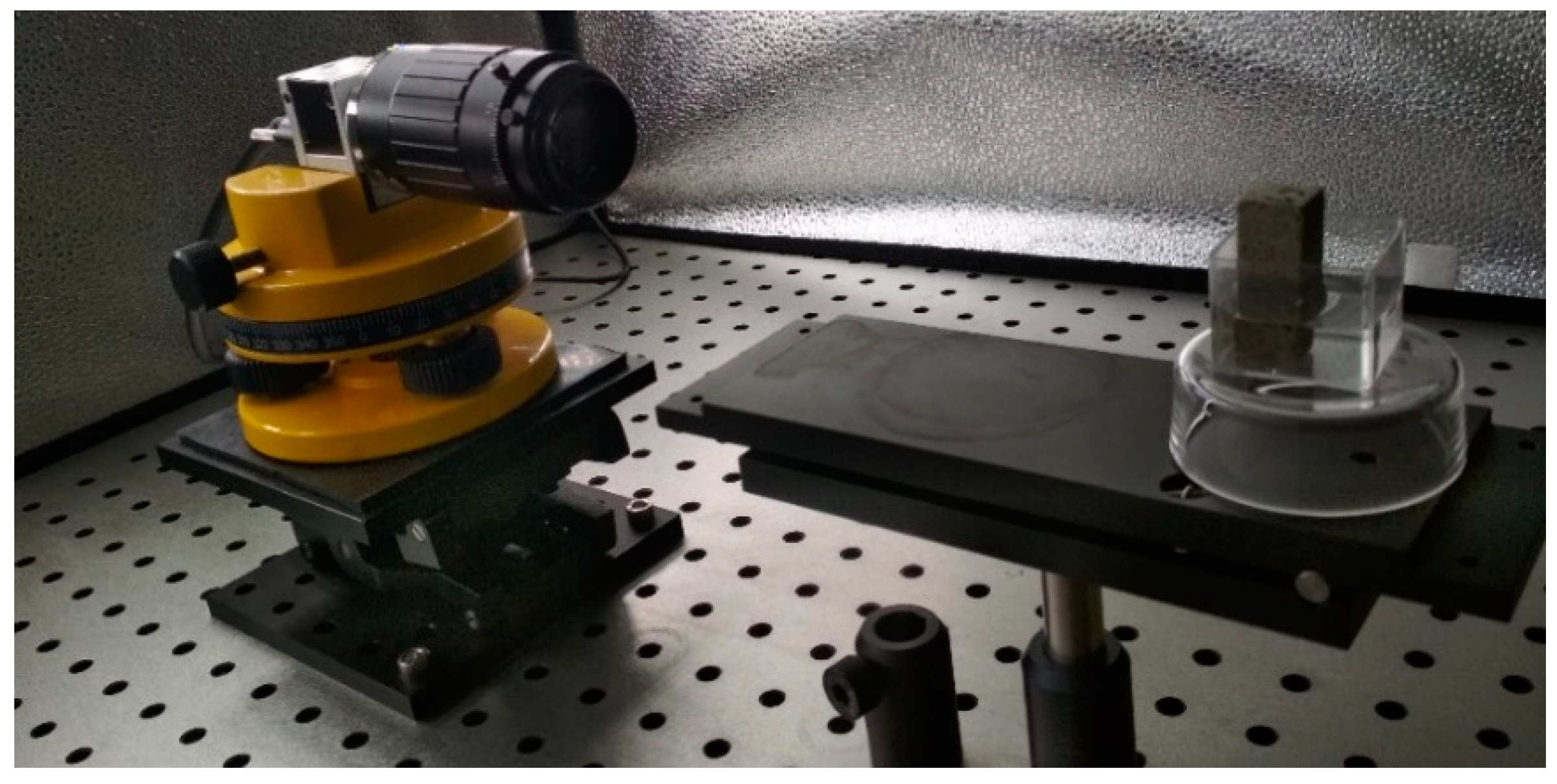
The optical system was centered in the upper part of the probe, thus avoiding the presence of the container border in the image but including both the sample’s lateral borders. The employed magnification, at a working distance of 176 mm (Figure 2), provided a clear image of the rock’s components (Figure 1) with a 0.36 px/μm ratio. Both the sample and image system were placed inside a photo studio light box (Figure 3) to obtain uniform light during the whole experiment and to avoid the influence of air movement on the free water movement through the sample. As it can be seen in the picture, the whole setup was mounted on an antivibratory table. The image brightness, regulated through the artificial light and the exposition time, was adjusted in order to have the maximum contrast, measured through the image histogram.
Before any measurements were taken, the sample was dried in an oven at 50 °C for 1 h. Then, the sample was placed in its position, and the recipient was filled with water using a pipette. After checking that the image was focused, a picture was taken every 2 min for 3 h, so each sequence was composed of a total of 90 images.
2.2. Image Processing Methods
Rock deformation was assessed by surface texture displacements, achieved by calculating the normalized digital image cross-correlation (DIC) between the first frame in the sequence and all the other frames. To increase the accuracy of this result, the correlation peak was interpolated as detailed below [13]. This is a preferred procedure to the other strategy, which consists of interpolating the image itself, as this procedure can induce systematic DIC errors due to inaccurate subpixel image reconstruction [14].
The DIC calculation was not applied to the whole specimen but to some specific ROIs. The size of these ROIs was determined after a texture size analysis by autocorrelation. Different ROIs of fixed sizes were randomly located in 50 different positions on the sample’s surface. Autocorrelation was calculated for each ROI, as was the full width at half maximum of the autocorrelation peak to, thus, estimate the average size of the particles in ROIs. This procedure was repeated for the different ROI sizes, ranging from 5 × 5 px to 200 × 200 px. Figure 4 represents the mean values of the correlation peak of each ROI size for one particular sample and the green channel. Standard deviations are represented as error bars. This figure depicts that small ROIs presented wide variability in detail size, depending on their position, and merely showed sample non-homogeneity. Note that for ROIs larger than 80 × 80, peak width is stable and the variation with ROI location is relatively narrow. A similar graph was obtained for all the samples, with the stability region ranging between 80 and 120 px. Thus, our calculations were performed on ROIs measuring 100 × 100 px for all the samples. Note that the larger ROIs were, the longer the calculation time required, with no clear benefits obtained in quality results terms. Finally, we stress that after some preliminary tests [11], we decided to select the 20 px template smaller than the ROI on both sides to allow texture displacement without going beyond interrogation area limits.
The aim of the method is to determine the macroscopic strains due to hygric swelling. According to this, the deformation has been only calculated in six ROIs of the calculated size at specific positions close to the upper and lateral edges (see Figure 5). Every ROI from each frame was compared by DIC to the corresponding ROI in the same position from the first frame. This distribution allowed us to find the material strain in both the vertical (on both sides of the probe) and the horizontal (at three different heights) directions by using (1).
where is the location of ROI i for time t.
As previously mentioned, the DIC results were refined by interpolating the correlation peak following the procedure explained in [12]. According to the literature, both the interpolation area around the peak and the used fitting function are critical for obtaining accurate results. Two different strategies can be followed: taking a small interpolation area and using a quadratic function as a fitting function, or employing a large area with a Gaussian function. In order to select the best method, we implemented both strategies on the particular rock texture by imposing a synthetic displacement and comparing the results obtained by both methods.
This test was prepared by taking the six ROIs represented in Figure 5 from the first picture of a sequence and numerically displacing by a total of 10 px in the vertical direction in steps of 0.1 px. No horizontal displacement was imposed. The displaced versions were calculated by the Fourier transform shifting property. The synthetic displacement was then compared to the shift obtained by DIC using a quadratic interpolation function in a 3 × 3 neighborhood and a Gaussian fitting function in an 11 × 11 neighborhood around the correlation maximum, according to the recommendations in [12]. The errors found for each ROI are represented in Figure 6, which clearly shows that quadratic fitting of a small neighborhood around the correlation peak was the best strategy.
For the polynomic function, errors were bound, while errors showed no clear trend for Gaussian fits. Note that the errors obtained with Gaussian fitting functions were much larger than polynomic ones. The standard deviation values for polynomic fits were one order of magnitude higher in the direction of displacements than in the other direction, and the maximum value was 0.045 px. As a result of this analysis, a polynomic peak fit with a 3 × 3 neighborhood size was selected for the refinement peak. Finally, Figure 7 summarizes the calculation algorithm that was applied to analyze the samples.
3. Results and Discussion
A final check was performed before continuing with the experiments. It is known that long image acquisition times can imply image distortions due to slight movements of the camera or supporting systems, or sensor deformation due to heat. Therefore, we implemented a “dry” experiment: i.e., the probe was filmed and measured without adding water. From the ROI location for each time, strains were obtained by (1). As the system is supposed to be static, all the obtained shifts may be assigned to experimental errors.
Figure 8 represents the absolute displacement of each ROI from initial position, where we can see a clear drift in the setup, mainly in the vertical direction, which can be up to 15 μm. This behavior was repeated in all the experiments similarly, so this was probably an effect of camera heating, which caused the support to loosen and made the camera move down due to objective weight. Notice also that the results present small instabilities of the order of 0.25 μm or, equivalently, 0.1 px, which is approximately twice the error obtained with the synthetic sequence in the movement direction (see Figure 6). These errors may be due to Gaussian noise in the image and fitting errors in the subpixel calculation algorithms. These fluctuations can be cancelled out by applying smoothing filters in the signal, but since they do not distort the main trend of the result, we preferred to show the data as obtained.
According to these data, our method is not advisable for absolute measurements. However, according to Equation (1), as we were interested in relative positions and strains, it was possible that overall drifting did not affect our results. Figure 9 represents the horizontal and vertical strains obtained for each pair of corresponding ROIs from the images obtained in this dry experiment. Note that in the vertical case, in the same color, we show the strains obtained for each pair of ROIs that are located at the same height, but on different sides of the samples.
Despite experimental instabilities, the method’s accuracy was acceptable with error peak values below 1 × 10⁻³. Mean errors and their standard deviations are presented in Table 1 and Table 2. From them, we take the worst obtained case as the error of this method, which was (0.56 ± 0.16) × 10−3.
It is worth noting that errors in the vertical deformations are slightly larger and more disperse than in the horizontal direction. On the one hand, this may be due to the camera moving, but also to the shorter distance between ROIs. In fact, distance between the lateral ROIs was 3-fold longer than the distance between two consecutive vertical ROIs. As the strain was inversely proportional to the initial position of ROIs, according to Equation (1), the expected error was 3-fold bigger.
Figure 10 depicts the relative displacement measured for all the ROIs in sample 1 during the experiment. Compared to the error graphs in Figure 8, we can see that the displacement measured in the wet experiment was much larger than in the dry experiment. This means that the influence of the error must be considered to be minimum. For the vertical displacement, we see a clear movement due to hydration in the vertical direction. The curve is the typical one that has been observed in other experiments [15], with rapid swelling and a slow stabilization phase. Horizontal displacements were more difficult to interpret as the ROIs on the left and right sides were expected to move in opposite directions. However, the obtained results showed that the movement of all the ROIs went in the same direction, although the displacement of the three ROIs on the left was always less than that on the right. This effect could be due to sample rotation from the irregular expansion of the base or a composition camera drift effect and rock expansion.
In order to better understand this situation, Figure 11 represents the horizontal and vertical strains obtained for all four samples. As strains represent relative displacement between ROIs, all the global effects on the sample (rigid body movements) can be cancelled out, and all the observable effects may be due to internal forces.
As the sample was submerged at the bottom, horizontal swelling was expected to be greater at the bottom than at the upper top. This was observed in all the horizontal displacement graphs, where each pair of ROIs presented minor deformations, because they were further away from water. The observed behavior was similar for all the samples, and the observed variability can be explained by rock non-homogeneity, which can produce samples with slightly different compositions and structures. Note that the upper part of all the samples, which corresponded to ROIs #1 and #4, was much less affected by hygric swelling.
The results for the vertical strains were not so clear. Once again, it would seem that the upper part of samples, which corresponded to the strains between ROIs 1–2 and 4–5 (depicted in blue in Figure 12), were less affected by swelling. The green line, which represents the strains for the ROIs closer to the water level, presented a positive strain during the first 2 h, which means that the rock expanded. After this time, however, the strain decreased, possibly because an early capillary pressure effect was followed by relaxation and water circulation through pores to cause slight shrinkage in the vertical direction but maintained expansion in the horizontal direction. We underline that the strains observed in the vertical directions were of the same order as the peak error limits observed in the dry test (see Figure 9), hence the possibility of the oscillations herein shown not being so marked. However, the trend was very clear, and this behavior was repeated in all four samples with the same shape approximately 2 h after the experiment starts. At that time, as the drift was not as important, the effect cannot be fully explained by experimental errors, and the total displacement in Figure 10 is several orders of magnitude larger than the total displacement observed in the dry experiment (see Figure 8).
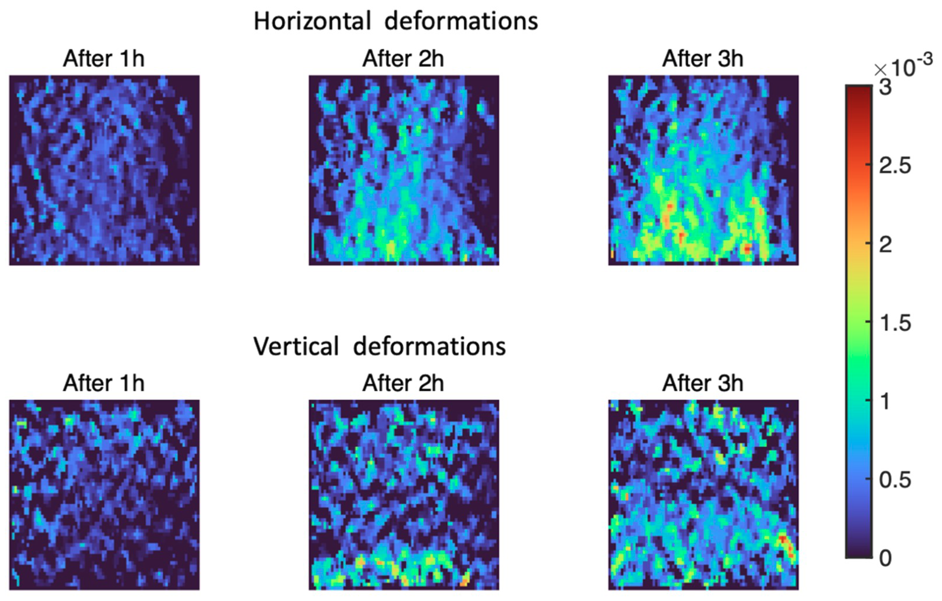
In order to get more insight about the rock behavior, we have calculated different deformation maps of sample 1. In Figure 13, we present the results obtained for the horizontal and vertical deformations at 1, 2 and 3 h after the water addition. To calculate the deformation, the image of the rock has been tessellated in ROIs of 100 × 100 px with an overlapping of 50 px with the adjacent ROIs. Displacement through correlation has been calculated between the corresponding ROIs of the initial picture and the subsequent images. The relative deformation has been obtained between every two alternate ROIs in the considered direction. Finally, in order to avoid outliers and obtain a softer appearance, a 3 × 3 median filter has been applied to the result.
The maps confirm the results in Figure 11 and Figure 12. As it appeared there, the horizontal deformation is stronger than the vertical one. In the horizontal direction, one can see that the lower part of the rock, which is closer to the water surface, suffers a larger dilation than the upper part. In the vertical direction, the effect is not so strong. One can see a clear deformation in the lower part of the sample after 2 h that seems to vanish and spread through all the sample at the end of the experiment.
Note also that the maps show clear inhomogeneities in the distribution of the deformations, which reflects the distribution of particles with different swelling properties through the rock volume.
4. Conclusions
This manuscript discusses a method to measure the deformation of a sandstone rock partially submerged in water due to hygric swelling. This method uses a simple camera and a telecentric objective, which allows macroscopic deformations to be measured. The method uses digital image cross-correlation on small rock areas so that changes in both the vertical and horizontal directions can take place.
Both the numerical and experimental procedures are described, and possible errors were analyzed. According to our calculations, the calculation error method was below 0.1 px or the equivalent to 0.04 μm. Experimental implementation requires long time sequences, which means that marked mechanical and thermal stability conditions are required. In our case, the required stability was not achieved, and an image drift was observed. However, the key parameter in our measurement was strain, which is a relative magnitude, and therefore, rigid body movements did not affect measurements.
Four sandstone rock samples were measured by the herein presented methods. The horizontal strain demonstrated that rock deformation was not uniform, which became larger the closer it was to the submerged part. Our measurements showed a clear dilation in the horizontal direction, which is expected for a partially submerged porous body. The strain measurements in the vertical direction displayed unexpected behavior, so deformation maps at different moments during the experiment were calculated. The maps showed clearly the distribution of the deformations and revealed important inhomogeneities in their distribution, reflecting the composition of the rock.
The method showed good capabilities in measuring local displacement and, from this, the strain of a small rock sample in both the vertical and horizontal directions. The methods herein followed, despite the limitations described, are simpler to implement than those that involve microscopic analyses and may be of much interest for analyzing macroscopic rock dynamics as construction material.
Note that, with the exception of the telecentric lens, which can be replaced by a standard objective with proper distortion calibration, the setup is relatively cheap, which makes this procedure affordable for students or for preliminary tests in research labs. The main drawback of the method is the thermal drift observed. Future works should pay attention to compensate this issue without increasing the price and the complexity of the setup.
Finally, we would like to add that the proposal demonstrates that natural textures can be used as reliable targets for DIC techniques. Further analysis and characterization of textures is needed in order to optimize the subpixel correlation results.
Author Contributions
Conceptualization, D.M. and B.F.; methodology, B.F.; software, D.M.; validation, M.-B.T., D.M. and B.F.; formal analysis, B.F.; investigation, M.-B.T.; resources, B.F.; data curation, D.M.; writing—original draft preparation, B.F.; writing—review and editing, D.M.; visualization, M.-B.T.; supervision, D.M.; project administration, B.F.; funding acquisition, M.-B.T. and B.F. All authors have read and agreed to the published version of the manuscript.
Funding
This research was funded by the Generalitat Valenciana and the European Social Fund (FSE) through the Recruitment of Predoctoral Research Staff ACIF/2018/211 included in the FSE Operational Program 2014–2020 of the Valencian Community (Spain). Belén Ferrer and María-Baralida Tomás acknowledge the support from the Generalitat Valenciana through Project GV/2020/077.
Institutional Review Board Statement
Not applicable.
Informed Consent Statement
Not applicable.
Data Availability Statement
Software for correlation is available at http://rua.ua.es/dspace/handle/10045/110141 (accessed on 15 February 2021). Images or videos of the samples are disposable upon demand.
Acknowledgments
The authors acknowledge David Benavente for providing the rock samples used in the experiments included in this work.
Conflicts of Interest
The authors declare no conflict of interest. The funders had no role in the design of the study; in the collection, analyses, or interpretation of data; in the writing of the manuscript, or in the decision to publish the results.
References
- Di Benedetto, C.; Cappelletti, P.; Favaro, M.; Graziano, S.F.; Langella, A.; Calcaterra, D.; Colella, A. Porosity as Key Factor in the Durability of Two Historical Building Stones: Neapolitan Yellow Tuff and Vicenza Stone. Eng. Geol. 2015, 193, 310–319. [Google Scholar] [CrossRef]
- Colas, E.; Mertz, J.D.; Thomachot-Schneider, C.; Barbin, V.; Rassineux, F. Influence of the Clay Coating Properties on the Dilation Behavior of Sandstones. Appl. Clay Sci. 2011, 52, 245–252. [Google Scholar] [CrossRef]
- Siegesmund, S.; Dürrast, H. Physical and mechanical properties of rocks. In Stone in Architecture; Siegesmund, S., Snethlage, R., Eds.; Springer: Berlin/Heidelberg, Germany, 2011; pp. 97–225. ISBN 978-3-642-14474-5. [Google Scholar]
- Delage, P. On the Thermal Impact on the Excavation Damaged Zone around Deep Radioactive Waste Disposal. J. Rock Mech. Geotech. Eng. 2013, 5, 179–190. [Google Scholar] [CrossRef]
- Sutton, M.A.; Orteu, J.-J.; Schreier, H.W. Image Correlation for Shape, Motion and Deformation Measurements; Springer: Boston, MA, USA, 2009; ISBN 978-0-387-78746-6. [Google Scholar]
- MATLAB; The MathWorks, Inc.: Natick, MA, USA, 2019.
- Fauchille, A.-L.; Hedan, S.; Valle, V.; Prêt, D.; Cabrera, J.; Cosenza, P. Effect of Microstructure on Hydric Strain in Clay Rock: A Quantitative Comparison. Appl. Clay Sci. 2019, 182, 105244. [Google Scholar] [CrossRef]
- Valle, V.; Hedan, S.; Cosenza, P.; Fauchille, A.L.; Berdjane, M. Digital Image Correlation Development for the Study of Materials Including Multiple Crossing Cracks. Exp. Mech. 2015, 55, 379–391. [Google Scholar] [CrossRef]
- Carrier, B.; Wang, L.; Vandamme, M.; Pellenq, R.J.-M.; Bornert, M.; Tanguy, A.; Van Damme, H. ESEM Study of the Humidity-Induced Swelling of Clay Film. Langmuir 2013, 29, 12823–12833. [Google Scholar] [CrossRef] [PubMed]
- Wang, L.L.; Bornert, M.; Yang, D.S.; Héripré, E.; Chanchole, S.; Halphen, B.; Pouya, A.; Caldemaison, D. Microstructural Insight into the Nonlinear Swelling of Argillaceous Rocks. Eng. Geol. 2015, 193, 435–444. [Google Scholar] [CrossRef]
- Ferrer, B.; Tomás, M.B.; Benavente, D.; Mas, D. Use of Image Correlation to Measure Hygric Swelling in Rocks. In Optics, Photonics and Digital Technologies for Imaging Applications VI; Schelkens, P., Kozacki, T., Eds.; International Society for Optics and Photonics: Paris, France, 2020; p. 64. [Google Scholar]
- Tomás, M.-B.; Ferrer, B.; Mas, D. Influence of Neighborhood Size and Cross-Correlation Peak-Fitting Method on Location Accuracy. Sensors 2020, 20, 6596. [Google Scholar] [CrossRef] [PubMed]
- Lei, X.; Jin, Y.; Guo, J.; Zhu, C. Vibration Extraction Based on Fast NCC Algorithm and High-Speed Camera. Appl. Opt. 2015, 54, 8198–8206. [Google Scholar] [CrossRef] [PubMed] [Green Version]
- Schreier, H.W.; Braasch, J.R.; Sutton, M.A. Systematic Errors in Digital Image Correlation Caused by Intensity Interpolation. Opt. Eng. 2000, 39, 2915–2921. [Google Scholar] [CrossRef]
- Benavente, D.; Lock, P.; García del Cura, M.Á.; Ordóñez, S. Predicting the Capillary Imbibition of Porous Rocks from Microstructure. Transp. Porous Media 2002, 49, 59–76. [Google Scholar] [CrossRef]
Figure 1.
Picture of one rock samples. The image has been obtained through the optical setup described in the text.
Figure 1.
Picture of one rock samples. The image has been obtained through the optical setup described in the text.

Figure 2.
Setup for the imaging system and sample.

Figure 3.
Photo studio light box, with one of its sides open.

Figure 4.
Size of the texture details estimated as the autocorrelation FWHM for the different region of interest (ROI) sizes for sample 1 in the green channel at 50 random positions. The results of other channels and samples showed similar outcomes.
Figure 4.
Size of the texture details estimated as the autocorrelation FWHM for the different region of interest (ROI) sizes for sample 1 in the green channel at 50 random positions. The results of other channels and samples showed similar outcomes.

Figure 5.
Number and location of ROIs for which the image processing was done and the direction of the positive displacements.
Figure 5.
Number and location of ROIs for which the image processing was done and the direction of the positive displacements.

Figure 6.
Location errors obtained for all the ROIs using polynomic and Gaussian fits in vertical (left) and horizontal (right) directions.
Figure 6.
Location errors obtained for all the ROIs using polynomic and Gaussian fits in vertical (left) and horizontal (right) directions.

Figure 7.
Flow chart for the image processing used in this work.

Figure 8.
The measured horizontal (left) and vertical (right) shifts for a static dry experiment for each ROI. The results are shown for sample 1, but similar graphs were obtained for all the measured samples.
Figure 8.
The measured horizontal (left) and vertical (right) shifts for a static dry experiment for each ROI. The results are shown for sample 1, but similar graphs were obtained for all the measured samples.

Figure 9.
Measured horizontal (left) and vertical (right) strains for a static dry experiment for each ROI. The results are shown for sample 1, but similar graphs were obtained for all the measured samples.
Figure 9.
Measured horizontal (left) and vertical (right) strains for a static dry experiment for each ROI. The results are shown for sample 1, but similar graphs were obtained for all the measured samples.

Figure 10.
Measured vertical (left) and horizontal (right) shifts for each ROI in a wet experiment. The results are shown for sample 1, but similar graphs were obtained for all the measured samples.
Figure 10.
Measured vertical (left) and horizontal (right) shifts for each ROI in a wet experiment. The results are shown for sample 1, but similar graphs were obtained for all the measured samples.

Figure 11.
Measured horizontal strains for the four hydrated samples.

Figure 12.
Measured vertical strains for the four hydrated samples.

Figure 13.
Deformation maps obtained for sample 1 in horizontal and vertical directions at different moments after the rock immersion.
Figure 13.
Deformation maps obtained for sample 1 in horizontal and vertical directions at different moments after the rock immersion.


Table 1.
Horizontal strain error for a long-term still sequence of the recorded images.
| Horizontal Strain Error (×10−3) | ||
|---|---|---|
| ROIs | MEAN | STD |
| 1–4 | −0.1110 | 0.0411 |
| 2–5 | −0.2163 | 0.0560 |
| 3–6 | −0.4175 | 0.1013 |
Table 2.
Vertical strain error for a long-term still sequence of the recorded images.
| Vertical Strain Error (×10−3) | ||
|---|---|---|
| ROIs | MEAN | STD |
| 1–2 | 0.1167 | 0.1467 |
| 2–3 | 0.1841 | 0.1172 |
| 1–3 | 0.1504 | 0.0833 |
| 4–5 | −0.5586 | 0.1580 |
| 5–6 | 0.0938 | 0.1461 |
| 4–6 | 0.2313 | 0.0823 |
Publisher’s Note: MDPI stays neutral with regard to jurisdictional claims in published maps and institutional affiliations. |
© 2021 by the authors. Licensee MDPI, Basel, Switzerland. This article is an open access article distributed under the terms and conditions of the Creative Commons Attribution (CC BY) license (http://creativecommons.org/licenses/by/4.0/).
Share and Cite
MDPI and ACS Style
Ferrer, B.; Tomás, M.-B.; Mas, D. Use of Image Correlation to Measure Macroscopic Strains by Hygric Swelling in Sandstone Rocks. Appl. Sci. 2021, 11, 2495. https://doi.org/10.3390/app11062495
AMA Style
Ferrer B, Tomás M-B, Mas D. Use of Image Correlation to Measure Macroscopic Strains by Hygric Swelling in Sandstone Rocks. Applied Sciences. 2021; 11(6):2495. https://doi.org/10.3390/app11062495
Chicago/Turabian StyleFerrer, Belén, María-Baralida Tomás, and David Mas. 2021. "Use of Image Correlation to Measure Macroscopic Strains by Hygric Swelling in Sandstone Rocks" Applied Sciences 11, no. 6: 2495. https://doi.org/10.3390/app11062495
Note that from the first issue of 2016, this journal uses article numbers instead of page numbers. See further details here.