High-Precision and Four-Dimensional Tracking System with Dual Receivers of Pipeline Inspection Gauge

Abstract

Pipeline inspection gauges (PIGs) are widely used for nondestructive testing of oil and natural gas pipelines, while above ground markers (AGMs) can locate and track the PIG through a variety of methods, including magnetic flux leakage signals, acoustic signals, and extremely low-frequency (ELF) magnetic signals. Traditional AGMs have the disadvantages of low positioning accuracy and only one-dimensional tracking capability. In this paper, a newly-designed PIG tracking system based on the ELF magnetic field is proposed by assembling dual receivers. Moreover, this paper develops a magnetic field sign-integration algorithm to achieve high-precision and four-dimensional (4-D) tracking of PIG. The simulation and experiment results demonstrate that the tracking system has the capability of 4-D tracking. In comparison with the previously published work, the designed tracking system improves the positioning accuracy and orientation tracking accuracy by more than 50%. The dual receivers tracking system also has the characteristic of high-robustness. Even in the state of lateral offset or tilt, it can still achieve accurate tracking of PIG. The realization of PIG’s high-precision 4-D tracking can improve the accuracy of defect location. Moreover, it can also provide the latest pipeline network layout and facilitate pipeline maintenance and pipeline surveying applications.

1. Introduction

Pipelines are widely used in oil and natural gas transportation projects. Now, the total length of pipelines in a single country may have exceeded ${10}^5$ km [1,2]. However, because pipelines are buried underground for a long time, they may also be corroded [3], even with the typical corrosion prevention techniques (coating, cathodic protection, etc.) [4]. Under the effect of stress–strain, corrosion on the pipe wall gradually evolves into defects [5]. The further development of defects may lead to leakage incidents of the oil or gas, which may cause economic losses and environmental pollution [6]. Based on a series of nondestructive testing technologies such as magnetic flux leakage (MFL) detection [7], eddy current testing [8] and ultrasonic testing [9], the pipeline inspection gauge (PIG) can be developed to detect and evaluate pipeline defects.

The two most important issues in the nondestructive inspection of pipelines are whether defects present and, if so, where they are located [10]. The defect localization is mainly divided into two types: active locating method and above-ground tracking method. In the active locating method, the pipeline inspection gauge (PIG) measures its own movement through the instruments it carries. Furthermore, there are two ways to achieve active locating method, the odometer positioning method [11] and the inertial measurement unit (IMU) method [12,13]. However, due to the slip caused by paraffin oil or the mechanical error caused by wear [10], the positioning error of the odometer can be as high as 10% [14]. What is worse, owing to cumulative counting, there is a cumulative error in the odometer positioning method [15]. Similarly, IMU realizes positioning through the integration of acceleration and angular velocity, and inevitably also has an accumulated error, which is 20 cm per 100 m [16,17]. The inspection mileage of hundreds of kilometers will accumulate positioning errors of hundreds of meters, which is unacceptable in engineering applications.

Therefore, it is necessary to place above-ground markers (AGM) at regular intervals along the pipeline to communicate with the PIG and correct the accumulated error of the active locating method [18]. At present, the most commonly used AGMs are based on the magnetic flux leakage signal, which uses the magnetic field leaking from the permanent magnet carried by the MFL–PIG to achieve the positioning of the PIG [19]. Obviously, it is only applicable to MFL-PIG. The friction between PIG and the pipe wall will generate a self-excited vibration acoustic signal, while the collision between PIG and the pipe weld will generate a transient shock vibration acoustic signal [20]. Therefore, the MEMS acoustic vector sensors can be used in AGMs to track the PIG [21,22]. However, the amplitude of the friction sound is small, which results in a limited propagation distance and a weak anti-interference ability. The amplitude of the collision sound is large, but because of the obstruction of the soil, the specific position of the weld cannot be determined directly on the ground, so the PIG cannot be accurately tracked either [21].

There is also another above-ground tracking method based on an extremely-low frequency (ELF) magnetic field, which has better positioning accuracy and stronger general applicability. PIG carries the transmitter, which can radiate the ELF magnetic field, while the tracking receiver above the ground locates PIG by detecting the ELF magnetic field signal [23]. The AGM based on the ELF magnetic signal has been widely used in practical engineering [24]. It is also suitable for tracking the PIG with unconventional shapes [25]. The most common way to analyze the ELF–AGM is the magnetic dipole model (MDM) method [26]. Qi established a MDM for the PIG transmitter, and proposed the pipeline global position system to realize long-distance tracking of the pipeline based on the principle of multi-satellite measurement [27]. Based on the x-axis and y-axis signals of the magnetic field of the transmitter, Piao gives an orthogonal search coils model, which is applied to the tracking of high-speed PIGs through the least square criterion and ternary decision trees [28,29].

There are three obvious problems with traditional ELF–AGMs. Firstly, the positioning of PIGs has not yet reached centimeter-level accuracy. The positioning error is 40 cm in [27] and 20 cm in [30]. Secondly, both Qi [30] and Piao [28] measure the ELF magnetic field in the axial and radial direction at the same time, which leads to signal redundancy. Thirdly, the traditional AGMs achieve only one-dimensional tracking for PIG (the axial direction of the pipe). However, the terrain above pipelines may change over time, and the actual location of pipelines may be inconsistent with the initial design [31]. Since the actual location of the underground pipeline is unknown, multiple dimensions tracking is required to accurately describe the location of the pipeline—including the relative position $(x,y,z)$ between the tracking receivers and the PIG, and the pitch angle between the pipeline and the ground plane—in the Cartesian coordinate system with the PIG transmitter as the origin and the direction along the pipeline as the z-axis. The coordinate z is used to track the PIG along the pipeline direction. The improvement of the tracking accuracy of the coordinate z can help to improve the accuracy of the defect location. The coordinate x is used to position the lateral offset distance between the PIG and the AGM, while the coordinate y is used to position the vertical distance between the PIG and the AGM, that is, the buried depth of the pipeline. The acquisition of the dimensions x, y, and pitch angle can quantify and compensate for their influence on the coordinate z tracking, which will help improve the robustness of the AGMs and improve the accuracy of defect location. In addition, the accurate lateral offset distance between the AGM and the pipeline obtained from the four-dimensional (4-D) tracking, the actual buried depth of the pipeline, etc., are helpful for the excavation and maintenance of the pipeline. At the same time, 4-D tracking of the pipeline is necessary correction information to compensate for the accumulated errors of the pipeline surveying system [18,32]. Qi uses five receiving coils in a horizontal plane to form a receiver array, which has the function of tracking the PIG in multiple dimensions and further improves the tracking accuracy from 40 cm to 20 cm [30]. However, the tracking of multiple dimensions is not adequately realized in addition to the direction along the pipeline. Furthermore, the receiver array with the five coils on the same horizontal plane is too large to be convenient for field use, which can be seen from the experimental scene in Reference [30].

Therefore, the paper proposes a novel tracking receiver system with only two receiving coils distributed vertically and a corresponding 4-D tracking algorithm, which can achieve high-precision and 4-D tracking of the PIG. The dual receivers will detect the radiated magnetic field from transmitters at different heights. Using these dual magnetic signals and the distance between the dual receivers, it becomes possible to achieve 4-D tracking of the PIG. The tracking algorithm is mainly based on the origin symmetry feature of the radial component of the transmitter’s magnetic field, which has the smallest error in various assumptions of the magnetic analysis. It determines that the tracking error of the algorithm proposed in this paper will be smaller than traditional ELF-AGMs. The algorithm is also proposed to solve the redundancy problem in the previous positioning system. First, the paper introduces the design of the dual receivers tracking system in detail. Then, based on the MDM, three possible cases are presented to discuss the 4-D tracking model and corresponding analytical solutions, which are verified by a finite element model (FEM). Moreover, a 4-D tracking algorithm is developed. Furthermore, physical experiments and filed tests that synthesize three cases are performed. The results of FEM simulation and physical experiments are used to prove that the algorithm is feasible and accurate. Finally, the high robustness of the 4-D tracking algorithm is demonstrated.

2. Method

The design of the dual receivers tracking system and the 4-D tracking model based on the MDM are proposed in this section. The FEM model used to verify the tracking algorithm is also introduced.

2.1. The Design of the Dual Receivers Tracking System

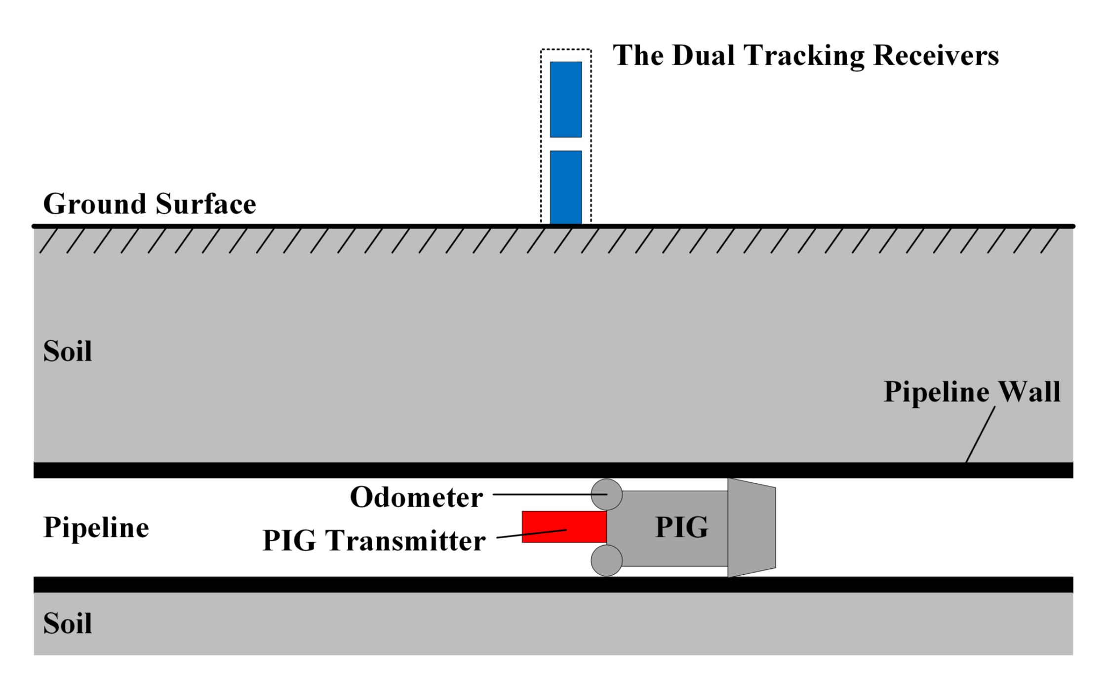
The dual-receiver tracking system is mainly composed of two vertically distributed receiving coils, as shown in Figure 1. In the figure, there is a PIG with a transmitter (the red part) in a pipeline (the black part), while the gray part outside the pipeline is soil. Furthermore, the dual tracking receivers (the blue part) are above the ground.

The tracking system works mainly as follows. First, the transmitter carried by the PIG constantly radiates an ELF magnetic field in the pipeline. The ELF magnetic field reaches the ground through the attenuation of the oil and gas, the pipeline wall, the soil, and the air. Then, the vertically distributed dual tracking receivers detect the magnetic field values at different heights on the y-axis when PIG passes. Last, the tracking system can use the characteristics of the radiation field to track the PIG.

2.2. The Magnetic Dipole Model for Tracking System

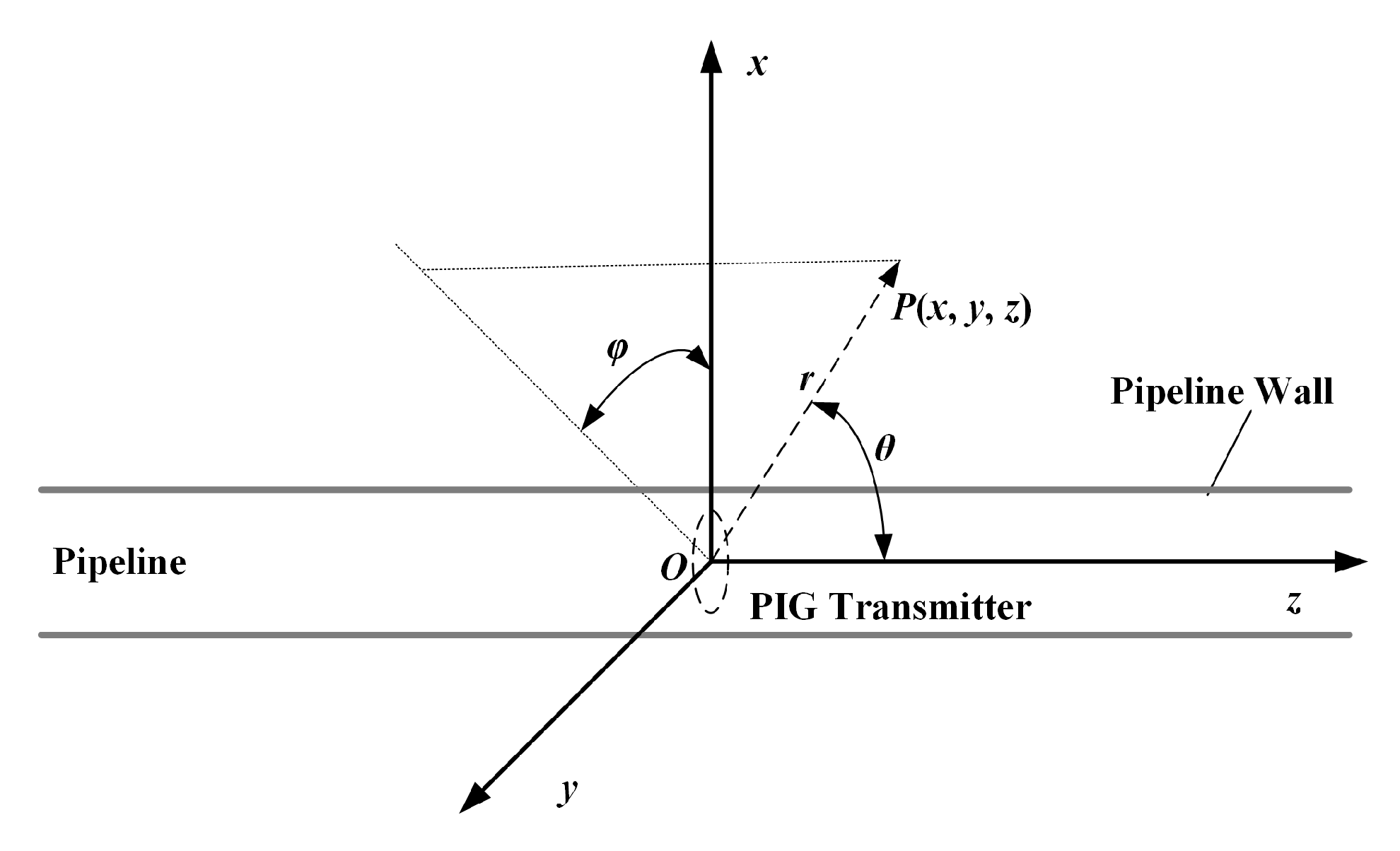
The ELF magnetic field excitation signal of the transmitter is selected as 22 Hz, which has a better penetrating ability for the oil and gas, the pipeline wall, the soil and the air [29,30]. Therefore, the wavelength of the ELF magnetic field is much larger than the diameter of the transmitting coil ($\lambda =\frac{c}{f}$), and each turn of the coil can be regarded as a magnetic dipole as shown in Figure 2. In the figure, the circle part represents one turn of the transmitting coil, and r is the distance from the field point to the magnetic dipole, $\theta$ is the angle between ${\mathbf{e}}_r$ and z-axis and $\phi$ is the angle between ${\mathbf{e}}_r$ and $xOy$ plane.

2.2.1. The Magnetic Dipole Model in Vacuum

Considering that the propagation distance r is much larger than the coil length, the coil can be considered as a superposition of N magnetic dipoles, while N is the number of turns of the transmitting coil. Therefore, in the Cartesian coordinate system, the radiated magnetic field of the transmitting coil can be rewritten as (1):

$$\dot{\mathbf{H}}=\frac{N\dot{I}\mathrm{S}}{4\pi }(\frac{1}{{\left(x^2+y^2+z^2\right)}^{2.5}}+\frac{\mathrm{j}k}{{\left(x^2+y^2+z^2\right)}^2})\left[3xz{\mathbf{e}}_{\mathbf{x}}+3yz{\mathbf{e}}_{\mathbf{y}}+\left(2z^2-x^2-y^2\right){\mathbf{e}}_{\mathbf{z}}\right],$$

(1)

where ${\mathbf{e}}_{\mathbf{x}}$, ${\mathbf{e}}_{\mathbf{y}}$ and ${\mathbf{e}}_{\mathbf{z}}$ are the unit vectors in the Cartesian coordinate system and I is the excitation current in the transmitting coil. The wavenumber is $k=2\pi f\sqrt{{\epsilon }_0{\mu }_0}$, while f is the frequency of the excitation current. ${\mu }_0$ is the permeability of free space, ${\epsilon }_0$ is the permittivity of free space and S is the cross section area of the transmitting coil. It is worth noting that the radiated magnetic field in (1) is the near-field of the MDM, because the burial depth of the pipeline is usually several meters. $kr=\frac{2\pi r}{\lambda }\ll 1$, only the higher powers of $\frac{1}{kr}$ in the radiation magnetic field of the MDM in vacuum need to be retained. Furthermore, the nomenclature of the variables in the equations is listed in the Appendix A.

2.2.2. The Attenuation Effect

Since the ELF electromagnetic signal has a good penetration effect in the soil, air, and oil or natural gas, correspondingly, due to the high magnetic permeability and electrical conductivity, the metal pipe is the main factor for the power loss of the ELF signal [26]. The electromagnetic signal attenuation caused by the classical 10 mm pipe wall thickness is two orders of magnitude larger than the attenuation caused by the classical 2–3 m buried depth in soil [30]. Therefore, the attenuation effect of the ELF electromagnetic signal in the soil, air, and oil or natural gas can be ignored. According to the magnetic field propagation model in the lossy medium [26], the attenuation effect of the pipeline can be expressed as (2):

$$H=H_0{e}^{-\alpha h}{e}^{-\mathrm{j}\beta h},$$

(2)

where $H_0$ and H are the amplitudes of the magnetic field intensity before and after attenuation, respectively. $\alpha$ is the loss factor and meets $\alpha =\sqrt{\pi f\mu \sigma }$, while $\beta$ is the phase constant. h is the thickness of the pipe wall; $\sigma$ is the conductivity of the pipe; $\mu$ is the permeability of the pipe, which follows the BH curve. Furthermore, the nomenclature of the variables in the equations is listed in the Appendix A.

2.2.3. The Induced Voltage in the Receiving Coil

Since the PIG with the ELF transmitter is pushed forward by oil or natural gas in the pipeline, its speed is usually slow. Therefore, the induced electromotive force in the receiving coil approximately meets (3):

$$\dot{e}=-\mathrm{j}2\pi fn{\mu }_e\dot{\mathbf{H}}{S}_c{\mathbf{e}}_{\mathbf{y}},$$

(3)

where n is the number of turns of the receiving coil, while $S_c$ is the cross-sectional area. ${\mu }_e$ is the effective magnetic permeability of the magnetic core in the receiving coil. $\dot{\mathbf{H}}$ is the magnetic field intensity, and only the vertical component of the magnetic field shown in (1) can induce a voltage in the receiving coils, which are placed vertically. Furthermore, the nomenclature of the variables in the equations is listed in the Appendix A. Since the f, n, $S_c$ and ${\mu }_e$ can all be regarded as constants, to simplify the model, analyzing the characteristics of the vertical component of the radiated magnetic field is equivalent to analyze the output voltage of the receiving coil.

2.3. The Four-Dimensional Tracking Model

To explore the feasibility and accuracy of the four degrees of freedom (DOF), x, y, z and pitch angle, the 4-D tracking model is divided into three cases for discussion as shown in Figure 3. In the figure, the distance between dual receivers is r. And $d_1$ and $d_2$ are the distances between the transmitter and the dual tracking receivers in y-axis direction, respectively.

2.3.1. The Normal Case

The normal case assumes that the tracking receivers are located directly above the pipeline, and the pipeline is parallel to the ground, as shown in Figure 3a. References that consider only one-dimensional tracking all assume that AGMs work in the normal case [26,27,28]. It is obvious that distances r, $d_1$ and $d_2$ meet the following relationship:

$$d_2=d_1+r,$$

(4)

Referring to (1) and (2) and taking $x=0$, the radiation magnetic field of PIG transmitter in the normal case can be expressed as (5):

$$\dot{\mathbf{H}}=\frac{3N\dot{I}\mathrm{S}yz}{4\pi }(\frac{1}{{\left(y^2+z^2\right)}^{2.5}}+\frac{\mathrm{j}k}{{\left(y^2+z^2\right)}^2})e^{-\left(\beta +\mathrm{j}\alpha \right)h}{\mathbf{e}}_{\mathbf{y}}.$$

(5)

The integration of the amplitude of the magnetic field intensity in (5) is calculaed with respect to the pipe axis direction and marked as $H_{\mathrm{i}}\left(z\right)$:

$$H_{\mathrm{i}}\left(z\right)=-\frac{N\dot{I}\mathrm{S}}{4\pi }\frac{y}{{\left(y^2+z^2\right)}^{1.5}}{e}^{-\sqrt{\pi f\mu \sigma }h}.$$

(6)

Referring to (5), the amplitude of the magnetic field intensity follows the characteristics of origin symmetry, that is, $H\left(z\right)=-H(-z)$ and $H\left(0\right)=0$. Therefore, $H_{\mathrm{i}}\left(z\right)$ reaches a maximum value at $z=0$ shown as (7). The position corresponding to $z=0$ is where the transmitter is located.

$$H_{\mathrm{imax}}\left(y\right)=-\frac{N\dot{I}\mathrm{S}}{4\pi }\frac{1}{y^2}{e}^{-\sqrt{\pi f\mu \sigma }h}.$$

(7)

To conclude, the maximum value of the magnetic field integration (MFI) in (6) can be used to track the DOF z of the PIG. The method of locating PIG using the maximum value of MFI will be more reliable than using the zero magnetic field point. Because of the existence of noise and the limited accuracy of the sensor, it is difficult to accurately find the zero value of the magnetic field signal.

Furthermore, the maximum value of MFI can also be used to calculate accurately the distance between the transmitter and receivers along the y-axis, that is, the buried depth of the pipeline. Referring to (7), the dual receivers tracking system can obtain two maximum values of MFI, $H_{\mathrm{imax}}\left(d_1\right)$ and $H_{\mathrm{imax}}\left(d_2\right)$. Combining (7) and (4), the distance between the PIG transmitter and the tracking receiver 1 and receivers 2 can be calculated as (8):

$$\left\{\begin{array}{c}{d}_1=\frac{\sqrt{H_{\mathrm{imax}}\left(d_1\right)H_{\mathrm{imax}}\left(d_2\right)}+H_{\mathrm{imax}}\left(d_2\right)}{H_{\mathrm{imax}}\left(d_1\right)-H_{\mathrm{imax}}\left(d_2\right)}r,\\ d_2=\frac{\sqrt{H_{\mathrm{imax}}\left(d_1\right)H_{\mathrm{imax}}\left(d_2\right)}+H_{\mathrm{imax}}\left(d_1\right)}{H_{\mathrm{imax}}\left(d_1\right)-H_{\mathrm{imax}}\left(d_2\right)}r.\end{array}\right.$$

(8)

The magnetic ratio in (8) has its own characteristics of filtering common-mode noise. As an example, for dual tracking receivers, the effects of pipeline wall and soil on the attenuation of ELF magnetic fields are the same, which can be automatically filtered out by the MFI method.

2.3.2. The Lateral Offset Case

However, the normal case is an ideal situation. Considering that the pipeline is underground and invisible, the receivers may be laterally offset from the pipeline when it is placed above the ground. In this lateral offset case, the dual tracking receivers are located above the pipeline, while the axes of the receivers are offset from the transmitter in the x-axis direction, as shown in Figure 3b. Furthermore, the pipeline is parallel to the ground. In the figure, w is the distance between the PIG transmitter and the tracking receivers in the x-axis direction. Referring to (1) and (2), the vertical component of the radiation magnetic field of the PIG transmitter in the lateral offset case can be expressed as (9):

$$\dot{\mathbf{H}}=\frac{N\dot{I}\mathrm{S}}{4\pi }3yz{e}^{-\sqrt{\pi f\mu \sigma }h}{e}^{-\mathrm{j}\beta h}(\frac{1}{{\left(x^2+y^2+z^2\right)}^{2.5}}+\frac{\mathrm{j}k}{{\left(x^2+y^2+z^2\right)}^2}){\mathbf{e}}_{\mathbf{y}},$$

(9)

The difference in the amplitude of the magnetic field intensity is calculated, marked as $H_{\mathrm{d}}\left(z\right)$:

$$H_d\left(z\right)=\frac{NI\mathrm{S}}{4\pi }{e}^{-\sqrt{\pi f\mu \sigma }h}\left(\frac{3y}{{\left(x^2+y^2+z^2\right)}^{2.5}}-\frac{15y{z}^2}{{\left(x^2+y^2+z^2\right)}^{3.5}}\right),$$

(10)

Referring to (9), maximum and minimum values of the magnetic field intensity can be obtained by taking $H_d\left(z\right)=0$. It can be found that the positions corresponding to the maximum and minimum values, the horizontal offset and the vertical distance meet a position-square relationship, shown as (11).

$$z=\pm \frac{\sqrt{x^2+y^2}}{2}.$$

(11)

Therefore, the lateral offset w can be obtained from the dual receivers tracking system, which can obtain two position-square relationships, while $y=d_1$ and $y=d_2$. Combining the (11) and (4), the lateral offset w can be expressed as (12):

$$w_0=\frac{\sqrt{-r^4-{z_1}^4-{z_2}^4+2r^2{z_1}^2+2r^2{z_2}^2+2{z_1}^2{z_2}^2}}{2r},$$

(12)

where $(\ast ,\ast ,z_1)$ and $(\ast ,\ast ,z_2)$ are the positions corresponding to the maximum and minimum values of the magnetic field intensity under the distance $d_1$ and $d_2$, respectively. $w_0$ is the initial calculated value distance between the PIG transmitter and the tracking receivers in the x-axis direction. Furthermore, the nomenclature of the variables in the equations is listed in the Appendix A.

In the case of known lateral offset, the method of the maximum value of MFI can also be used to accurately calculate the vertical distance. The magnetic field measured by tracking receivers in Figure 3b can be considered as the combination of the radial and circumferential components of the original magnetic field in a cylindrical coordinate system, $H_{\mathrm{rd}}$ and $H_{\phi \mathrm{d}}$, as shown in (13).

$$\left(\begin{array}{cc}{H}_{\mathrm{d}1}& \ast \\ \ast & H_{\mathrm{d}2}\end{array}\right)=\left(\begin{array}{cc}{H}_{\mathrm{rd}1}& H_{{\phi }_1}\\ H_{\mathrm{rd}2}& H_{{\phi }_2}\end{array}\right)\left(\begin{array}{cc}sin{\phi }_1& sin{\phi }_2\\ cos{\phi }_1& cos{\phi }_2\end{array}\right),$$

(13)

where ${\phi }_1$ and ${\phi }_2$ are circumferential angles, which are the angles between the x-axis and the line of the transmitter and receivers. Combining the (11) and (12), ${\phi }_1$ and ${\phi }_2$ in Figure 3b can be expressed as $sin{\phi }_1=\frac{d_1}{z_1}$ and $sin{\phi }_2=\frac{d_2}{z_2}$. $H_{\mathrm{d}1}$ and $H_{\mathrm{d}2}$ comprise the magnetic field measured by dual tracking receivers. Referring to Figure 2, it can be found that the $e_{\phi }$ component of the magnetic field is 0, $H_{\phi i}=0$, $i=1,2$. Furthermore, the nomenclature of the variables in the equations is listed in the Appendix A.

Therefore, the radial components of the original magnetic field in a cylindrical coordinate system, $H_{\mathrm{rd}1}$ and $H_{\mathrm{rd}2}$, can be solved inversely. This process can be defined as a compensation calculation from the measured magnetic field to the original magnetic field. At the same time, the radial distance between the dual receivers in the lateral offset case is no longer r, but $r_{\mathrm{new}}$, which is shown as (14):

$$r_{\mathrm{new}}=\sqrt{{w_0}^2+{d_{20}}^2}-\sqrt{{w_0}^2+{d_{10}}^2},$$

(14)

where $d_{10}$ and $d_{20}$ are initial calculated values of $d_1$ and $d_2$, which can be obtained by (11) and (12). Furthermore, the nomenclature of the variables in the equations is listed in the appendix.

To sum up, integrating the compensated magnetic field $H_{\mathrm{rd}1}$ and $H_{\mathrm{rd}2}$, and taking $r_{\mathrm{new}}$ into (8), the distance between the PIG transmitter and the tracking receiver 1 and receivers 2 in the lateral offset case, $d_{r1}$ and $d_{r2}$ can be obtained. Therefore, the lateral offset w and the distance $d_i$ between the transmitter and receivers can be described as (15), in which $i=1$ or 2:

$$\left\{\begin{array}{c}w=\frac{w_0{d}_{r1}}{z_1},\\ d_i=\frac{d_{i0}{d}_{ri}}{z_i}.\end{array}\right.$$

(15)

where w is the calculated lateral offset, while $d_1$ is also the buried depth of the pipeline. Furthermore, the nomenclature of the variables in the equations is listed in the appendix.

2.3.3. The Pitch Angle Case

If it is in the pitch angle case shown in Figure 3c, the receivers are placed perpendicular to the ground, but not perpendicular to the pipeline due to the change of terrain. In the figure, the tracking receiver is located directly above the pipeline with zero lateral offset in the x-axis, and $\alpha$ is the pitch angle between the PIG transmitter axis and the ground plane. The angle between the transmitter and receivers is $(90°-\alpha )$. The magnetic field measured by tracking receivers in this case is the combination of the y-axis and z-axis components of the original magnetic field in the Cartesian coordinate system, $H_{\mathrm{y}}\left(z\right)$ and $H_{\mathrm{z}}\left(z\right)$. Therefore, the amplitude of measured magnetic field intensity $H\left(z\right)$ can be expressed as (16):

$$H\left(z\right)=\left(\begin{array}{cc}{H}_{\mathrm{y}}\left(z\right)& H_{\mathrm{z}}\left(z\right)\end{array}\right)\left(\begin{array}{c}cos\alpha \\ sin\alpha \end{array}\right)=\frac{NI\mathrm{S}}{4\pi }\frac{\left(3yzcos\alpha +\left(2z^2-y^2\right)sin\alpha \right)}{{\left(y^2+z^2\right)}^{2.5}}{e}^{-\sqrt{\pi f\mu \sigma }h}.$$

(16)

It is easy to find that the existence of the pitch angle causes the positions corresponding to the maximum values of MFI not to overlap on the z-axis. Furthermore, the distance difference of the positions corresponding to the maximum value can be defined as $\Delta z$. Therefore, the pitch angle can be expressed as (17):

$$\alpha =arcsin\frac{\Delta z}{r}.$$

(17)

Taking $H\left(z\right)=0$ in (16), the positions corresponding to the maximum values of MFI can be calculated out:

$$z=\left(-\frac{3}{4}tan\alpha +\sqrt{\frac{1}{2}+\frac{9}{16}{\left(tan\alpha \right)}^2}\right)y,$$

(18)

where the pitch angle $\alpha$ can be obtained from (17), y can be regarded as the initial value in y-axis and can obtained from (11). Therefore, after measuring the magnetic field radiated by the transmitter and calculating the position corresponding to the maximum values of MFI, the position of the transmitter can be located according to (18).

To use the MFI method to locate the PIG in the pitch angle case, multiply (1) with the sign function, and it is easy to find that the y-axis component of the original magnetic field in the Cartesian coordinate system meets the characteristics of symmetry along the z-axis, $H_{\mathrm{y}}\left(z\right)\mathrm{sgn}\left(z\right)=H_{\mathrm{y}}(-z)\mathrm{sgn}(-z)$, while the z-axis component meets the characteristics of origin symmetry, $H_{\mathrm{z}}\left(z\right)\mathrm{sgn}\left(z\right)=-H_{\mathrm{z}}(-z)\mathrm{sgn}(-z)$. Therefore, one can integrate the product of measured magnetic field $H\left(z\right)$ in (16) and sign functions to obtain $H_{\mathrm{Isgn}}\left(y\right)$, as shown in (19). It can be found that the z-axis component of the magnetic field in (16) has been integrated to 0. Furthermore, the maximum value in the MFI method is half of the maximum in the magnetic field sign-integration (MFSI) method in (19).

$$H_{\mathrm{Isgn}}\left(y\right)=\int H\left(z\right)\mathrm{sgn}\left(z\right)\mathrm{d}z,$$

(19)

$$r_{\mathrm{new}}=\sqrt{(r^2-{\Delta z}^2)}.$$

(20)

To conclude, the MFSI method can position the dimension pitch angle of the pipeline by (17) and track the DOF z of the PIG by (18). By replacing the maximum value of MFI with $\frac{1}{2}{H}_{\mathrm{Isgn}}\left(y\right)$ and updating the radial distance difference between the dual receivers corresponding with (20), the distance between the PIG transmitter and the tracking receivers in y-axis can be obtained using (8), which is also the buried depth of the pipeline. The MFSI method also works for the normal case and the lateral case, in which the maximum value of MFI can be replaced with $\frac{1}{2}{H}_{\mathrm{Isgn}}\left(y\right)$.

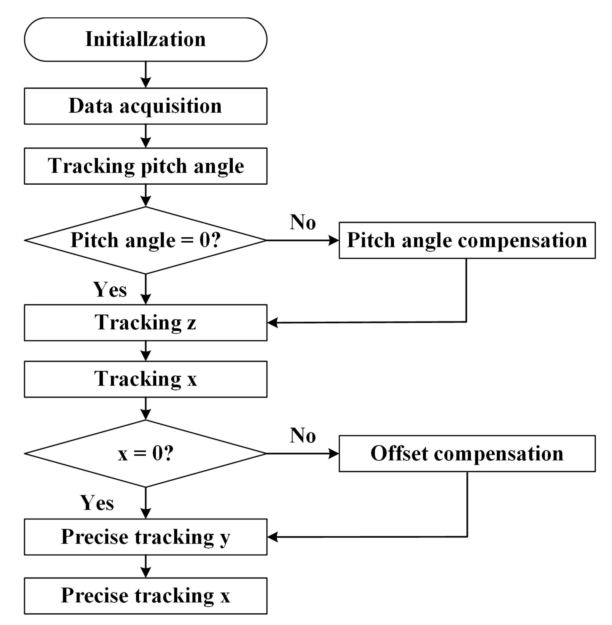
2.4. The Four-Dimensional Tracking Algorithm

In Section 2.3, three possible cases are described in detail, and the solutions of four DOFs are given, respectively. However, the underground pipeline is invisible, and the relative position of the tracking receivers and the pipeline may be one of the above three cases or a combination of the three cases. Therefore, this paper further proposes a comprehensive algorithm to achieve high-precision and 4-D tracking of the PIG in any relative position case. The block diagram of the 4-D tracking algorithm is shown as Figure 4, which is divided into three steps as follows:

• Step 1: The pitch angle of the pipeline is assumed to exist, similar to the pitch angle case. Using (17) and (18), the pitch angle is calculated and the tracking of the DOF z is achieved. (16) is usedto compensate the magnetic field distortion caused by the pitch angle, and the radial distance difference between the dual receivers corresponding with (20) is updated.
• Step 2: The lateral offset of the pipeline is assumed to exist, similar to the lateral offset case. Referring to (11) and (12), the lateral offset is calculated and tracking of the DOF x is achieved. It is worth noting that z in (11) and (12) needs to be subtracted from $\Delta z$ in the solution in Step 1. As in Step 1, the magnetic field distortion caused by the lateral needs to be compensated by (13). The radial distance between the dual receivers needs to be updated with (14).
• Step 3: Referring to (19), the sign-integration of the compensated magnetic field can be obtained. Using the MFSI method in (8) and (15), the tracking of the DOF y is achieved. At the same time, the DOF x can be updated.

Figure 4. Block diagram of the 4-D tracking algorithm.

Figure 4. Block diagram of the 4-D tracking algorithm.

2.5. The Design of the Finite Element Model

To explore the characteristics of the radiated magnetic field of the transmitting coil and verify the MFSI algorithm, a FEM model of the dual receivers tracking system is built as Figure 5. The gray cylinder represents the pipeline, which is made of ferromagnetic material Fe Q235, and its permeability follows the BH curve in the model. The length of the pipeline is 9 m, which is longer than the length of the coil, so the pipe can be considered an infinitely long pipe in simulation. The yellow cylinder represents the transmitting coil with an inner diameter of 20 mm, an outer diameter of 40 mm, a length of 150 mm, and a number of turns of 2500. The amplitude of the excitation current is 1 A, and the frequency is 22 Hz. The black cylinder represents the magnetic core, which is made of Mn-Zn ferrite and has a permeability of 750. The dual blue points represent the measurement point where the dual tracking receivers are located. The goal of the simulation is to analyze the magnetic field characteristics on the line where the points are located. In the figure, $d_1$ is 3 m, $d_2$ is 4 m and r is 1 m.

The simulation is implemented with ANSYS Maxwell, and preprocessing is required before the numerical calculation. The Eddy Current Solver has been chosen due to the sine excitation signal. Different grid sizes are selected in different regions to improve solution accuracy and calculation efficiency. The radiation boundary condition is applied to the model taking into account the characteristics of the radiated magnetic field of the transmitting coil. In addition, the eddy effect of the pipeline is also set in Maxwell.

3. Results

This section gives the results of the FEM simulation, while corresponding physical experiments are designed.

3.1. The Results of the FEM Simulation

The results of the FEM simulation are divided into three cases for discussion.

3.1.1. The Results of the Normal Case

Based on the FEM model as shown in Figure 5, the magnetic fields measured by tracking receivers, shown as Figure 6, are the radiated magnetic fields of the transmitting coil on the line ((0, 3, −4.5), (0, 3, 4.5)) and the line ((0, 3.5, −4.5), (0, 3.5, 4.5)) in meters. It can be found that y-axis components of the magnetic field $B{}_y\left(z\right)$ follow the characteristics of origin symmetry and the z-axis components of the magnetic field $B{}_z\left(z\right)$ follow the characteristics of axisymmetric, which are consistent with theoretical analysis.

References [28,29,30] use orthogonal coils to obtain $B{}_y\left(z\right)$ and $B{}_z\left(z\right)$ at the same time. The zero magnetic field point of $B{}_y\left(z\right)$ and the maximum magnetic field point of $B{}_z\left(z\right)$ are used to locate the PIG. However, the numerical integration of $B{}_y\left(z\right)$ yields $integrationB{}_y$, which has similar characteristics as $B{}_z\left(z\right)$. The maximum values of $B{}_z\left(z\right)$ and $integrationB{}_y$ correspond to the same z-axis coordinates. For the coordinate z tracking of PIG, $B{}_z\left(z\right)$ can be completely replaced by $integrationB{}_y$ in the MFSI method. The effective information obtained by the two orthogonal sensors is the same. A single-axis receiving coil can be used to achieve the same effect as the orthogonal coils. Therefore, the z-axis coil can be omitted. Furthermore, the MFSI tracking algorithm reduces the complexity of the traditional tracking coil system.

According to (8) in the 4-D tracking algorithm, the distance between the PIG transmitter and the tracking receivers can be calculated as in

Table 1. The tracking error of the algorithm in the normal case.

DOF	z	y
MFSI method (cm)	−0.9	298.12
True value (cm)	0.0	300.00
Error (cm)	−0.9	−1.88
Error (%)	-	−0.62

. In the table, the tracking error of the DOF z is −0.9 cm, which is much lower than the error of 14.3 cm in [30] and the error of 40 cm in [27]. At the same time, the tracking error of the DOF y is −1.88 cm, which is also much lower than the error of 20 cm in [30]. In short, the tracking accuracy of the MFSI algorithm is ten times that of traditional ELF-AGMs in the normal case.

3.1.2. The Results of the Lateral Offset Case

Based on the FEM model as shown in Figure 5, the dual tracking receivers have 1 m lateral offset, while $d_1$ is 3 m, $d_2$ is 4 m. Therefore, the magnetic field measured by tracking receivers, shown as Figure 7, are the radiated magnetic field of the transmitting coil on the line ((1, 3, −4.5), (1, 3, 4.5)) and the line ((1, 3.5, −4.5), (1, 3.5, 4.5)) in meter. In a similar manner as the normal case, $B{}_y\left(z\right)$ follows the characteristics of origin symmetry while $B{}_z\left(z\right)$ follows the characteristics of axisymmetric. Furthermore, the coils used for measuring $B{}_z\left(z\right)$ can be omitted by the MFSI method.

In the figure, due to the existence of the lateral offset, there are obvious differences between the measured magnetic field $B{}_{\mathrm{y}1}$ and the original magnetic field $ActualB{}_{\mathrm{y}0}$ in the amplitude and the position corresponding to the maximum amplitude. If the lateral offset is ignored and $B{}_{\mathrm{y}1}$ are used directly like the traditional method, there will definitely be errors in the positioning results.

Referring to (12) and (15), the lateral offset w and the distance between the PIG transmitter and the tracking receivers can be calculated by the MFSI algorithm. Furthermore, the tracking errors are shown in

Table 2. The tracking error of the algorithm in lateral offset case.

DOF	x	z	y
MFSI method (cm)	103.17	0.10	297.52
True value (cm)	100.00	0.00	300.00
Error (cm)	3.17	0.10	−2.48
Error (%)	3.17	-	−0.82

. In the table, the tracking error of the DOF x is 3.17 cm and DOF y is −2.48 cm, which are both much lower than the error of 20 cm in [30]. The tracking error of the DOF z is −0.10 cm, which is also much lower than the error of 14.3 cm in [30] and the error of 40 cm in [27].

3.1.3. The Results of the Pitch Angle Case

Based on the FEM model as shown in Figure 5, there are 30° pitch angles for the tracking receivers, while $d_1$ is 3 m and $d_2$ is 4 m. The magnetic fields measured by tracking receivers, shown as Figure 8, are the radiated magnetic field of the transmitting coil on the line ((0, 3, −4.5), (0, 3, 4.5)) and the line ((0, 3.5, −4.5), (0, 3.5, 4.5)) in meters. Due to the pitch angle, the measured magnetic field is the combination of $H_{\mathrm{y}}$ and $H_{\mathrm{z}}$ of the original magnetic field, and the results in the pitch angle case are different from the two cases discussed earlier. The measured magnetic field $B{}_d\left(z\right)$ does not meet the characteristics of origin symmetry anymore. In addition, there are obvious differences between the measured magnetic field $B{}_{\mathrm{d}1}$ and the original magnetic field $ActualB{}_{\mathrm{d}0}$ in the amplitude and the position corresponding to the maximum amplitude, which can cause high error in positioning methods that directly use data $B{}_{\mathrm{d}1}$. In particular, the position offsets corresponding to the zero magnetic field points of receivers 1 and 2 are 74.10 cm and 48.45 cm, respectively. The offset of the zero magnetic field point will cause an unacceptable error in the traditional ELF-AGMs based on the zero magnetic field point. In contrast, $CompensationB{}_{\mathrm{d}0}$ is the compensated magnetic field by the MFSI method. It can be found that the zero magnetic field point of $CompensationB{}_{\mathrm{d}0}$ has been compensated from 74.10 cm to 10.45 cm, which greatly improves tracking accuracy. The specific results of MFSI algorithm are shown in

Table 3. The tracking error of the algorithm in the pitch angle case.

DOF	Pitch Angle	z	y
MFSI method	29.6038°	−8.17 (cm)	291.83 (cm)
True value	30.0000°	0.00 (cm)	300.00 (cm)
Error	0.3962°	−8.17 (cm)	−7.15 (cm)
Error (%)	1.32	-	−2.38

.

Referring to (17), the pitch angle $\alpha$ can be calculated out. Furthermore, the tracking error of DOF pitch angle is 0.3962°, which is 15 times lower than the error of 6° in [30]. Furthermore, referring to (18) and (8), the DOF z and y are be tracked, whose accuracies are at least twice that of [27,30].

3.2. The Physical Experiments

To verify the MFSI algorithm and the designed dual receivers tracking system, a physical experiment is performed to track a PIG transmitter.

3.2.1. The Design of the Physical Experiment

The designed experiment is a comprehensive case combining the lateral case and the pitch angle case, as shown in Figure 9. Take the forward direction of the transmitter as the z-axis direction and establish a Cartesian coordinate system. The lateral offset of the dual receivers is 0.91 m. $d_1$, the distance in the y-axis between the PIG transmitter and the tracking receiver 1 is 3 m. The distance r between the dual receivers is 0.90 m. The pitch angle $\alpha$ of the dual receivers is 22.885°.

The structure of the PIG transmitter is consistent with the simulation model, and it also includes a coil and a magnetic core, which is marked with a red solid line in Figure 9. The frequency of the excitation current is 22 Hz. To accurately measure the position of the transmitter, the transmitter is not placed in the pipeline during the lab experiment.

Coils in dual tracking receivers wound around a cylindrical core made of Mn-Zn Ferrite. The geometric dimensions of the coils and cores are shown in

Table 4. The geometric dimensions of the tracking receivers.

	Shape	Inner Diameter	Outer Diameter	Length
Coil	Hollow Cylinder	35 mm	38 mm	180 mm
Core	Cylinder	0 mm	35 mm	200 mm

. Coils are made of copper wire with a diameter of 0.2 mm and a number of turns of 3600.

Due to the attenuation effect of the pipeline and the large burial depth of the pipeline, it can be seen from the theoretical calculations and simulation results that the magnetic field intensity at the receiver is much lower than the geomagnetic field. Therefore, the signals received from the tracking receivers need to be preprocessed by a signal processing circuit, which is implemented as the printed circuit board (PCB) in Figure 9. As shown in Figure 10, the signal processing circuit is mainly used for amplification and filtering the measured magnetic field signals and contains five modules. The preamplifier and amplifier module both amplify the weak signal detected by the receivers, and the total amplification of the two modules is 10,000 times. Both amplifiers use high-precision instrumentation amplifiers from Analog Devices. The two bandpass filter modules mainly filter out environmental interference and circuit noise. Their center frequency $f_0$ is 22 Hz, and the bandwidth $f_{\mathrm{bw}}$ is 3 Hz, so the quality factor is 7.33. The bandstop filter is mainly used to deal with the power frequency electromagnetic interference caused by various instruments in the laboratory environment. To improve the quality factor and reduce the bandwidth, all filters use the state variable filter. In Figure 10, the output signals of the Receiver PCB are screenshots of the oscilloscope during the actual measurement process. In contrast, the effective signal amplitude of the signal received by the tracking receiver is too small to be directly observed without signal processing. Therefore, the received signal shown in the figure is actually the signal received when the transmitter and receiver are only 0.1 m apart, mainly to show the characteristics of the received original signal and not equal to the actual detected signal by the dual receivers in experiments.

Altogether, the tracking receivers system consists of two parts, the dual receiving coils, and the Receiver PCB. The coils detect the radiated magnetic field, while the Receiver PCB performs signal preprocessing. Finally, the results are displays by an oscilloscope (Tek MSO64-6-BW-2500). The tracking receivers system is powered by a DC power supply.

3.2.2. The Results of the Physical Experiment

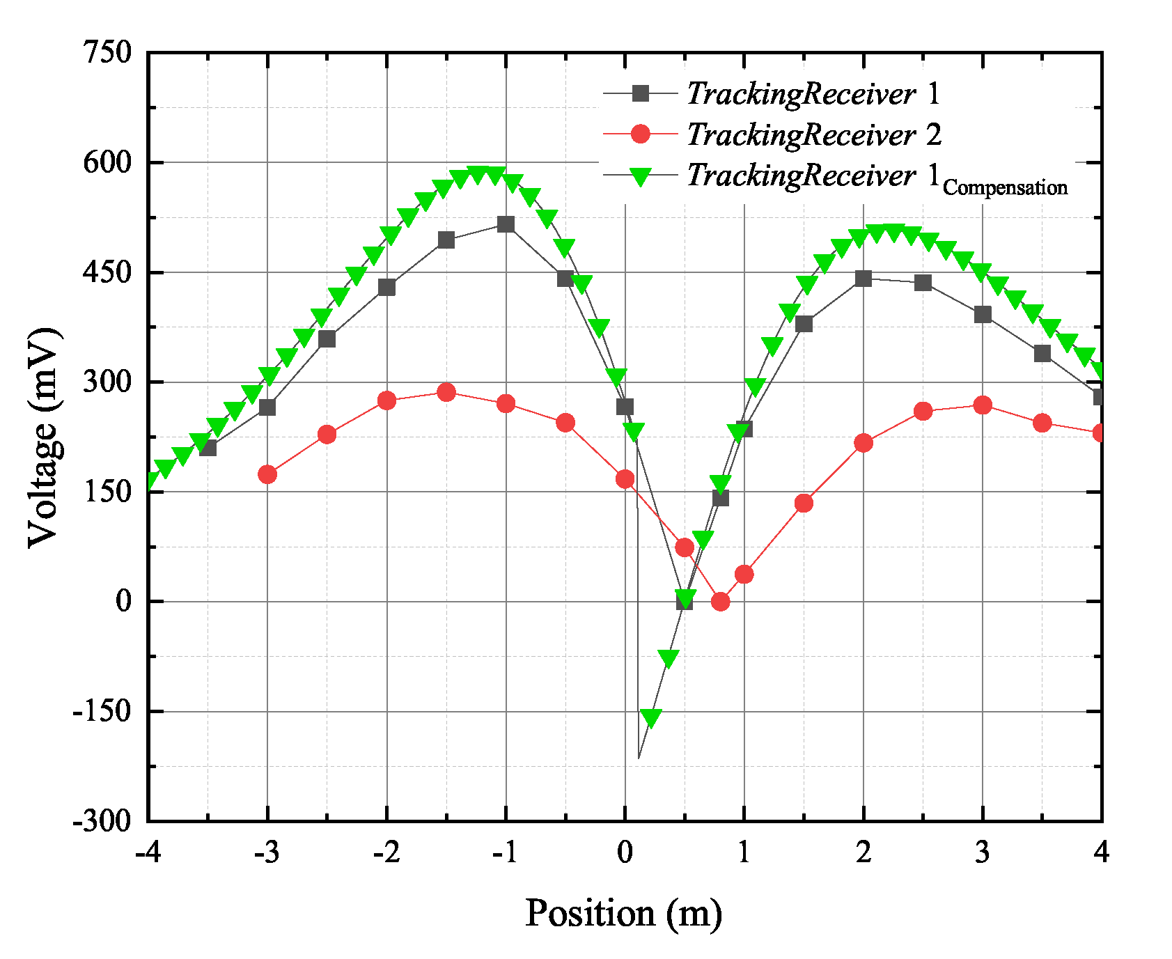
Based on the experimental site as shown in Figure 9, the transmitter moves along the z-axis from −4 m to +4 m. The magnetic field measured by tracking receivers is shown in Figure 11. Similar to the simulation results shown in Figure 8, it can be found that the measured magnetic field by tracking receivers no longer meets the characteristics of origin symmetry due to the pitch angle. Furthermore, there are obvious errors in the amplitude, the position corresponding to the maximum amplitude, and the position of the zero-magnetic field, which will definitely cause errors in tracking for the methods using the measured data directly.

Using the 4-D tracking algorithm based on MFSI shown as Figure 4, the specific results of the experiments are shown in

Table 5. The tracking error of the algorithm in the pitch angle case.

DOF	Pitch Angle	x	z	y
MFSI method	19.519°	91.00 (cm)	−6.95 (cm)	294.95 (cm)
True value	22.885°	100.31 (cm)	0.00 (cm)	300.00 (cm)
Error	−3.365°	−9.31 (cm)	−6.95 (cm)	−5.05 (cm)
Error (%)	−14.70°	−9.28	-	−1.68

. In the table, it can be found that the pitch angle and the lateral offset are all calculated out, the measured magnetic field is compensated and tracking of the DOF x, y, z and pitch angle are all achieved. Furthermore, the error of −3.365° in orientation and the error within 10 cm in locating are more accurate than 6° and 20 cm in [30] and 40 cm in [27], as shown in Table 5.

According to the relationship between the measured magnetic field and the original magnetic field shown in (13) and (16), the magnetic field distortion caused by the pitch angle and the lateral offset can be compensated in sequence. The compensated magnetic field $TrackingReceiver1{}_{\mathrm{compensation}}$ is shown as Figure 11. It can be found that the zero magnetic field point of the compensated magnetic field has been compensated from 80.07 cm to 10.23 cm, which proves that the positioning accuracy has been greatly improved compared to the measured magnetic field $TrackingReceiver1$ and $TrackingReceiver2$.

3.3. The Field Tests

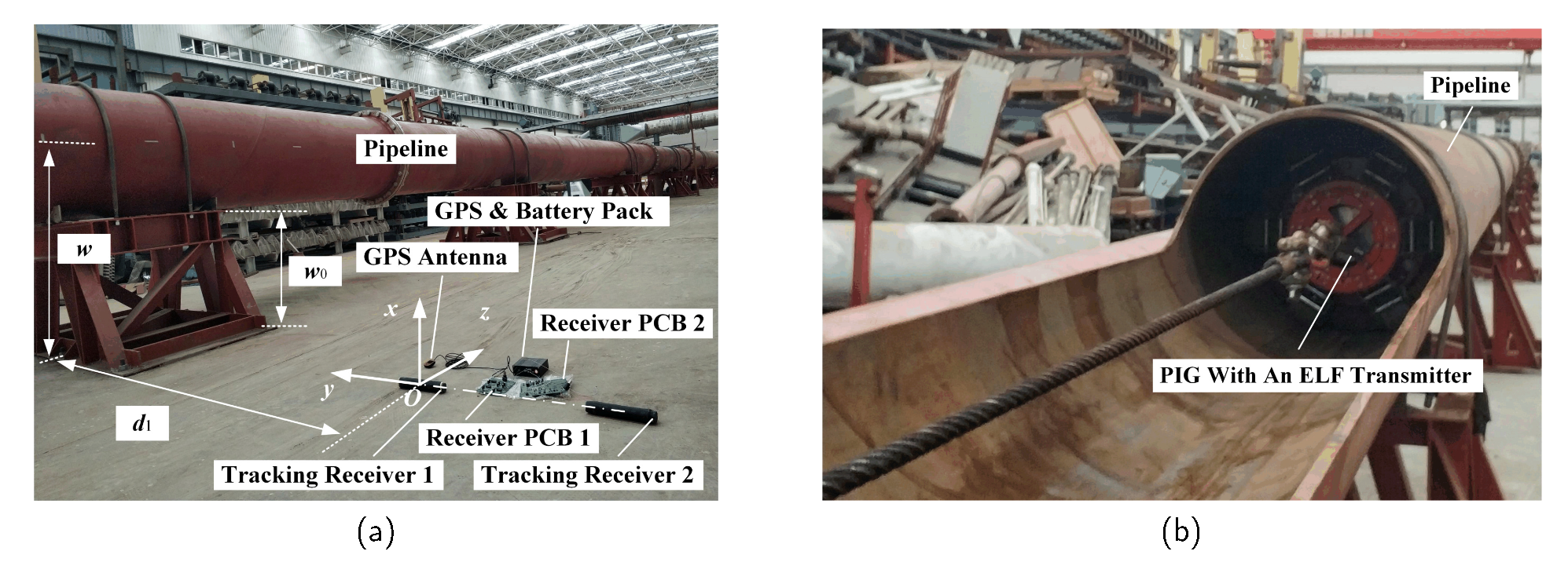
To verify the practical application capabilities of the dual receivers tracking system, we further implemented a series of field tests. As shown in Figure 12, a PIG with the ELF transmitter was pulled forward at a constant speed through the pulling system. The length, wall thickness, and diameter of the oil and gas pipeline are 84 m, 12 mm and 813 mm, respectively. The geometrical and electromagnetic parameters of the transmitter and receivers are the same as those in Section 3.2. The coordinate system is established with the Tracking Receiver 1 as the origin to realize the 4D tracking of the PIG. In this experiment, DOF x represents the height distance between the transmitter and the receiver, and the base height of the pipe is $w_0$ = 800 mm, so $w_1$ = 1187.5 mm. DOF y represents the horizontal distance, while $d_1$ = 1906.5 mm. DOF z describes the tracking of the PIG along the pipe axis. Since the PIG with the ELF transmitter is located inside the pipeline, its actual position in the z-axis direction cannot be directly given. As shown in Figure 12a, the time of the PIG and dual receivers tracking system is synchronized with the GPS time, and the midpoint of the pipe support base is selected as the reference pipe feature point. The time when PIG passes through the selected reference pipe feature point is used as the true value of the coordinate z. Therefore, the tracking error of DOF z can be expressed by marking the time error.

The tracking errors of the experiments are shown in

Table 6. The tracking errors of the dual receivers tracking system and MFSI algorithm in the field tests.

DOF	Pitch Angle	x	y	z
MFSI method	−1.407°	112.91 (cm)	182.26 (cm)	13:57:57.848
True value	0°	118.75 (cm)	190.65 (cm)	13:57:57.853
Error	−1.407°	−5.84 (cm)	−8.39 (cm)	−4.82 (cm) a
Error (%)	-	−4.92	−4.40	-

^a In the current pull test, the actual speed of PIG is 0.964 m/s.

. In the table, it can be found that the tracking of the DOF x, y, z and pitch angle are all achieved. The error of −1.407° in orientation and the error within 10 cm in locating are at least 50% smaller than 6° and 20 cm in [30] and 40 cm in [27].

4. Discussion

4.1. The Discussion of the Algorithm Accuracy

Comparing simulation results (Table 1, Table 2 and Table 3) with experimental results (Table 5 and Table 6), two points can be found. First, the results of the experiments and simulation are consistent with theoretical analysis, which can prove the feasibility of the MFSI algorithm. Second, the tracking accuracy of pitch angle, x, y and z are reduced due to the existence of pitch angle and the lateral offset and the coupling relationship between $H_{\mathrm{y}}$ and $H_{\mathrm{z}}$, which can be compensated and optimized by the MFSI method. Compared to previous studies in references, the tracking accuracy has been improved 2 times by the dual receivers tracking system with the MFSI algorithm. Especially in the normal case, the MFSI algorithm improves the accuracy of tracking PIG by 10 times.

There are theoretical bases for the minimum positioning error of the MFSI method.

Firstly, the dual receivers tracking system with the MFSI algorithm uses the symmetrical distribution of the radiation field of the transmitting coil to realize the four-dimensional tracking of the PIG, while the traditional AGM usually has key position points where errors may exist. The PIG transmitter, pipeline and soil can be regarded as a cylindrical symmetrical system, and an accurate analytical solution based on the magnetic dipole model can be obtained in principle. In theoretical analysis, some approximate processing in the process of analyzing the transmitter’s radiation field will introduce errors. For instance, ignoring the length of the coil may cause errors in the analysis of the spatial distribution of the radiated magnetic field directly above the transmitter. The traditional AGM just makes use of these points where there may be analysis errors. On the contrary, with the transmitter center as the origin, from the perspective of electromagnetic fields, the symmetry of the entire system is inevitable. Therefore, it is no error that $H_y$ has the characteristics of origin symmetry and $H_z$ has the characteristics of axis symmetry. The MFSI algorithm is precisely based on this symmetry, so the accuracy is higher than traditional methods.

Secondly, referring to (8), the MFSI algorithm has its own characteristics of filtering common-mode noise.

Thirdly, unlike traditional methods that only use a single characteristic data point (zero magnetic field point) to locate the PIG, the MFSI algorithm utilizes the statistical characteristics of all data, which can reduce random errors and further improve accuracy.

4.2. The Discussion of the Algorithm Robustness

The dual receivers tracking system and the corresponding MFSI algorithm proposed in this paper not only have the characteristics of high accuracy, but also strong robustness. As the ground soil and vegetation change over time, the pipeline may no longer be parallel to the ground. In addition, considering the invisibility of the underground pipeline, the receivers may be offset or tilted relative to the pipeline when it is installed. MFSI algorithm cannot only realize the tracking of four DOFs of a PIG but can also deal with these various unexpected cases.

4.2.1. The Lateral Offset Case

If it is in the lateral offset case for the receivers as shown in Figure 3a, referring to Section 2.3.2, the dual receivers tracking system can compensate for the effects of lateral offset and achieve high-precision tracking of PIG.

4.2.2. The Circumferential Tilt Case

In the case where the receivers are tilted in the x-y plane as shown in Figure 13a, the coordinate system can be rotated by $\gamma$ degrees counterclockwise to transform the case into the lateral offset case as shown in Figure 3b. At this point, the implementation of PIG’s four-dimensional tracking is exactly the same as in Section 2.3.2, where the lateral offset $w_1$ can be expressed as (21):

$$w_1=d_{1}sin\gamma ,$$

(21)

where the $d_1$ is the distance between the PIG transmitter and the tracking receiver 1 and $\gamma$ is the angle between the axes of the dual receivers and the y-axis.

In this case, the distance between the transmitter and tracking receivers, $d_1$ and $d_2$, and the distance between the dual receivers r meet the relationship shown in (22).

$$r=d_{2}cos\gamma -d_{1}cos\gamma .$$

(22)

4.2.3. The Axial Tilt Case

It is also possible that the receivers are tilted in the y-z plane as shown in Figure 13b. Similarly, if the the coordinate system is rotated by $\eta$ degrees counterclockwise, the case can be transformed into the pitch angle case. The pitch angle $\alpha$ at this time equals to $\eta$, the angle between the axes of dual receivers and the y-axis. The distance between the transmitter and tracking receivers, $d_1$ and $d_2$, and the distance between dual receivers r meet the relationship shown in (22), in which $\gamma$ need to be replaced by $\eta$.

In a word, even if the dual receivers are in an unexpected case such as tilt or lateral offset, the PIG can still achieve accurate 4-D tracking by using the MFSI algorithm. Furthermore, this proves that the dual receivers tracking system and the corresponding MFSI algorithm are adaptable and robust.

4.3. Discussion on the Cost of the Dual Receivers Tracking System

Compared with the traditional ELF-AGMs, the complexity and cost of the dual receivers tracking system proposed in this paper do not increase significantly. There are usually two orthogonal receiving coils in traditional ELF-AGMs [28,29,30]. The proposed tracking system has the same number of receiving coils as the traditional ELF-AGMs with the orthogonal coils. Therefore, the hardware cost of the designed tracking system has not increased.

Through vertical layout of the dual receiving coils, the proposed tracking system has acquired magnetic field signals of different heights, that is, the magnetic field distribution. Therefore, the position of the magnetic field source can be calculated inversely according to the electromagnetic field radiation model. In addition, the corresponding MFSI algorithm uses the magnetic field information of the entire process through which the PIG passes, instead of using the magnetic field value at a single point. This is equivalent to multiple sensors distributed along the horizontal line of the pipeline measuring the magnetic field. Therefore, the complexity and computational time cost of the tracking algorithm are increased.

Therefore, although the complexity and cost of the tracking system do not increase significantly, through the new layout of the receiving coils and the MFSI algorithm, the proposed tracking system achieves 4-D tracking of the PIG. At the same time, comparing results with previous studies in references [27,30], it can be found that the positioning accuracy has been improved by more than 50% under the FEM simulations, laboratory experiments, and field tests with unburied pipes.

Furthermore, although the complexity and cost of the tracking system do not increase significantly, the robustness of the tracking system is also improved, and accurate 4-D tracking can be performed even when the receiver is tilted or in the lateral offset case.

5. Conclusions

The traditional AGMs for tracking PIG have the disadvantages of low positioning accuracy and single tracking dimension. To solve the problem, the paper proposed a dual-receiver tracking system and a corresponding magnetic field sign-integration (MFSI) algorithm. The designed dual receivers tracking system is mainly composed of two vertically distributed receiving coils, which can detect the radiated magnetic field signals of the transmitting coils at two vertical distances. Based on the magnetic dipoles method, the paper gives an expression of the radiation magnetic field of the transmitting coil considering the attenuation effect of the pipeline. Based on the characteristics of the radiated magnetic field and the structure of the dual tracking receivers, the 4-D tracking model of the PIG is proposed in three cases, including the normal case, the lateral offset case and the pitch angle case. Considering that the underground pipeline may be one of the above three cases or a combination of the three, this paper proposes the MFSI algorithm that can be used to achieve 4-D tracking of the PIG in any case. The MFSI algorithm in the above three cases is verified by the finite element simulation. The tracking errors of the degrees of freedom (DOF) x, y, and z have been reduced from 20 mm in the references to within 8.17 mm in location. The tracking errors of the DOF pitch angle have been reduced from 6° in the reference to 0.4° in orientation. The paper also designs a set of physical experiments to verify the MFSI algorithm in a case that contains both lateral offset and the pitch angle. The tracking accuracy of the DOF x, y, z, and pitch angle in experiments is also doubled compared to the references. Finally, the characteristics of the MFSI algorithm, such as high accuracy and high robustness, have been discussed and demonstrated.

Compared with traditional ELF–AGMs, the dual receivers tracking system and the corresponding 4-D tracking algorithm based on the MFSI method have three advantages. First, a single radial coil instead of the orthogonal dual search coils can be used to acquire the same measurement results. The system complexity is reduced while the reliability is enhanced. Secondly, the system improves the accuracy by at least 2 times in terms of positioning and orientation. Thirdly, the system has high robustness and can perform accurate tracking when the receiver is tilted or in the lateral offset case. In summary, the dual receivers tracking system and corresponding MFSI algorithm proposed in this paper can realize the high-precision and four-dimensional tracking and positioning of PIG in the pipeline.

References

- Chen, X.; Wu, Z.; Chen, W.; Kang, R.; He, X.; Miao, Y. Selection of key indicators for reputation loss in oil and gas pipeline failure event. Eng. Fail. Anal. 2019, 99, 69–84. [Google Scholar] [CrossRef]
- Duisterwinkel, E.H.A.; Talnishnikh, E.; Krijnders, D.; Wörtche, H.J. Sensor Motes for the Exploration and Monitoring of Operational Pipelines. IEEE Trans. Instrum. Meas. 2018, 67, 655–666. [Google Scholar] [CrossRef]
- Vanaei, H.; Eslami, A.; Egbewande, A. A review on pipeline corrosion, in-line inspection (ILI), and corrosion growth rate models. Int. J. Press. Vessel. Pip. 2017, 149, 43–54. [Google Scholar] [CrossRef]
- Long, Y.; Huang, S.; Peng, L.; Wang, S.; Zhao, W. A Characteristic Approximation Approach to Defect Opening Profile Recognition in Magnetic Flux Leakage Detection. IEEE Trans. Instrum. Meas. 2021, 70, 1–12. [Google Scholar] [CrossRef]
- Cosham, A.; Hopkins, P.; Macdonald, K. Best practice for the assessment of defects in pipelines–Corrosion. Eng. Fail. Anal. 2007, 14, 1245–1265. [Google Scholar] [CrossRef]
- Li, X.; Chen, G.; Zhu, H. Quantitative risk analysis on leakage failure of submarine oil and gas pipelines using Bayesian network. Process Saf. Environ. Prot. 2016, 103, 163–173. [Google Scholar] [CrossRef]
- Long, Y.; Huang, S.; Peng, L.; Wang, S.; Zhao, W. A Novel Compensation Method of Probe Gesture for Magnetic Flux Leakage Testing. IEEE Sens. J. 2021, 21, 1–10. [Google Scholar] [CrossRef]
- Xie, Y.; Li, J.; Tao, Y.; Wang, S.; Yin, W.; Xu, L. Edge Effect Analysis and Edge Defect Detection of Titanium Alloy Based on Eddy Current Testing. Appl. Sci. 2020, 10, 8796. [Google Scholar] [CrossRef]
- Liu, S.; Chai, K.; Zhang, C.; Jin, L.; Yang, Q. Electromagnetic Acoustic Detection of Steel Plate Defects Based on High-Energy Pulse Excitation. Appl. Sci. 2020, 10, 5534. [Google Scholar] [CrossRef]
- Wang, Z.; Tan, J.; Sun, Z. Error factor and mathematical model of positioning with odometer wheel. Adv. Mech. Eng. 2015, 7, 305981. [Google Scholar] [CrossRef]
- Chowdhury, M.S.; Abdel-Hafez, M.F. Pipeline inspection gauge position estimation using inertial measurement unit, odometer, and a set of reference stations. ASCE-ASME J. Risk Uncertain. Eng. Syst. Part B Mech. Eng. 2016, 2, 021001. [Google Scholar] [CrossRef]
- Chen, Q.; Zhang, Q.; Niu, X.; Wang, Y. Positioning Accuracy of a Pipeline Surveying System Based on MEMS IMU and Odometer: Case Study. IEEE Access 2019, 7, 104453–104461. [Google Scholar] [CrossRef]
- Al-Masri, W.M.; Abdel-Hafez, M.F.; Jaradat, M.A. Inertial Navigation System of Pipeline Inspection Gauge. IEEE Trans. Control. Syst. Technol. 2018, 28, 609–616. [Google Scholar] [CrossRef]
- Sadovnychiy, S.; López, J.; Ponomaryov, V.; Sadovnychyy, A. Evaluation of distance measurement accuracy by odometer for pipelines pigs. J. Jpn. Pet. Inst. 2006, 49, 38–42. [Google Scholar] [CrossRef]
- Srinivasan, M.V. Going with the flow: A brief history of the study of the honeybee’s navigational ‘odometer’. J. Comp. Physiol. A 2014, 200, 563–573. [Google Scholar] [CrossRef]
- Wang, X.; Song, H. The inertial technology based 3-dimensional information measurement system for underground pipeline. Measurement 2012, 45, 604–614. [Google Scholar] [CrossRef]
- Sahli, H.; El-Sheimy, N. A novel method to enhance pipeline trajectory determination using pipeline junctions. Sensors 2016, 16, 567. [Google Scholar] [CrossRef] [PubMed]
- Liu, S.; Zheng, D.; Li, R. Compensation Method for Pipeline Centerline Measurement of in-Line Inspection during Odometer Slips Based on Multi-Sensor Fusion and LSTM Network. Sensors 2019, 19, 3740. [Google Scholar] [CrossRef] [Green Version]
- Sun, L.; Li, Y.; Wu, Y.; Guo, J.; Li, Z. Establishment of theoretical model of magnetic dipole for ground marking system. In Proceedings of the IEEE 2017 29th Chinese Control Furthermore, Decision Conference (CCDC), Chongqing, China, 28–30 May 2017; pp. 6134–6138. [Google Scholar]
- Zhang, H.; Zhang, S.; Liu, S.; Wang, Y. Collisional vibration of PIGs (pipeline inspection gauges) passing through girth welds in pipelines. J. Nat. Gas Sci. Eng. 2017, 37, 15–28. [Google Scholar] [CrossRef]
- Song, X.; Jian, Z.; Zhang, G.; Liu, M.; Guo, N.; Zhang, W. New Research on MEMS acoustic vector sensors used in pipeline ground markers. Sensors 2015, 15, 274–284. [Google Scholar] [CrossRef] [PubMed] [Green Version]
- Li, Y.; Wang, D.; Sun, L. A novel algorithm for acoustic above ground marking based on function fitting. Measurement 2013, 46, 2341–2347. [Google Scholar] [CrossRef]
- Guan, L.; Gao, Y.; Liu, H.; An, W.; Noureldin, A. A Review on Small-Diameter Pipeline Inspection Gauge Localization Techniques: Problems, Methods and Challenges. In Proceedings of the IEEE 2019 International Conference on Communications, Signal Processing, and Their Applications (ICCSPA), Sharjah, United Arab Emirates, 19–21 March 2019; pp. 1–6. [Google Scholar]
- Kim, D.K.; Cho, S.H.; Park, S.S.; Yoo, H.R.; Rho, Y.W. Design and implementation of 30” geometry PIG. KSME Int. J. 2003, 17, 629–636. [Google Scholar] [CrossRef]
- Elliott, J.; Fletcher, R.; Wrigglesworth, M. Seeking the hidden threat: Applications of a new approach in pipeline leak detection. In Abu Dhabi International Petroleum Exhibition and Conference, Abu Dhabi, United Arab Emirates; Society of Petroleum Engineers: Houston, TX, USA, 2008. [Google Scholar]
- Qi, H.; Zhang, X.; Chen, H.; Sun, D.; Sun, Y. Global localization of in-pipe robot based on ultra-long wave antenna array and global position system. High Technol. Commun. 2009, 15, 120–125. [Google Scholar]
- Qi, H.; Zhang, X.; Chen, H.; Ye, J. Tracing and localization system for pipeline robot. Mechatronics 2009, 19, 76–84. [Google Scholar] [CrossRef]
- Piao, G.; Guo, J.; Hu, T.; Deng, Y. High-Sensitivity Real-Time Tracking System for High-Speed Pipeline Inspection Gauge. Sensors 2019, 19, 731. [Google Scholar] [CrossRef] [PubMed] [Green Version]
- Piao, G.; Guo, J.; Hu, T. A novel real-time detection of orthogonal transient weak ELF magnetic signals. In Proceedings of the 2017 IEEE Sensors Applications Symposium (SAS), Glassboro, NJ, USA, 13–15 March 2017; pp. 1–6. [Google Scholar]
- Qi, H.; Ye, J.; Zhang, X.; Chen, H. Wireless tracking and locating system for in-pipe robot. Sens. Actuators A Phys. 2010, 159, 117–125. [Google Scholar] [CrossRef]
- Zhao, W.; Huang, X.; Chen, S.; Zeng, Z.; Jin, S. A detection system for pipeline direction based on shielded geomagnetic field. Int. J. Press. Vessel. Pip. 2014, 113, 10–14. [Google Scholar] [CrossRef]
- Guan, L.; Cong, X.; Sun, Y.; Gao, Y.; Iqbal, U.; Noureldin, A. Enhanced MEMS SINS Aided Pipeline Surveying System by Pipeline Junction Detection in Small Diameter Pipeline. IFAC-PapersOnLine 2017, 50, 3560–3565. [Google Scholar] [CrossRef]
Figure 1.
The architectural overview of the dual receivers tracking system. The red cylinder represents Pipeline inspection gauge (PIG) transmitter, while blue ones are tracking receivers.
Figure 2.
The magnetic dipole model for tracking system. The circle part is one turn of the transmitting coil and represents a magnetic dipole.
Figure 3.
Possible relative position cases between the PIG transmitter and receivers: (a) the normal case; (b) the lateral offset case; (c) the pitch angle case.
Figure 5.
The 3-D FEM model of the dual tracking system. The gray cylinder represents the pipeline, the yellow one represents the transmitting coil, the black one represents the magnetic core and the dual blue points represent the dual tracking receivers.
Figure 6.
The radiated magnetic field of the transmitting coil in the normal case. , and , are y-axis and z-axis components of the magnetic field on the line ((0, 3, −4.5), (0, 3, 4.5)) and ((0, 3.5, −4.5), (0, 3.5, 4.5)) in meters, respectively. and are the integrals of and .
Figure 7.
The radiated magnetic field of the transmitting coil in the lateral offset case. and are y-axis component of the magnetic field on the line ((1, 3, −4.5), (1, 3, 4.5)) and line ((1, 3.5, −4.5), (1, 3.5, 4.5)) in meter, respectively. is the compensated magnetic field by MFSI method, while is the original magnetic field on the line ((1, 3, −4.5), (1, 3, 4.5)) in meter.
Figure 8.
The radiated magnetic field of the transmitting coil in the pitch angle case. and are the measured magnetic field on the line ((0, 3, −4.5), (0, 3, 4.5)) and line ((0, 3.5, −4.5), (0, 3.5, 4.5)) in meters, respectively. is the compensated magnetic field by MFSI method, while is y-axis component of the original magnetic field on the line ((0, 3, −4.5), (0, 3, 4.5)) in meter.
Figure 9.
Experimental configuration for the dual receivers tracking system and the magnetic field sign-integration (MFSI) algorithm.
Figure 10.
The signal processing circuit for the dual receivers tracking system.
Figure 11.
The radiated magnetic field in experiments. and are the measured magnetic field on the point (0.91, 3, 0) and point (0.91, 3.829, 0.35) in meters, respectively. The pitch angle of the dual receivers is 22.885°. is the compensated magnetic field by the MFSI method.
Figure 12.
The dual receivers are applied in field tests: (a) the dual receivers tracking system, (b) a PIG with an extremely low-frequency (ELF) transmitter in the pipeline.
Figure 13.
The dual receivers are in unexpected cases: (a) the receivers are tilted in the x-y plane, (b) the receivers are tilted in the y-z plane.