Abstract
Point clouds registration is an important step for laser scanner data processing, and there have been numerous methods. However, the existing methods often suffer from low accuracy and low speed when registering large point clouds. To meet this challenge, an improved iterative closest point (ICP) algorithm combining random sample consensus (RANSAC) algorithm, intrinsic shape signatures (ISS), and 3D shape context (3DSC) is proposed. The proposed method firstly uses voxel grid filter for down-sampling. Next, the feature points are extracted by the ISS algorithm and described by the 3DSC. Afterwards, the ISS-3DSC features are used for rough registration with the RANSAC algorithm. Finally, the ICP algorithm is used for accurate registration. The experimental results show that the proposed algorithm has faster registration speed than the compared algorithms, while maintaining high registration accuracy.
1. Introduction
With the rise of 3D imaging technology, laser scanners have been widely used in many applications, including robotics, intelligent manufacturing, cultural relics protecting, etc. Limited by the scanning angle of the equipment and the shape of the objects, the entire three-dimensional information of the object needs to be collected from multiple views, and it is necessary to align the correspondent point clouds into a complete model. Point cloud registration is a key progress to capture the full shapes of 3D objects. At present, the most classic registration method is the iterative closest point (ICP) algorithm [1], which requires a good initial position and a high overlap rate, and is prone to fall into a local optimal solution. In recent years, many variants on the original ICP algorithm have been proposed to improve registration accuracy and efficiency, such as velocity updating ICP (VICP) [2], generalized-ICP (GICP) [3], globally optimal ICP (Go-ICP) [4], point-to-line ICP (PLICP) [5], etc. Magnusson [6] proposed a registration algorithm different from the ICP registration model called the three-dimensional normal distribute transform (3D-NDT) algorithm, which based on the probability density model. Compared with ICP, 3D-NDT does not need to calculate the nearest neighbor matching point and thus reduces the computational complexity. Chang et al. [7] proposed a non-rigid registration method by performing k-means clustering on two point clouds and constructing connection relationship. Wuyang Shui [8] used the principal component analysis (PCA) to achieve the rough pair-wise registration. Jun Li [9] proposed a point cloud registration method based on extracting overlapping regions to get high accuracy. Mohamad et al. [10] proposed the super 4-points congruent sets (4PCS) algorithm, which uses intelligent indexing to reduce the complexity of the original 4PCS algorithm. The methods in papers [9,10] have high registration accuracy for point clouds with large initial deviations and are robust to noise and outliers. Yuewang He et al. [11] proposed a registration algorithm combing PointNet++ and ICP, which has fast registration speed and good robustness, but its registration result for sparse point clouds is poor. Kamencay et al. [12] uses the scale-invariant feature transform (SIFT) functions for initial alignment in combination with the k-nearest neighbor (KNN) algorithm for function comparison and the ICP algorithm weighted for performing accurate registration. Since calculating SIFT is time-consuming, it reduces the registration efficiency. Fengguang Xiong et al. [13] proposed a local feature descriptor based on the rotating volume for point cloud registration. Liang-Chia et al. [14] used the oriented bounding box (OBB) regional area-based descriptor to get an initial transformation matrix and ICP algorithm for fine registration.
The above methods can be classified to two categories: one is based on optimization; the other is based on features. Optimization-based methods search corresponding point pairs in the source cloud and target cloud at first, then estimate the transformation matrix by the corresponding relation. These two stages will be iterated to find the best transformation. With continuous iteration, the corresponding relation will become more and more accurate. The limitation of this category is that many complicated strategies are needed to overcome noise, outliers, density changes, and partial overlap changes, which will increase the calculation cost. Feature-based methods do not search corresponding points directly; they firstly extract feature points from the target and source clouds and describe them by another method, then features are used to estimate the transformation matrix, which need not an iteration. In those methods, the selection of feature points and their describing methods will determine the registration results. Those methods often result in lower registration accuracy for the reason that the feature points lack representativeness or their amount is not enough.
To achieve high efficiency along with high accuracy, this paper proposes a point cloud registration algorithm combining intrinsic shape signatures (ISS) and 3D shape context (3DSC). In this proposed algorithm, the feature points are extracted by ISS algorithm, which are described by the 3DSC features, and then we used the random sample consensus (RANSAC) algorithm to estimate the initial transformation matrix and used ICP algorithm for fine registration. To solve the problem that sometimes the value of root mean square error will be misleading [15], we proposed effective root mean square error (ERMSE), who has all the advantages of root mean square error (RMSE), and can calculate the registration error more accurately.
The rest of this article is structured as follows. Section 2 provides details on our proposed method and describes the principles of the five main steps. Section 3 presents the experiment of the proposed method on six models from the basic geometry library and evaluates its accuracy and efficiency. In Section 4, we discuss the registration results of our algorithm and the compared ones. Finally, Section 5 focuses on the conclusions of this paper.
2. Proposed Method
The flow chart diagram of the proposed method is shown in Figure 1, which mainly consists of five steps. First of all, the voxel grid filter is used to uniformly sample the point cloud, reducing the registration time. Then, the feature points are extracted from the down-sampled point cloud by the ISS algorithm. Next, the 3DSC algorithm is used to describe the extracted feature points to form the ISS-3DSC features. After that, the ISS-3DSC feature is used to coarse registration by RANSAC algorithm. Finally, the ICP algorithm is used for fine registration. For high efficiency, k-dimensional (KD) tree algorithm is used to accelerate this process.

Figure 1.
Flow chart diagram of the proposed method.
2.1. Down Sampling
Figure 2a shows the “Bed” point cloud to be registered, which has more than 10 thousand points. To reduce executing time of the algorithm, the point cloud is divided into multiple small cubes by the voxel grid filter, and each cube is a voxel. Using the center of gravity of each voxel as a point, the entire point cloud is simplified. The voxel size will affect the efficiency of the proposed algorithm. Figure 2b shows the down sampling result.
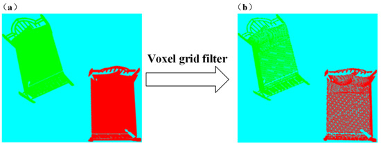
Figure 2.
Down sampling of the “Bed”; (a) the point cloud to be registered, (b) the down sampling result.
2.2. Intrinsic Shape Signatures Algorithm
Compared with Harris, Normal Aligned Radial Feature (NARF), and SIFT feature point extraction algorithms, the ISS is faster and the extracted feature points distribute more evenly. It has two main parts: a local reference frame (LRF) and a feature vector used to describe the points in the neighborhood around the basis point [16]. Figure 3 shows the schematic of ISS algorithm.

Figure 3.
Schematic of intrinsic shape signatures (ISS).
The steps of ISS algorithm are as follows:
Step 1, weighting the basis point. In order to establish the LRF of the basis point, the basis point and its adjacent points are weighted to compensate for uneven sampling of the point cloud, which can be described as
where is the weight of the , and is the radius of the sphere with as the center, which represents its weighted range.
Step 2, basis point eigenvalue analyzing. Do eigenvalue analysis at basis point with its neighbor points at a supporting radius . The covariance matrix can be calculated as
Step 3, LRF establishing. The eigenvalues and eigenvectors of were calculated and arranged in the order of decreasing magnitude. As shown in Figure 4, using as the origin, , and their cross product as the x, y, and z axes, the LRF can be established.
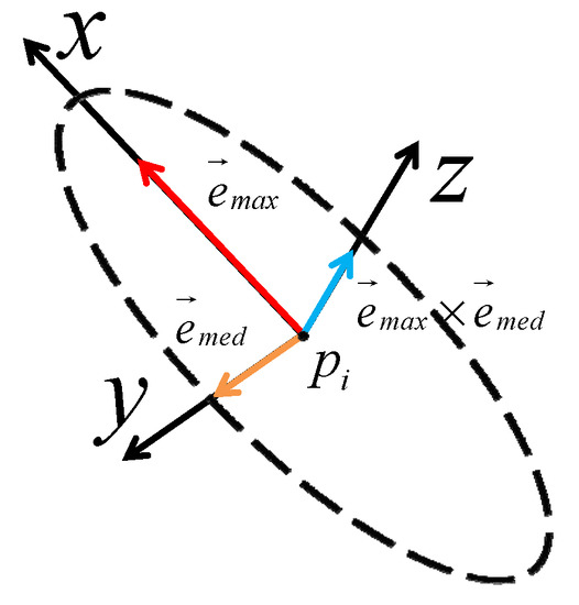
Figure 4.
Local reference frame (LRF) of basis point.
Step 4, feature points extracting. Set thresholds and , the points satisfying Equation (3) are regarded as ISS feature points. Figure 5 shows the feature points extracted by the ISS algorithm from the “Bed”.

Figure 5.
ISS feature points.
2.3. 3D Shape Context
The basic idea of 3DSC [17] feature descriptor is to count the context information of each point in two point sets and compare whether they are similar to obtain a most approximate arrangement, and find the corresponding points between the two point clouds. The feature space of 3DSC is shown in Figure 6.

Figure 6.
Three-dimensional shape context (3DSC) feature space division.
The description steps of 3DSC algorithm are as follows:
Step 1, normals calculating. For each query point in the point cloud, take as the center of the sphere, as the radius, and use the surface normal as the direction of North Pole to establish a local supporting area. Figure 7 shows the normals of the point cloud after down sampling.
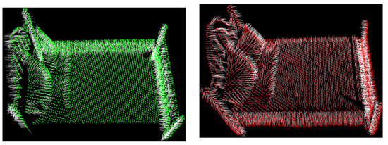
Figure 7.
The normals of the point cloud.
Step 2, sub-regions dividing and radiuses calculating. On the radius , divide J + 1 intervals by logarithm, divide L + 1 intervals along azimuth angle , and K + 1 intervals along pitch angle equally; thus sub-regions in total are divided. As the intervals are divided logarithmically on the radius, if the area near the sphere center is too small, it will be disturbed by noise easily. Setting as the minimum radius , and as the maximum radius , the radius is calculated by
Step 3, sub-regions weighting. Calculate the weights of each point in the area by Equation (5). Here represents the volume of the area for the j-th radius, the k-th azimuth direction, and the l-th elevation direction. is the density of the corresponding local point.
Step 4, feature vector composing. Then, make a statistic of the values of to compose a feature vector ,
where .This vector contains the shape context information around the basis point.
2.4. RANSAC Coarse Registration
The RANSAC algorithm proposed by Fischler and Bolles [18] can automatically fit the model in data, and the solution to the location determination problem shows that RANSAC can also calculate the position of the corresponding points, so it can be used for 3D point cloud registration. In our approach, we use an improved RANSAC algorithm [19] to calculate the initial transformation matrix , which minimizes the sum of the squared distances between the corresponding points of the two point clouds, as shown in Equation (7):
This algorithm needs to input the down-sampled source point cloud and target point cloud and the corresponding descriptors. The main steps are as follows:
Step 1, corresponding point searching. Select points randomly in for each iteration to find its corresponding point in by nearest neighbors matching of five feature descriptors.
Step 2, difference vector of corresponding sides calculating. Compute the Euclidean distance between the n sampling points at first. Then, calculate the ratio of the difference between the two corresponding side lengths to the bigger side length to form a vector . If is smaller than edge length similarity threshold , continue the next step, otherwise, return to the first step. Set n = 3 as a sample, is calculated as Equation (8) and the schematic diagram of computing is shown as Figure 8.
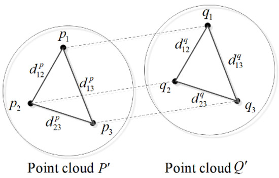
Figure 8.
The schematic diagram of computing .
Step 3, corresponding points transforming. Estimate a temporary transformation matrix from corresponding point pairs and transform into .
Step 4, inlier points judging. Compute the Euclidean distances of the nearest neighbors between and , and take the points whose nearest neighbor distance is lower than the set distance threshold as inlier points. If the number of inlier points is too small, go back to Step 1.
Step 5, transformation matrix computing. Compute the transformation matrix according to the corresponding relationship of the interior points. The iteration number k of RANSAC is obtained by a presumed success probability p and a preset inlier fraction w, which is shown as Equation (9):
Step 6, model estimating and updating. Use the inlier points fitting a parameterized model to test other points, and update the inlier points to continue iterative calculations until the best estimation model is obtained or max iteration number is reached. When the value of is the smallest, set as the best estimation result and stop the iteration.
2.5. ICP Fine Registration
When the ICP algorithm registers the two point clouds P and Q, it searches for the nearest neighbor point pairs that meet certain constraints, and calculates the optimal rotation matrix and translation matrix to minimize the error function. The larger the amount of data in the point cloud, the more time-consuming it is to query the point pairs. In our approach, we use the KD tree in the ICP algorithm, which can quickly search for neighbor point pairs and improve the registration efficiency [20]. The specific process of registration is as follows:
Step 1, nearest neighbor points searching. Use the KD tree algorithm to search for the nearest neighbor of the point () in Q, and minimize the Euclidean distance .
Step 2, optimal rotation matrix and rotation matrix solving. Use the least square method to solve the optimal rotation matrix R and translation matrix T, the error function G(R, T) is minimized.
Step 3, source point cloud transforming. Perform R, T transformation on the point cloud P, and get the transformed corresponding points , then calculate the average distance of point pair :
Step 4, threshold judging. Set the threshold , if the conditions are met, end the iteration, otherwise iterate goes on.
Step 5, registration completing. According to the finally obtained R and T, the point cloud P is transformed into the coordinate system of the point cloud Q to complete the registration.
3. Experimental Results
The experiment dataset contains “Bed”, “Motorbike”, and “Piano” from the basic geometry library and “Dragon1”, “Dragon2”, and “Bunny” from Stanford University Graphics Lab. The point numbers of the point clouds are Bed (110372, 108615), Motorbike (41214, 40023), and Piano (54139, 54139), Dragon1 (126546, 132000), Dragon2 (184982, 155208), Bunny (40256, 40097). Our proposed algorithm is implemented in Microsoft Visual Studio 2015 and PCL (Point Cloud Library), while all the experiments are conducted on a 3.6 GHz Intel(R) Pentium(R) G4600 processor with 8 GB RAM. In order to verify the rationality and efficiency of the algorithm in this paper, it is compared with ICP, and sample consensus initial alignment ICP (SAC-IA+ICP), and 3D histograms of point distributions ICP (3DHoPD+ICP) [21] algorithms under the same environment.
3.1. Selection of Main Parameters
The algorithm in this paper changes the registration result by modifying the parameters. Through the registration error returned by the experimental results, we find that many parameters are related to the grid size of the point cloud. Root mean square error (RMSE) is the error measurement method often used in point cloud registration, which means the average of the sum of squared distances between the corresponding points of two point clouds. It is defined as
where, and are nearest neighbors in pair, located in data P and Q, respectively, and N and M represent the registration scales of P and Q. The smaller the RMSE, the better the registration result.
Table 1 shows the number of sampling points and ISS feature points under different grid sizes, the first two lines belong to source point cloud P, the rest belongs to Q. In order to reduce the running time of the algorithm, the number of sampling points is generally several thousand. Considering that too many feature points will increase the calculation time, and too few will affect the registration accuracy, the grid size is selected as 0.03 m.

Table 1.
The number of sampling points and feature points under different grid sizes.
For the 3DSC algorithm, the main parameters are , , and . denotes the support radius for 3DSC and is usually set to 10 times of the grid size. is the minimal radius value for the search sphere, which is often set same scale with the grid size. is the density of the corresponding local point, which is set one-tenth of .
Table 2 shows the registration results of different , when the initial value of is 0.1 m. When = 0.3 m, the registration time is the least and the RMSE is also the smallest.
Table 2.
= 0.1 m, the registration results of different .
Table 3 shows the registration results of different , when = 0.3 m. When = 0.3 m, the RMSE is the smallest.
Table 3.
= 0.3 m, the registration results of different .
Figure 9 shows the registration results of “Bed” with different grid sizes. It can be seen from the figure that as the grid size increases, the registration time and the number of ISS-3DSC features continue to decrease, and the RMSE value is quite small in the range of 0.02 m to 0.04 m, so we set the grid size to be 0.03 m. More parameters are listed in Table 4.

Figure 9.
The result of registration under different leaf sizes.
Table 4.
Parameters set of this algorithm.
3.2. Evaluation
RMSE can roughly represent the registration result, but it is not accurate enough. The point clouds to be registered are often not complete models, some points have no corresponding points, so the calculated RMSE may not be suitable. Additionally, when debugging the parameters, only from the RMSE results, it is not known how many points in the point cloud are involved in the registration [22]. We improved RMSE to better describe the registration results of the incomplete models, and named it the effective root mean square error (ERMSE). We set parameters and . is the distance threshold. If the calculated Euclidean distance of the nearest neighbor pair is less than , it is judged as a corresponding point, otherwise, it is a non-corresponding point. is the ratio of the number of the corresponding points involved in the registration to that of the point cloud. The expressions of and ERMSE are shown in Equation (13).
where k represents the number of non-corresponding points, N represents the number of points in the registered point cloud, and N−k represents the number of corresponding points, and represent the nearest neighbor pair in the two point clouds.
As shown in Figure 10, we used ICP, SAC-IA+ICP, 3DHoPD+ICP and our approach for the registration of Bed, Motorbike, Piano, Dragon1, Dragon2, and Bunny point clouds. For the Bed, Motorbike, Piano, and Dragon1 models with large initial pose deviations, the registration rate of the ICP algorithm is 0, and the ERMSEs are meaningless. However, its registration accuracies for Dragon2 and Bunny are quite high, which just reflects the advantages of ICP for small initial pose deviations. The SAC-IA+ICP algorithm, 3DHoPD+ICP algorithm, and our proposed algorithm have almost the same registration rate for the six models with the increase of , and when , the registration rates are all over 90%. However, the registration accuracy of our approach is higher for models with large initial pose deviations. From the experimental results of Dragon2 and Bunny, we can see that for models with small initial pose deviations, the registration accuracies of ICP, SAC-IA+ICP, and our method algorithms are almost the same, while 3DHoPD+ICP algorithm is higher than them. From Figure 10, we can also get that with the increase of , the values of and ERMSE also increase gradually. This is because the point cloud is not completely matched, and the greater the distance threshold, the greater the error. Therefore, needs to be limited.
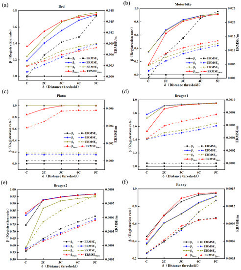
Figure 10.
Analysis of registration resultsby iterative closest point (ICP), sample consensus initial alignment (SAC-IA+ICP), 3D histograms of point distributions ICP (3DHoPD+ICP) and our method. (a) Bed, (b) Motorbike, (c) Piano, (d) Dragon1, (e) Dragon2, (f) Bunny.
Through the above experiments and the determination of the ERMSE values, we compared the magnitude of RMSEs and ERMSEs for the four methods as shown in Figure 11. Here, ICP uses the right vertical coordinate and SAC-IA+ICP, 3DHoPD+ICP, and our method use the left vertical coordinate. Figure 11 shows that the ERMSE error is slightly lower than RMSE, and agree with the change trend of RMSE.
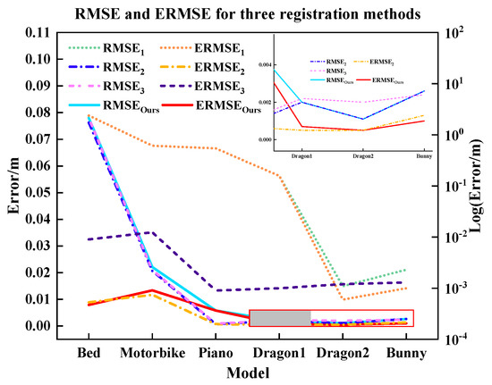
Figure 11.
Root mean square error (RMSE) and effective root mean square error (ERMSE) of ICP, SAC-IA+ICP, 3DHoPD+ICP, and our method.
Table 5 shows the final RMSE, , and ERMSE values of ICP, SAC-IA+ICP, 3DHoPD+ICP, and our method for the six models, and the best results are highlighted in bold font. From the experiment results, we can see that ICP cannot be used for models with large initial pose deviations, while SAC-IA+ICP, 3DHoPD+ICP, and our method can be used for all the models, and their registration accuracies are both quite high.
Table 5.
RMSE, , and ERMSE of ICP, SAC-IA+ICP, 3DHoPD+ICP, and our method for the six models.
Table 6 shows the registration time of each algorithm for the six models in the conditions. We can see that our approach is the most efficient. The total registration time of our method for the six models is only about 1/25 of SAC-IA+ICP method and 1/2 of 3DHoPD+ICP method. To get the reason of the performance in details, we compared the operating time of ICP registering, and before this step, between 3DHoPD+ICP method and ours. For the model of Bunny, the ICP registering time of our method is four orders of magnitude lower than that of the 3DHoPD+ICP method, while the preparing time is about 0.4 s higher than it. This result indicates that for the entire point clouds registration process, optimizing feature descriptors is a more effective way.
Table 6.
Registration time for six models of each algorithm/s.
The registration results of each algorithm are shown in Figure 12. In the experiments, the source point clouds are in green, the target point clouds are in red, and the registered point clouds are in blue. It can be seen from the results that the ICP has a large registration error for the point cloud with large initial positions, and the registration of Bed, Motorbike, Piano, and Dragon1 point are failed. The SAC-IA-IA+ICP algorithm, the 3DHoPD+ICP algorithm, and our method have nearly the same registration results for the six models, which are all registered successfully. On the other hand, our approach has the least registering time, showing a higher efficiency. Hence, this algorithm has a significant improvement over others.
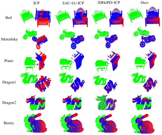
Figure 12.
Registration results of each algorithm.
4. Discussion
In the process of point clouds registration, descriptors can often determine the final performance. There are many different approaches, but all of them have the same target: providing a useful representation of the shape around the given point that facilitates searching for correspondences between two shapes, thereby avoiding exhaustive searches. Combining a good descriptor with a sophisticated searching strategy would improve the efficiency of the methods. In this article, we proposed a fast point cloud registration algorithm based on ISS-3DSC feature descriptors, an improved RANSAC algorithm and ICP algorithm. The RANSAC algorithm can estimate high-precision parameters from a large number of data sets. Its disadvantage is that the number of iterations for different models is significantly different and there is a certain probability of getting wrong results, which need to be improved by subsequent fine registration. Different from the classic RANSAC algorithm, the improved RANSAC algorithm uses both surface and feature descriptors to describe a point. Wrong assumptions are removed in time, and the time for a lot of pose assumptions is reduced. This method has too many parameters to be set artificially, which is not conducive for intelligent registration; in the next step, we will develop a new framework to solve this problem.
5. Conclusions
We proposed a fast point cloud registration algorithm based on ISS-3DSC feature descriptors. By comparing with ICP, SAC-IA+ICP, and 3DHoPD+ICP algorithms on different point cloud samples, we have shown that this algorithm has a good registration accuracy, and it is more efficient than the others. The registration time is less than 1 second for all of the models, while the registration errors are only 0.01% or less. We have also proposed an evaluating parameter ERMSE on the basis of RMSE, and prove through the experiments that ERMSE is better than RMSE to describe the point cloud registration error. When working with real data perturbed by noise and occlusions and related to real-life applications, a large number of points are often necessary, and thus efficiency becomes a key factor. The 3D representation would benefit from non-subsampled point clouds in order not to lose any data, or to minimize data loss. Future work should also address working with optimized real-world point clouds, understanding this optimization as the process of removing noise and subsampling to its minimum expression.
Author Contributions
Conceptualization, G.X. and Y.P.; methodology, Z.B.; software, G.X.; validation, G.X., Y.P., and Z.B.; formal analysis, Y.W.; investigation, G.X. and Y.P.; resources, Y.W. and Z.L.; data curation, G.X.; writing—original draft preparation, G.X.; writing—review and editing, Y.P.; visualization, G.X.; funding acquisition, Z.L. and Y.P. All authors have read and agreed to the published version of the manuscript.
Funding
This research was funded by the National Natural Science Foundation of China (grant number 61927815, 61905063, and 61905061); the Hebei Science and Technology Innovation Strategy Funding Project (no. 20180601); the Natural Science Foundation of Hebei Province, China (grant number F2020202055).
Institutional Review Board Statement
Not applicable.
Informed Consent Statement
Not applicable.
Data Availability Statement
Not applicable.
Conflicts of Interest
The authors declare no conflict of interest.
References
- Besl, P.J.; McKay, N.D. A method for registration of 3-D shapes. IEEE Trans. Pattern Anal. Mach. Intell. 1992, 14, 239–256. [Google Scholar] [CrossRef]
- Hong, S.; Ko, H.; Kim, J. VICP: Velocity updating iterative closest point algorithm. In Proceedings of the 2010 IEEE International Conference on Robotics and Automation, Anchorage, AK, USA, 3–7 May 2010; pp. 1893–1898. [Google Scholar]
- Segal, A.; Haehnel, D.; Thrun, S. Generalized-ICP. In Robotics: Science and Systems V; University of Washington: Seattle, DC, USA, 2009; Volume 2, p. 435. [Google Scholar]
- Yang, J.; Li, H.; Jia, Y. Go-ICP: Solving 3D registration efficiently and globally optimally. In Proceedings of the 2013 IEEE International Conference on Computer Vision, Sydney, Australia, 1–8 December 2013; pp. 1457–1464. [Google Scholar]
- Censi, A. An ICP variant using a point-to-line metric. In Proceedings of the 2008 IEEE International Conference on Robotics and Automation, Pasadena, CA, USA, 19–23 May 2008; pp. 19–25. [Google Scholar]
- Magnusson, M.; Lilienthal, A.J.; Duckett, T. Scan registration for autonomous mining vehicles using 3D-NDT. J. Field Robot. 2007, 24, 803–827. [Google Scholar] [CrossRef]
- Chang, S.; Ahn, C.; Lee, M.; Oh, S. Graph-matching-based correspondence search for nonrigid point cloud registration. Comput. Vis. Image Underst. 2020, 192, 102899. [Google Scholar] [CrossRef]
- Shui, W.; Zhou, M. An approach for model reconstruction based on multi-view scans registration. In Proceedings of the 2010 International Conference on Audio, Language and Image Processing, Shanghai, China, 23–25 November 2010; pp. 601–606. [Google Scholar]
- Li, J.; Qian, F.; Chen, X. Point cloud registration algorithm based on overlapping region extraction. J. Phys. Conf. Ser. 2020, 1634, 012012. [Google Scholar] [CrossRef]
- Mohamad, M.; Ahmed, M.T.; Rappaport, D.; Greenspan, M. Super generalized 4PCS for 3D registration. In Proceedings of the 2015 International Conference on 3D Vision, Lyon, France, 19–22 October 2015; pp. 598–606. [Google Scholar]
- He, Y.; Lee, C.-H. An improved ICP registration algorithm by combining PointNet++ and ICP algorithm. In Proceedings of the 2020 6th International Conference on Control, Automation and Robotics (ICCAR), Singapore, 20–23 April 2020; pp. 741–745. [Google Scholar]
- Kamencay, P.; Sinko, M.; Hudec, R.; Benco, M.; Radil, R. Improved feature point algorithm for 3D point cloud registration. In Proceedings of the 2019 42nd International Conference on Telecommunications and Signal Processing (TSP), Budapest, Hungary, 1–3 July 2019; pp. 517–520. [Google Scholar]
- Xiong, F.; Dong, B.; Huo, W.; Pang, M.; Kuang, L.; Han, X. A local feature descriptor based on rotational volume for pairwise registration of point clouds. IEEE Access 2020, 8, 100120–100134. [Google Scholar]
- Chen, L.C.; Hoang, D.C.; Lin, H.I.; Nguyen, T.H. Innovative methodology for multi-view point cloud registration in robotic 3D object scanning and reconstruction. Appl. Sci. 2016, 6, 132. [Google Scholar] [CrossRef]
- Bueno, M.; González-Jorge, H.; Martínez-Sánchez, J.; Lorenzo, H. Automatic point cloud coarse registration using geometric keypoint descriptors for indoor scenes. Autom. Constr. 2017, 81, 134–148. [Google Scholar] [CrossRef]
- Zhong, Y. Intrinsic shape signatures: A shape descriptor for 3D object recognition. In Proceedings of the 2009 IEEE 12th International Conference on Computer Vision Workshops, ICCV Workshops, Kyoto, Japan, 27 September–4 October 2009; pp. 689–696. [Google Scholar]
- Frome, A.; Huber, D.; Kolluri, R.; Bülow, T.; Malik, J. Recognizing objects in range data using regional point descriptors. In European Conference on Computer Vision; Springer: Berlin/Heidelberg, Germany, 2004. [Google Scholar]
- Fischler, M.A.; Bolles, R.C. Random sample consensus: A paradigm for model fitting with applications to image analysis and automated cartography. Read. Comput. Vis. 1987, 24, 726–740. [Google Scholar] [CrossRef]
- Buch, A.G.; Kraft, D.; Kämäräinen, J.-K.; Petersen, H.G.; Krüger, N. Pose estimation using local structure-specific shape and appearance context. In Proceedings of the 2013 IEEE International Conference on Robotics and Automation, Karlsruhe, Germany, 6–10 May 2013; pp. 2080–2087. [Google Scholar]
- Li, S.; Wang, J.; Liang, Z.; Su, L. Tree point clouds registration using an improved ICP algorithm based on kd-tree. In Proceedings of the 2016 IEEE International Geoscience and Remote Sensing Symposium (IGARSS), Beijing, China, 10–15 July 2016; pp. 4545–4548. [Google Scholar]
- Prakhya, S.M.; Lin, J.; Chandrasekhar, V.; Lin, W.; Liu, B. 3DHoPD: A fast low-dimensional 3-D descriptor. IEEE Robot. Autom. Lett. 2017, 2, 1472–1479. [Google Scholar] [CrossRef]
- Li, C.L.; Dian, S.Y. Dynamic differential evolution algorithm applied in point cloud registration. IOP Conf. Ser. Mater. Sci. Eng. 2018, 428, 012032. [Google Scholar] [CrossRef]
Publisher’s Note: MDPI stays neutral with regard to jurisdictional claims in published maps and institutional affiliations. |
© 2021 by the authors. Licensee MDPI, Basel, Switzerland. This article is an open access article distributed under the terms and conditions of the Creative Commons Attribution (CC BY) license (https://creativecommons.org/licenses/by/4.0/).