
An Efficient Semi-Analytical Scheme for Determining the Reflection of Lamb Waves in a Semi-Infinite Elastic Waveguide

1
Department of Mathematics, The University of Manchester, Manchester M13 9PL, UK
2
Department of Applied Mathematics and Theoretical Physics, University of Cambridge, Cambridge CB3 0WA, UK
*
Author to whom correspondence should be addressed.
Appl. Sci. 2022, 12(13), 6468; https://doi.org/10.3390/app12136468
Submission received: 14 April 2022
/
Revised: 21 June 2022
/
Accepted: 22 June 2022
/
Published: 25 June 2022
(This article belongs to the Special Issue Ultrasonic Modelling for Non-destructive Testing)
Abstract
:The classical problem of reflection of Lamb waves from a free edge perpendicular to the centre line of an elastodynamic plate is studied. It is known that Lamb wave expansions for the displacement and stress fields poorly represent the irregular behaviour near corners, leading to the slow convergence of a series of such waves. The form of the irregularity for an elastodynamic corner is derived asymptotically, and a new solution method, which incorporates this corner behaviour analytically, is then implemented. Results are presented showing that this new approach represents the near-field and far-field behaviour very accurately, requiring very modest numbers of Lamb wave and corner modes. Further, it is revealed that the method can recover the trapped-mode phenomenon encountered in this configuration at the Lamé frequency and a specific Poisson’s ratio that we find to be approximately .
1. Introduction
We are interested in the use of guided wave techniques in non-destructive testing, applied specifically to the problem of hidden tamper detection in an arms control context. In arms control it is essential to ensure that all parties are in compliance with the terms of a treaty. A problem arising from this necessity is tamper detection [1]. The competent authorities wish to ensure that items of interest cannot be accessed for long periods of time and to this end they are sealed in freight-like containers. However, with sufficient time and effort any container can be breached, hence we will focus on the problem of making these containers ‘tamper indicating’. This means that if a container is breached, it should be impossible to hide the evidence of this from a verification process, even if the breach has been deliberately concealed. Such a deliberately concealed breach is known as a ‘hidden tamper’.
We wish to apply a well known, non-destructive testing method to tamper detection, i.e., that of guided elastic waves. This has been motivated by experimental evidence [2] that tampers can be detected easily, even by non-specialist technicians, by scanning for mode conversion of elastic waves. Refraction and reflection of the guided wave, or excitation of additional modes, may occur due to welds [3], cracks [4], or other inhomogenous imperfections at the boundary of the tamper; however, we are mainly interested in mode conversion due to asymmetry introduced by the tamper itself.
In elastic plates, there are two types of modes that propagate, symmetric and antisymmetric, and these modes travel at different speeds. For a plate of given thickness and material properties, the number of cut on (i.e., propagating) symmetric and antisymmetric modes depends on the frequency, with the lowest antisymmetric mode, , moving more slowly than its symmetric counterpart, . When elastic waves are initially generated from a known source location, the region where the slower modes are present at any given time is bounded. Any slower modes found outside this region must therefore be caused by mode conversion from the faster waves interacting with a hidden tamper. Due to the symmetric and antisymmetric nature of the two types of modes, converting between the two requires some asymmetry around the mid-plane of the plate. An example of how a tamper could introduce asymmetry is as follows: a section of the container could be removed to gain internal access, and later replaced by a plate of slightly greater thickness; it could then be polished flat on the outside wall to hide it from detection. However, it cannot be polished on the inside wall as the container is sealed, hence there will exist an indentation or protrusion on the inaccessible inner side; this feature is asymmetric and induces mode conversion. A schematic diagram of such a hidden tamper is given in Figure 1, which shows that the tamper is asymmetric about the mid-plane.
It has been shown [5] that the stress field near traction-free elastic corners with an internal angle greater than are locally singular; in Figure 1, two such corners are present. This leads us to believe that the corners could have a large effect on the solution of the problem and their asymmetric positioning about the mid-plane implies that this effect will include mode conversion. The local stress fields near a traction-free corner of internal angle less than are not singular, but are irregular. This means that they are bounded in the vicinity of the corner, but behave locally as a non-integer power of the distance from the corner. For sufficiently low frequencies, the wavelengths of the propagating modes are much longer than the corner lengthscales, therefore the local behaviour around the corner is unimportant away from it; however, even in such low-frequency regimes, the behaviour near sharp corners strongly affects the accuracy of methods for determining the global solution [6]; we shall see that this is true even for irregular, but non-singular, corner behaviour.
In this article, as a first step towards the tamper model, and as a useful way to demonstrate the novel solution method, we examine a simpler problem that incorporates corner behaviour. We will consider the reflection of an incoming time-harmonic, symmetric wave in a semi-infinite elastic waveguide, as shown in Figure 2. In this problem we have symmetry about the mid-plane and hence no asymmetric mode conversion; however, it will allow us to study how sharp corners affect the reflection problem. The corners in this problem each have an internal angle less than , which means that the stress field around them is bounded. This problem may be solved by traditional methods, such as spectral collocation [7], allowing us to generate solutions to compare against; hence, this is a good test case to implement and validate our new method to deal with irregular corner behaviour. In addition to this goal, this canonical problem is also associated with the important question of the existence of a trapped mode, which in this case occurs at the Lamé frequency and at a particular value of Poisson’s ratio, which we will discuss in Section 3.2 [7,8,9].
We wish to find the solution to this problem in terms of the in-plane natural modes of elastic waveguides, as these are the waves that are of experimental interest. These were first studied by Lamb over one hundred years ago [10] and are still an active area of research due to their very wide range of applications in areas such as nondestructive testing, seismology, and vibration control. The two sets of modes (in this article, we may ignore the third set of modes, the out-of-plane polarized shear waves, which are decoupled from the other two in the problem of interest) are the faster symmetric and the slower anti-symmetric modes, the wavenumbers of which satify different dispersion relations. Finding the roots of these relations is non-trivial, but methods relying on finite-product formulae [11], asympototic analysis, or projection onto Chebyshev polynomials [7] can be used efficiently to this end. The solutions to each dispersion relation consist of a single propagating mode that always exists (the or mode), a finite number of higher propagating modes that cut on depending on frequency, and an infinite number of evanescent modes.
It has been known for some time [6,12] that the solution to the present canonical problem in terms of a modal expansion of Lamb waves is slowly convergent near the free end, and poorly represents the behaviour of the field near the corners. This is essentially due to the Gibbs phenomenon. There are a variety of numerical treatments that can be applied in this and other waveguide problems to aid convergence, including the Lanczos -approximation (see, e.g., [13,14]).
Note that difficulties arising from geometric singularities in waveguides when using a naive modal expansion do not only occur in the elastodynamic case considered presently. In fact, the corner mode expansion method presented in this paper was first conceived in the context of easier, scalar, acoustic problems [15]. Moreover, other authors have considered such problems in, for instance, acoustic waves [16,17], water waves [18,19], horizontal shear waves [20], and electromagnetic waves [21,22]. Most of these methods take an ingenious numerical approach relying on the use of an expansion in terms of a carefully chosen family of orthogonal polynomials (Chebyshev, Gegenbauer, Jacobi, etc.), which can effectively be used to tackle certain corner singularities and ‘fix’ the naive modal expansions.
In the present work, rather than trying (in vain) to find known special functions with the required singular behaviour, we let them emerge naturally from the physical problem, giving rise to what we call the corner modes. This method has the advantage of not requiring an a priori knowledge of the singularities at hand and can accommodate rather complicated singular behaviours.
As hinted above, the aim of this paper is to apply a new approach tailored to the specific physical nature of the irregularity. We will introduce new modes that accurately represent the irregular behaviour near the corners and add them to the Lamb wave terms, which well represent the smooth part of the field elsewhere. This paper offers an application of the new method in the context of elastodynamics, whilst contemporaneous applications are presented in [15], for acoustic problems, and [23], for a model problem in elastostatics. However, the present work also requires an interesting additional step. That is, it is convenient for mathematical purposes to imagine that the plate shown in Figure 2 is infinite in extent, and has specified traction boundary forcing on the top and bottom faces in to ensure that the prescribed boundary conditions on are satisfied (i.e., that the total normal and shear stresses on are zero.) This geometry is illustrated in Figure 3, noting that the extension of the plate is a purely virtual construct; however, from Green’s theorem, it can easily be shown that there will always exist forcing functions, that ensure the correct boundary conditions on the actual plate edge, .
The remainder of this paper is organised as follows. In Section 2.1, we recast the problem as an infinite plate, with (as yet unknown) boundary tractions on the faces of the semi-infinite virtual extension of the plate. We then write the solution to this new problem in Fourier space. In Section 2.2, we find an asymptotic representation of the new unknown boundary conditions in terms of the behaviour associated with the corners. Next, we summarise the known similarity solutions of the stress field associated with a static elastic corner before going on to implement an asymptotic technique to recover the similarity solutions for the stresses in an elastodynamic corner. In Section 2.3, we discuss how the corner behaviour, as determined in Section 2.2, can be expressed as a sum of corner modes. These new corner modes will enable us to write the field as an expansion of the form
In this representation, the Lamb modes capture well the far field behaviour, which is of interest experimentally, while the corner modes accurately describe the near field behaviour, which is important when applying the edge boundary conditions to determine the reflection coefficients. We then highlight the excellent convergence properties of such an expansion in Section 3. We present some results obtained by including both corner and Lamb modes, and illustrate the superiority of our method (compared to the pure Lamb mode expansion) when it comes to the reconstruction of the stresses on the free end of the plate and the prediction of the propagating waves reflection coefficients. We conclude by showing that our new method can predict the trapped-mode appearing at the Lamé frequency and find the specific value of the Poisson ratio at which it occurs as approximately .
2. Materials and Methods
2.1. A Useful ‘Equivalent’ Problem: A Forced Infinite Elastic Plate
Virtual Plates
As mentioned above, we know from Green’s theorem that the problem shown in Figure 3, with certain prescribed tractions , , , and , is equivalent, in , to the posed semi-infinite free-end model.
We have introduced this auxiliary problem because it has two useful properties that the original problem does not possess. First, it easily admits solutions in terms of the unknown tractions by way of Fourier transform, as we will demonstrate. Second, by approximating the prescribed tractions, it will allow us to find a convenient way of inputting the desired near-corner behaviour into a modal expansion.
The first step is to solve the equivalent problem in terms of the prescribed tractions. We begin with the time-harmonic (angular frequency ) potential forms of the Navier–Lamé equations, and we non-dimensionalize spatial variables using the thickness of the plate, h, as a suitable lengthscale. The dimensionless potentials and are related to the dimensionless displacement in the x-direction, u, and in the y-direction, v, by
the dimensionless potentials are governed by the Helmholtz equations
where and are, respectively, the dimensionless free space longitudinal and transverse wavenumbers for the material, given in terms of the plate density and the Lamé constants and , as and . One of these wavenumbers, along with Poisson’s ratio , say, may be used to fully define our elastic material for a given frequency and plate thickness. However, it is slightly more convenient to introduce the constant K as the ratio of the transverse wavenumber to the longitudinal wavenumber, so that The stresses are then related to the potentials in the usual way by
We seek solutions to the boundary value problem shown in Figure 3 by use of a Fourier transform defined by
where is the spectral variable. The Fourier transformed Helmholtz equations are given by
where the capital letters and are the Fourier transforms of and , respectively. The general solutions to these equations are given by
where we have defined
the stresses in Fourier space are denoted by and are given by
the Fourier transformed boundary conditions are , , , and , where
etc., and the superscript ‘+’ (‘−’) notation denotes a ‘plus’ (‘minus’) function, that is, a function that is analytic in the upper (lower) half of the complex -plane. Note that, from the theory of half-range Fourier transforms [24], we know that such well-behaved functions are analytic in the upper or lower half space of the -plane.
We may use the symmetry of the general solutions to simplify the boundary conditions. Using the linear combination of boundary conditions given by and , we find that the unknown coefficients A and D can be found by solving a system decoupled from the system governing B and C. The solutions for A and D are known as the symmetric part and must satisfy the linear system given by
for the antisymmetric part, we use the combination of conditions given by and . This generates the linear system given by
In linear theory, the symmetric and antisymmetric solutions do not interact at a symmetric boundary. Therefore, if we assume a symmetric incoming wave, the contributions from the antisymmetric Lamb waves must be zero. This implies that and Similarly for the antisymmetric case, the symmetric waves must be zero, which requires and
We will present the method for symmetric waves here; the antisymmetric case follows similarly. By taking the inverse of the first matrix in (17), we find that A and D are functions of given by
where
is the determinant of the matrix to be inverted in (17). The relation is known as the dispersion relation for symmetric Lamb waves. We may now use the expressions for A and D to find the transformed potentials and stresses. The symmetric part of the transformed potentials are given by
From the potentials, we find the transformed stresses to be
where , , , , and are analytic functions given by (21),
The solution for the Potentials (22) and (23), or stresses (24) and (25), fully describes the problem in terms of the Fourier transforms of the unknown functions s, p, q, and r. Whilst we do not know these functions exactly, we can approximate them from knowledge of their behaviour near a corner, which we will examine in Section 2.2.
2.2. Similarity Solutions in the Corner of an Elastic Body
We now seek to establish the form of the unknown boundary conditions on the virtual extension of the plate. To do this, let us consider the physical problem local to a corner of an elastic wedge. We know that, near a corner, these conditions will be formed of regular contributions from the Lamb waves and irregular contributions from the similarity solutions associated with this corner. As the Lamb waves have zero traction on the virtual boundaries, the conditions will be dominated by the similarity solutions, the derivation of which will be the subject of this section. In doing so, we will directly obtain the behaviour that the Lamb wave representation has trouble capturing.
The corners in this model problem both have the same internal angle, ; however, there is little extra complexity in presenting the solutions for arbitrary internal angle; hence this is what will be presented here. Figure 4 shows an infinite arbitrary-angled traction-free corner. We consider the two traction-free edges to meet at an angle (where is the interior angle). We introduce a planar polar coordinate system with at the corner and with the line as the bisector of the angle . Choosing the bisector as the coordinate curve allows us to consider two families of solutions (symmetric and antisymmetric in ) separately, which simplifies the algebra. The normal vector to each edge lies in the direction, therefore the traction-free conditions are and .
2.2.1. Elastostatic Expansion
It has been known for over 50 years that static deformations (eigensolutions) in a two-dimensional corner of an elastic material can be found by use of an Airy stress function, an approach that is well understood for similar problems (see, e.g., [25]). We shall examine this briefly here, and then move on to the more-relevant elastodynamic case afterwards. Following [5], we pose an Airy stress function of the form where , from which we can recover the stresses as
Then, Navier’s equation is satisfied, and compatibility yields , which requires that the dependence is of the form
We now apply the boundary conditions, and use the symmetry properties of the dependence as given in (31) to simplify the problem. We do this by considering the linear combinations of conditions given by and , which yield two decoupled linear systems of equations given by
In order for these conditions to possess non-trivial solutions to the homogeneous problem, the determinants must be equal to zero, which yields constraints on the corner exponents:
In (34), a positive sign corresponds to the determinant of the first system (32) and an Airy stress function symmetric around , while the negative sign corresponds to the determinant of the second system (33) and an Airy stress function antisymmetric about . In order for the solutions to be physical, we must also have finite displacements, which limits the solutions to those where .
The roots of (34), which can easily be found numerically, are labelled and ordered according to the size of the real parts, and also by imaginary parts when two roots have the same real part. For each solution of the compatibility condition (34) we find a non-trivial solution to the homogeneous problem with a single unknown constant; we can therefore write a general similarity solution as the series
for arbitrary number of terms M. Here and are known functions and are arbitrary unknown constants, each associated with the mth similarity solution.
2.2.2. Elastodynamic Expansion
We now wish to consider the local problem relevant to this study, i.e., the local dynamic (irregular) behaviour in the vicinity of a corner of the form shown in Figure 4. That is, we want to find (eigen-)solutions to the dynamic Navier-Lamé equation in this corner domain with traction-free boundary conditions. We begin by noting that in the limit where the distance to the corner becomes small, , the dynamic terms become small. This implies that the leading-order contributions in the elastodynamic case should correspond to the similarity solutions obtained in the static case.
In this section, we will show that for any given , the asymptotic expansions of the elastodynamic stresses and as are given by
where is the largest positive integer m such that , and
where is the largest integer ℓ such that and the functions and are known exactly. Hence, the only unknowns in the expansions (37) are the coefficients . Note that for this expansion to be formally correct, we need to choose a that is not equal to the real part of any of the static roots .
In order to justify this expansion, we again use the Helmholtz decomposition, but this time non-dimensionalised on the longitudinal dimensional wavenumber, , as there is no natural lengthscale for an infinite wedge. We again write the displacements in terms of potentials, as in (1) and (2), but here the Navier–Lamé equations reduce to
where, as before, .
Using separation of variables, we find that the non-dimensional potentials and corresponding to a given static root , which solve (39), are given by
where, for convenience, we have introduced the reduced index
and is the Bessel function of the first kind of order . The unknown coefficients , , , and will be determined by imposing traction-free boundary conditions.
The normal and shear stresses in polar coordinates, and , may now be written in terms of these potentials as
and traction-free conditions for the corner under consideration are . It is convenient to rewrite these conditions as
Note that the conditions (43) only involve the unknowns and , while the conditions (44) only involve the unknowns and .
Let us now, for brevity, consider a root that is associated with a symmetric Airy stress functions, i.e., a root of (34) with the + sign. The case of an anti-symmetric root can be dealt with similarly. It will be helpful to introduce the quantity , defined for by
Rewriting the Bessel functions as series expansions about , and collecting the terms of order in (43) (to do so, one only needs to consider the terms with in (40) and (41)), we obtain
implying that , and giving an explicit link between and . Note that this implies that, as expected from the static case, our expansion does not actually have any terms of order .
Using the relationship , and collecting this time the terms of order in (43) (to do so, one only needs to consider the terms with and 1 in (40) and (41)), we obtain
This is a linear system of two equations for the two unknowns and , whose associated determinant can be shown to be , which is known to be equal to zero given our choice of . Hence, this system admits non trivial solutions that take the form of an explicit expression for in terms of . Note that we recover here the static behaviour of Section 2.2.1.
Let us now collect the terms of order in (43) (to do so, one only needs to consider the terms with and 2 in (40) and (41)). This leads to two independent linear equations for the three unknowns , and . This system is always solvable in terms of the single constant .
The process of increasing the order is now algorithmic. In a consistent expansion of the stresses up to and including the order for , all the unknown coefficients , and are known exactly in terms of a single unknown constant . If we now follow exactly the same process, but for the boundary conditions (44), we will find that the coefficients and are all equal to zero. Hence, whatever the asymptotic order we want to reach (determined by a choice of ), the consistent expansion obtained for the potentials corresponding to each static root only involves a single unknown coefficient. This is why we can reconstruct the stresses as in (37) and (38), where the and functions are known exactly. The exact form of these functions is found by an automatic implementation of the asymptotic procedure described above, which was implemented by the authors using the mathematical software package Mathematica.
2.3. Expressing the Virtual Forcing in Terms of Corner Modes
In Section 2.1, we found a Fourier-space solution in terms of functions describing the stress fields on the surfaces of the virtual extension to the plate. These functions can now be expressed in terms of the similarity solutions found in Section 2.2. Further, in this section we will use this information to introduce new modes that will prove extremely helpful in efficiently solving the present boundary value problem illustrated in Figure 2.
2.3.1. Inverse Transformation of the Forced Plate
We can now approximate the unknown functions from Section 2.1, s, p, q, and r, as a series of the similarity solutions associated with a corner of angle , found in Section 2.2, which we can extend mathematically beyond the physical corner. We use polar coordinates consistent with that defined in Figure 4, i.e., angles are measured from the respective corner bisectors as shown in Figure 5. Hence, the virtual upper boundary is defined by , whereas corresponds to the virtual lower boundary on the lines , , and , so we can express the forcing terms in Cartesian form, which yield approximations, correct up to order , as
The solutions in Section 2.1 were found in terms of the Fourier transform of these virtual conditions, which we write as
where the transforms can be determined analytically.
Combining the transforms of the virtual boundary conditions (53)–(56) and expressions for the stresses (24) and (25), we now have a complete solution in Fourier space, given in terms of an infinite series of similarity solutions, which have, built-in, the irregular corner behaviour. To find the expressions for the potentials and stresses in physical space, we use the inverse Fourier transform defined by
We know that the integrands of the solution in this form will only contains pole-type singularities, not branch-cuts, and so we can evaluate these in using Cauchy’s residue theorem, by deforming the contour up to a finite imaginary part of , along the contour , say, as shown in Figure 6. Note that it is straightforward to show that the contributions from the contours at are zero. So, for example, we evaluate as
where is the nth pole that lies between the real line and the contour . From the definition of in (25), these poles are only those associated with the Lamb wave dispersion relation , as and are, by definition, known to be analytic in this region. Note that the original contour is indented as shown in Figure 6 to include only the modes that obey the outgoing radiation condition for .
From (58), we observe that to obtain the stress field we may take the residue contributions from a discrete set of poles and add an integral contribution evaluated along the uplifted contour . We begin by examining the residues. We determine the poles, located at , of the Lamb wave dispersion relation using the polynomial approximant method proposed by Chapman and Sorokin [11], and we also note that except when modes are cutting on or off all the poles are simple. We therefore find that the residues correspond to Lamb wave contributions, which can be evaluated as
where the denotes a derivative with respect to the argument, and we know that is non zero. Whilst this expression is easy to evaluate, we only know the behaviours of the imposed functions asymptotically for large i.e., small . We specified the behaviour on the virtual plates via the functions and ; their forms were chosen so that they gave the requisite behaviour near the corner using the asymptotic method set out in Section 2.2. From the properties of the Fourier transform we therefore know the forms of and for large . Hence, as the location of the poles (zeros of the Lamb wave dispersion relation) can lie relatively close to the origin, the values of and found in terms of corner modes will not be accurate. Hence, instead of evaluating them in this way, we will leave them as unknown constants for each . Putting these into the expressions for the stresses, (24) and (25), allows us to write the nth Lamb mode term as
defined up to the as-yet unknown constant . Note that there is only one constant for each Lamb mode because and reduce to the same function in y at any root of .
We now evaluate the integral along the contour . In contrast to the evaluation of the residue terms, we must choose this contour such that is large and hence and will be known accurately in terms of a series expansion that captures the local behaviour of the fields near the top corner. The stresses associated with the corner modes can be expressed by substituting (53) and (54) into (22) and (23), and taking the inverse Fourier transform (57). This yields for
Everything inside each integral is known and, hence, for a given x and y, these can be evaluated numerically to give a mode associated with the asymptotic behaviour of the mth similarity solution of the corner.
We can write the mth corner mode stress terms as
so that the outgoing scattered stress field, expressed as a modal expansion in two types of modes, Lamb modes and corner modes, is
Here, is a contour that passes above the first N roots of the dispersion relation and below all others in the upper half plane. We note that both the evanescent Lamb modes and all the corner modes have exponentially decaying behaviour for large and hence far away from the edge only the propagating Lamb modes are important; however, these decaying terms are required in order to accurately satisfy the boundary conditions on , as we will discuss in the next section.
2.3.2. Satisfaction of the Free-End Boundary Conditions by Collocation
We now wish to determine the unknown coefficients in the modal expansion, i.e., the Lamb mode constants and the corner mode constants . To do so, we need to satisfy the boundary conditions on , where the tractions of the total field must be zero; this implies that our scattered field must satisfy
where a superscript denotes the incoming wave. We need collocation points, on which we will enforce the two boundary conditions (67a) and (67b) exactly. This yields a linear system of equations that can be solved to find the unknown coefficients and .
The locations of the collocation points were found by trial and error, determining the best by inspection of the reconstructions. The optimally-positioned collocation points were found to vary, depending on which modal expansion we take.
For expansions involving just Lamb modes , the ideal points lie away from the corner, as these modes poorly represent the field near these points of irregularity. Therefore, we chose to use linear spacing for the collocation points in this case. If, instead, we chose a Chebyshev distribution of collocation points for the pure Lamb expansion, the convergence of the method would become very poor indeed.
When using an expansion including corner modes, the best points to take are those nearer to the corner; hence the optimal results were found by employing Chebyshev points. With corner modes included, we also have a choice of the number of Lamb modes N and the number of corner modes M, to use; we generally found that the best results are obtained when M is large and N is small, although N must always be large enough to include all the propagating modes.
It should be noted that the corner expansion method, unlike the pure Lamb mode expansion, seems to be very stable with respect to the choice of collocation points. Indeed, if, instead of a Chebyshev distribution, we used a linear distribution as in the pure Lamb case, then the results are only marginally worse. This may be expected as, effectively, once we have removed the corner singularities thanks to our corner modes, the remaining part of the field to be approximated is very regular indeed. We should also note at this stage that this novel expansion also worked well when choosing more collocation points than actually needed and solving the overdetermined system via a least squares approach.
A discussion on how the two different approaches (pure Lamb and with the corner expansion) behave and compare as N and M increase will be given in the following section; we will show that, as expected, the corner mode expansion method has much better convergence properties than the pure Lamb approach.
3. Results
From the work presented in Section 2.1, we have posed a combined modal expansion solution: we have the usual Lamb modes, which accurately represent wave propagation within the plate, and we have introduced a new set of modes that accurately represent the local corner behaviour; the latter were found in Section 2.2. In this section, we will present the results obtained by numerically solving for the coefficients in the boundary conditions, (67a) and (67b), using collocation methods.
3.1. Reconstructions
The figures presented in this section show the tractions along the end face of the plate, as we wish to compare how well the different modal expansions recover the specified boundary conditions. The scattered stress field (65) and (66) on should be equal to the negative of that for the incoming wave, as there is zero overall traction on the end face (see (67a) and (67b)). Note that we only need to consider the vertical end face, as the conditions at the top and bottom of the plate are automatically satisfied for each and every mode.
In Figure 7, we choose the wavenumber and the Poisson ratio , and vary only the number of modes. The plots show the scattered field stresses, i.e., Equations (65) and (66), where the coefficients were found by collocation forced by the incident propagating symmetric Lamb wave (this is the only propagating mode for this value of ). This is plotted against the negative of the incoming wave in Figure 7a,b; for an exact solution, these would be identical. Also plotted, in Figure 7c,d, are the total normal and shear stress fields (i.e., due to both the incoming and outgoing waves) in order to demonstrate how well the results approximate the zero traction conditions on the face.
The results in Figure 7 compare the behaviour of four modal expansions; one is a standard Lamb wave expansion without corner modes that we deem to have converged and gives acceptable results in terms of conservation of energy and errors in the boundary conditions. The other results are with varying numbers of corner modes. It should be noted that, in the pure Lamb wave expansion, we need a considerable number of modes to ensure convergence; this means that the condition number of the collocation matrix is large in that case, demanding that high precision calculations be used to obtain good results. We note that the results show that we need significantly fewer total modes with our new expansion, i.e., even with a small number of corner modes, we can represent the near field behaviour with extremely small errors. We can therefore deduce that these modes are correctly capturing the key behaviour of the irregular fields near the corners.
We also plot the error in traction reconstructions associated with a variety of wavenumbers, which is equivalent to changing the forcing frequency; higher corresponds to higher frequencies where there are more propagating modes. In practice, it is found that higher frequency problems require greater numbers of Lamb modes to ensure convergence with the same accuracy. The plots in Figure 8 show, again, the tractions along the face , this time considering three different values of .
As an additional illustration of the superiority of our method compared to the pure Lamb mode approach, we study the convergence of the reflection coefficients (and the energy) in the challenging case of , for which there are three propagating modes. The results are summarised in Figure 9. We show that, even with only corner modes, our method displays results that are more than two orders of magnitude better than the pure Lamb mode approach with the maximum number of Lamb modes considered (). We also show that increasing the number of corner modes to the modest value of , we gain an accuracy of , which would be extremely challenging to obtain by the pure Lamb mode approach, even with a very large number N of Lamb modes.
3.2. Trapped Modes
The works of [7,8,9] discuss the existence of trapped modes in the context described here. At the Lamé frequency , the propagating mode becomes orthogonal to the evanescent Lamb modes. In this case, the single propagating mode travelling leftwards can be trivially combined with the corresponding rightwards travelling mode to satisfy the traction-free condition, and hence the coefficients on all other modes are trivially zero. However, it has been observed that for two particular values of the Poisson ratio, and , there also exist a combination of evanescent Lamb modes that sum to satisfy the traction-free boundary conditions. In the case of , this trapped mode has formally been proven to exist; however, for , its existence has only been established numerically.
Our modal expansion, which includes the new corner modes, can easily be employed to accurately determine the value of Poisson’s ratio for the latter trapped mode solution. We search for a homogeneous solution of the problem solely in terms of the modes which decay as . In order to find the homogeneous solution, we construct a collocation matrix as before, with the propagating mode term removed, for a given at the Lamé frequency. We then vary and observe where the value of the determinant nearly vanishes. Figure 10 shows the resulting absolute values of the determinant, normalised on the magnitude at for ease of comparison, found when using this process for a range of numbers of corner modes. This clearly demonstrates that the modal expansion presented in this paper does find this trapped mode and that, for , its value has converged to six significant figures, at .
4. Discussion
In this article, we have asymptotically determined the form of the similarity solutions that are associated with the behaviour close to a corner in a semi-infinite elastodynamic thick plate. We recognized that the irregular corner behaviour causes difficulties for Lamb mode expansion techniques and so, to overcome this, we have introduced a new method for constructing corner modes that not only accurately capture the behaviour near the corner, but that also satisfy the plate boundary and radiation conditions. Additionally, because these modes are found using the same Fourier transform approach as for the Lamb waves, adding them does not result in an over-complete representation of the field.
As found in the results Section 3, our numerical work shows that including the corner modes into the expansion allows us to accurately capture the near-field behaviour, and as a consequence we need include far fewer modes to achieve comparable or superior results. Therefore, we believe that these corner mode solutions can be utilised in a wide variety of Lamb wave or other, scattering problems for which standard plate or duct wave modal expansion techniques converge slowly [15,23]. We have also demonstrated that, by considering these extra modes, we can more accurately capture the trapped-mode behaviour associated with this configuration; this allows us to quantify the Poisson’s ratio with more precision than other extant methods, yielding the new result at which this trapped-mode occurs. This result has recently been confirmed in a private communication with Lawrie [26], who has approached the localised mode problem in a quite distinct way to the present work or to that described in [7,8,9].
Author Contributions
Conceptualization, R.C.A. and I.D.A.; methodology, R.C.D., R.C.A., and I.D.A.; software, R.C.D. and R.C.A.; validation, R.C.D., R.C.A., and I.D.A.; formal analysis, R.C.D., R.C.A., and I.D.A.; investigation, R.C.D., R.C.A., and I.D.A.; resources, R.C.A. and I.D.A.; writing—original draft preparation, R.C.D.; writing—review and editing, R.C.A. and I.D.A.; supervision, R.C.A. and I.D.A.; project administration, R.C.A. and I.D.A.; and funding acquisition, R.C.A. and I.D.A. All authors have read and agreed to the published version of the manuscript.
Funding
R.C.D. was in receipt of funding from AWE and EPSRC to support his postgraduate studentship, R.C.A. undertook part of the work under EPSRC grants EP/N013719/1 and EP/W018381/1, and I.D.A. undertook part of the work under EPSRC grants EP/K032208/1 and EP/R014604/1.
Acknowledgments
The authors are grateful to Richard E. Hewitt for his comments on early drafts of this manuscript and for facilitating the relationship with the industrial partner through his William Penney Fellowship.
Conflicts of Interest
The authors declare no conflict of interest. The funders had no role in the design of the study; in the collection, analyses, or interpretation of data; or in the writing of the manuscript. The funders approved the manuscript for publication.
References
- AWE. Private Correspondence; Technical Report; AWE: Aldermastion, UK, 2016. [Google Scholar]
- ACVR. Experimental Data; Technical Report; ACVR: Reno, NV, USA, 2017. [Google Scholar]
- Abrahams, I.D.; Wickham, G.R. The propagation of elastic waves in a certain class of inhomogeneous anisotropic materials. I. The refraction of a horizontally polarized shear wave source. Proc. R. Soc. Lond. Ser. Math. Phys. Sci. 1992, 436, 449–478. [Google Scholar] [CrossRef]
- Abrahams, I.D.; Wickham, G.R. Scattering of elastic waves by a small inclined surface-breaking crack. J. Mech. Phys. Solids 1992, 40, 1707–1733. [Google Scholar] [CrossRef]
- Williams, M.L. Surface singularities resulting from various boundary conditions in angular corners of plates in extension. J. Appl. Mech. Asme 1952, 19, 526–528. [Google Scholar] [CrossRef]
- Gregory, R.D.; Gladwell, I. The reflection of a symmetric Rayleigh-Lamb wave at the fixed or free edge of a plate. J. Elast. 1983, 13, 185–206. [Google Scholar] [CrossRef]
- Pagneux, V. Revisiting the edge resonance for Lamb waves in a semi-infinite plate. J. Acoust. Soc. Am. 2006, 120, 649. [Google Scholar] [CrossRef] [Green Version]
- Zernov, V.; Pichugin, A.; Kaplunov, J. Eigenvalue of a semi-infinite elastic strip. Proc. R. Soc. Math. Phys. Eng. Sci. 2006, 462, 1255–1270. [Google Scholar] [CrossRef] [Green Version]
- Lawrie, J.B.; Kaplunov, J. Edge waves and resonance on elastic structures: An overview. Math. Mech. Solids 2012, 17, 4–16. [Google Scholar] [CrossRef]
- Lamb, H. On waves in an Elastic Plate. Proc. R. Soc. Lond. Ser. A Contain. Pap. Math. Phys. Character 1917, 93, 114–128. [Google Scholar] [CrossRef] [Green Version]
- Chapman, C.J.; Sorokin, S.V. The finite-product method in the theory of waves and stability. Proc. R. Soc. Math. Phys. Eng. Sci. 2010, 466, 471–491. [Google Scholar] [CrossRef]
- Gregory, R.D.; Gladwell, I. The Cantilever Beam Under Tension, Bending or Flexure at Infinity. J. Elast. 1982, 12, 317–343. [Google Scholar] [CrossRef]
- Nawaz, R.; Lawrie, J.B. Scattering of a fluid-structure coupled wave at a flanged junction between two flexible waveguides. J. Acoust. Soc. Am. 2013, 134, 1939–1949. [Google Scholar] [CrossRef] [PubMed] [Green Version]
- Lawrie, J.B.; Afzal, M. Acoustic scattering in a waveguide with a height discontinuity bridged by a membrane: A tailored Galerkin approach. J. Eng. Math. 2017, 105, 99–115. [Google Scholar] [CrossRef] [Green Version]
- Abrahams, I.D.; Assier, R.C.; Cotterill, P.A. A new method for improving convergence of modal expansions for discontinuous waveguide problems. 2022; to be submitted. [Google Scholar]
- Linton, C. Accurate solution to scattering by a semi-circular groove. Wave Motion 2009, 46, 200–209. [Google Scholar] [CrossRef]
- Homentcovschi, D.; Miles, R.N. A re-expansion method for determining the acoustical impedance and the scattering matrix for the waveguide discontinuity problem. J. Acoust. Soc. Am. 2010, 128, 628–638. [Google Scholar] [CrossRef] [PubMed] [Green Version]
- Porter, R.; Evans, D.V. Complementary approximations to wave scattering by vertical barriers. J. Fluid Mech. 1995, 294, 155–180. [Google Scholar] [CrossRef]
- Fernyhough, M.; Evans, D.V. Scattering by periodic array of rectangular blocks. J. Fluid Mech. 1995, 305, 263–279. [Google Scholar] [CrossRef]
- Chang, K.H.; Tsaur, D.H.; Wang, J.H. Scattering of SH waves by a circular sectorial canyon. Geophys. J. Int. 2013, 195, 532–543. [Google Scholar] [CrossRef] [Green Version]
- Lyapin, V.P.; Manuilov, M.B.; Sinyavsky, G.P. Quasi-analytical method for analysis of multisection waveguide structures with step discontinuities. Radio Sci. 1996, 31, 1761–1772. [Google Scholar] [CrossRef]
- Lucido, M.; Panariello, G.; Schettino, F. Analysis of the Electromagnetic Scattering by Perfectly Conducting Convex Polygonal Cylinders. IEEE Trans. Antennas Propag. 2006, 54, 1223–1231. [Google Scholar] [CrossRef]
- Cotterill, P.A.; Abrahams, I.D. Acoustic transmission through gaps in sound-reduction coatings. 2022; to be submitted. [Google Scholar]
- Carrier, G.F.; Krook, M.; Pearson, C.E. Functions of a Complex Variable; McGraw-Hill: New York, NY, USA, 1966. [Google Scholar]
- Fung, Y.C. Foundations of Solid Mechanics; Prentice-Hall: Hoboken, NJ, USA, 1965. [Google Scholar]
- Lawrie, J.B.; (Brunel University London, London, UK). Personal communication, 2022.
Figure 1.
An exaggerated diagram showing a ‘hidden tamper’. The tamper is not symmetrically placed about the mid-plane and will therefore induce mode conversion between the two types of guided elastic waves.
Figure 1.
An exaggerated diagram showing a ‘hidden tamper’. The tamper is not symmetrically placed about the mid-plane and will therefore induce mode conversion between the two types of guided elastic waves.

Figure 2.
A simple canonical problem, containing two corners with locally irregular behaviour, at the points of intersection of the traction-free surfaces. A propagating symmetric Lamb wave is incoming from the right, and we wish to determine the resulting scattered field. The method we introduce will also work for an incoming asymmetric Lamb wave.
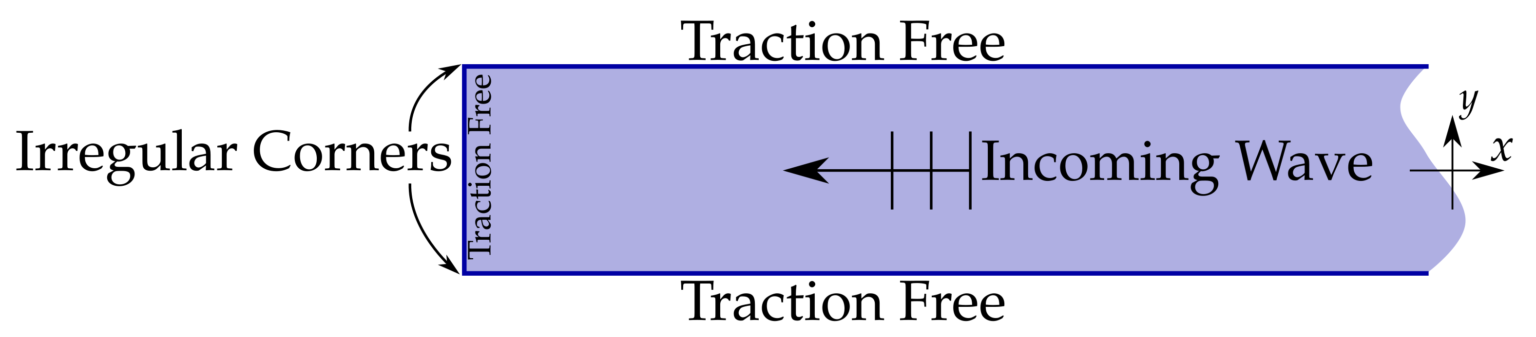
Figure 3.
The construction we use to implement corner modes. The shaded physical plate has traction free conditions on top and bottom, but the condition on the face will be applied later. The dashed lines denote an extended ‘virtual’ plate where we are imposing tractions on the surfaces which capture the correct local form of the stresses in the corners.
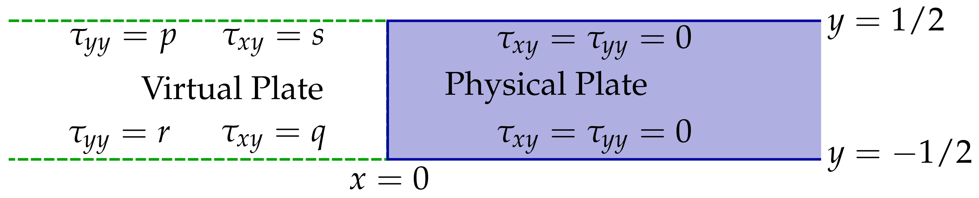
Figure 4.
A general traction-free elastic corner. The elastic body is the shaded area extending to infinity.
Figure 4.
A general traction-free elastic corner. The elastic body is the shaded area extending to infinity.
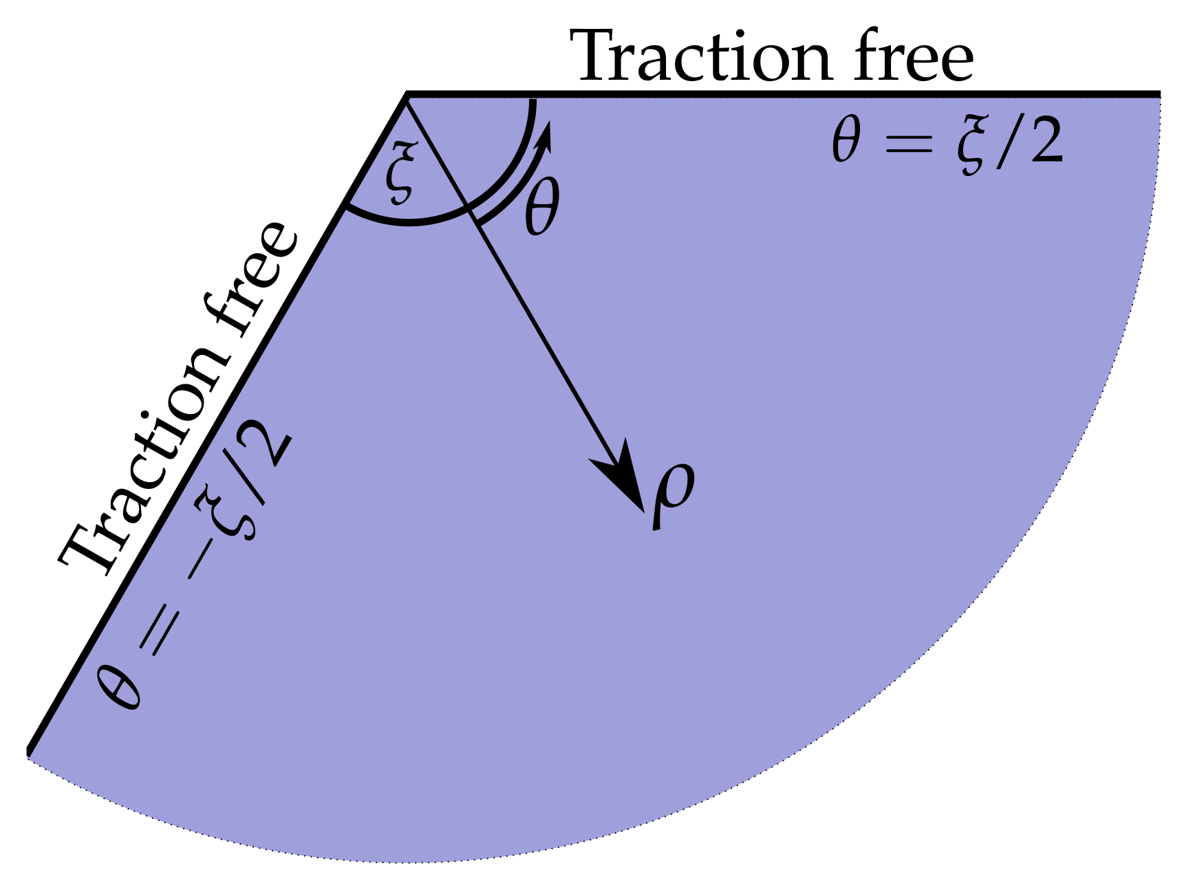
Figure 5.
Location of the virtual surfaces in terms of the local corner coordinate system for each corner.
Figure 5.
Location of the virtual surfaces in terms of the local corner coordinate system for each corner.
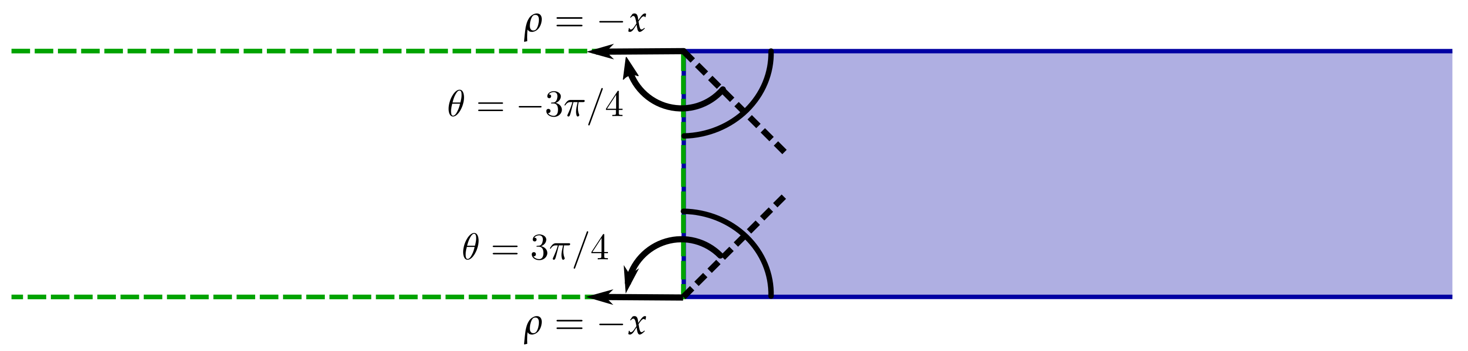
Figure 6.
Phase portrait of the function for , (left) and (right). It shows the location of the poles coinciding with the symmetric modes arising from the dispersion relation (21). The contours and extend horizontally to infinity. It can be shown that the functions decay for large and so the contribution of the contours connecting and at infinity can be neglected. The contours are chosen to take only the rightward propagating and/or decaying modes. The total number of poles between the two contours is what we call N. On the left plot, , and 1 of the 4 modes is propagating, while on the right plot , and 3 of the 12 modes are propagating.
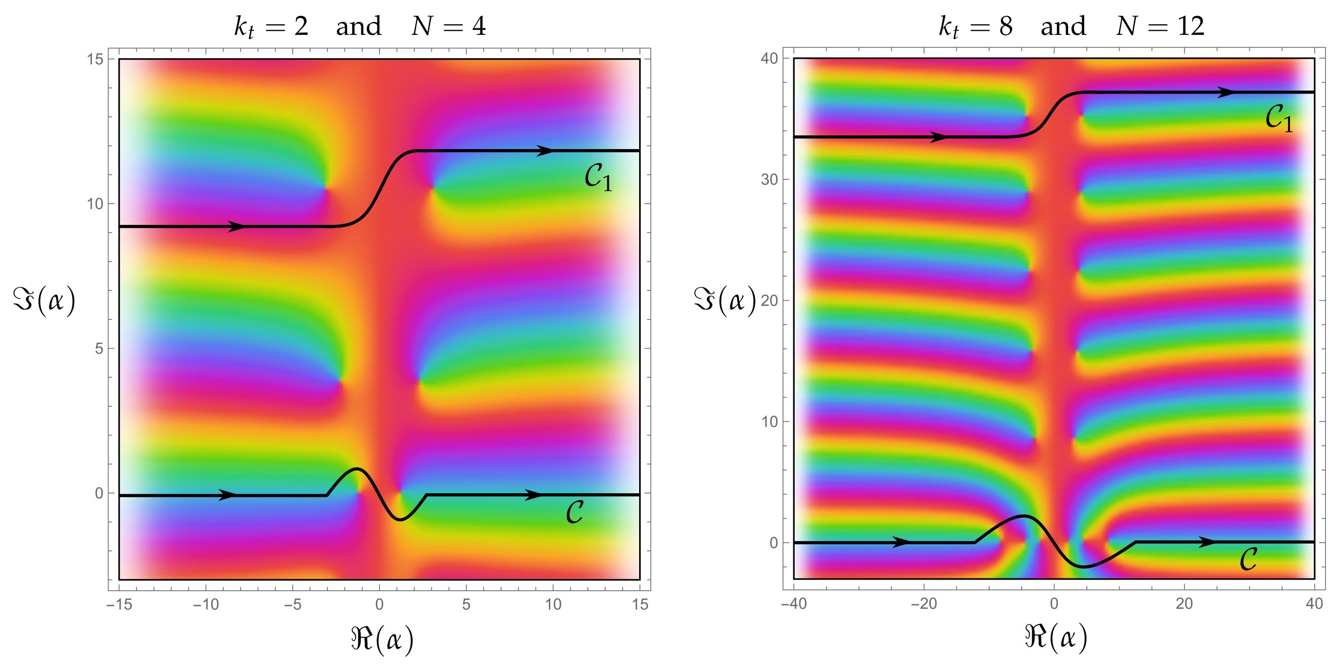
Figure 7.
The reconstructions of the stress fields using N symmetric Lamb modes and M corner modes. The curves correspond to: an expansion containing only Lamb waves, with ( ![Applsci 12 06468 i001]() ); a mixed expansion with and (
); a mixed expansion with and ( ![Applsci 12 06468 i002]() ); an expansion with and (
); an expansion with and ( ![Applsci 12 06468 i003]() ); and an expansion with and (
); and an expansion with and ( ![Applsci 12 06468 i004]() ). Subfigures (a,b) are the reconstructions of the scattered stress fields along the traction-free face. The negative of the incoming stress fields, which should lie on the same line, are plotted as (
). Subfigures (a,b) are the reconstructions of the scattered stress fields along the traction-free face. The negative of the incoming stress fields, which should lie on the same line, are plotted as ( ![Applsci 12 06468 i005]() ) for comparison. Subfigures (c,d) show the errors of the reconstructions of the total stress fields (sum of the incoming field and the outgoing field). In this example, and .
) for comparison. Subfigures (c,d) show the errors of the reconstructions of the total stress fields (sum of the incoming field and the outgoing field). In this example, and .
 ); a mixed expansion with and (
  ); an expansion with and (
  ); and an expansion with and (
  ). Subfigures (a,b) are the reconstructions of the scattered stress fields along the traction-free face. The negative of the incoming stress fields, which should lie on the same line, are plotted as (
  ) for comparison. Subfigures (c,d) show the errors of the reconstructions of the total stress fields (sum of the incoming field and the outgoing field). In this example, and .
Figure 7.
The reconstructions of the stress fields using N symmetric Lamb modes and M corner modes. The curves correspond to: an expansion containing only Lamb waves, with ( ![Applsci 12 06468 i001]() ); a mixed expansion with and (
); a mixed expansion with and ( ![Applsci 12 06468 i002]() ); an expansion with and (
); an expansion with and ( ![Applsci 12 06468 i003]() ); and an expansion with and (
); and an expansion with and ( ![Applsci 12 06468 i004]() ). Subfigures (a,b) are the reconstructions of the scattered stress fields along the traction-free face. The negative of the incoming stress fields, which should lie on the same line, are plotted as (
). Subfigures (a,b) are the reconstructions of the scattered stress fields along the traction-free face. The negative of the incoming stress fields, which should lie on the same line, are plotted as ( ![Applsci 12 06468 i005]() ) for comparison. Subfigures (c,d) show the errors of the reconstructions of the total stress fields (sum of the incoming field and the outgoing field). In this example, and .
) for comparison. Subfigures (c,d) show the errors of the reconstructions of the total stress fields (sum of the incoming field and the outgoing field). In this example, and .
); a mixed expansion with and ( ); an expansion with and ( ); and an expansion with and ( ). Subfigures (a,b) are the reconstructions of the scattered stress fields along the traction-free face. The negative of the incoming stress fields, which should lie on the same line, are plotted as ( ) for comparison. Subfigures (c,d) show the errors of the reconstructions of the total stress fields (sum of the incoming field and the outgoing field). In this example, and .
Figure 8.
A set of results showing the accuracy of the zero traction boundary condition for a variety of frequencies for fixed Poisson ratio . The maximum values of the incoming field for both tractions are order one. There is one propagating mode apiece for and 4, and three propagating modes when . The number of modes in each plot was chosen to maintain the same order of magnitude accuracy: for , and ; for , and ; and for , and .
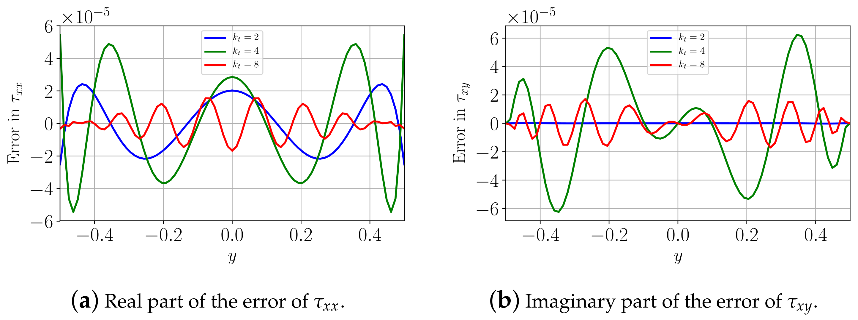
Figure 9.
For and (the most challenging case of Figure 8), we illustrate the convergence of the energy and of the reflection coefficients of the three propagating modes. We display the absolute error between the computed reflection coefficients and a reference value, i.e., that obtained for and , and the reference value for the energy is 1. The continuous lines correspond to the pure Lamb mode approach as the number N of Lamb modes increases. The dashed lines correspond to our new approach for a fixed number of Lamb modes as the number M of corner modes increases.
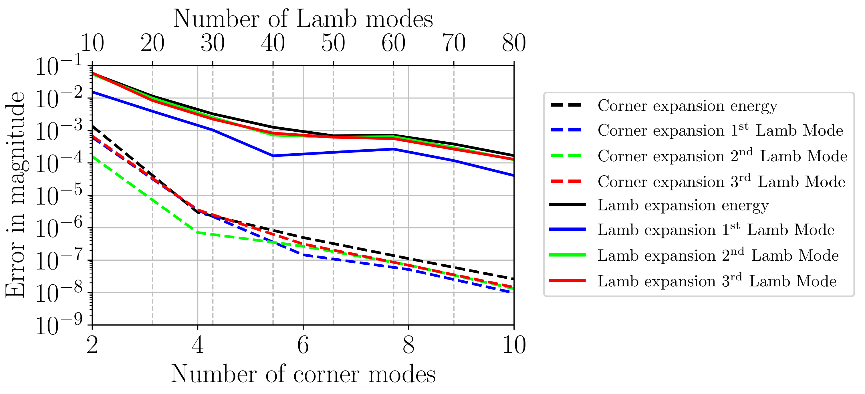
Figure 10.
The absolute value of the determinant of the collocation matrix, excluding the propagating mode, for different numbers of corner modes. The respective lines correspond to four Lamb modes and ( ![Applsci 12 06468 i001]() ), (
), ( ![Applsci 12 06468 i002]() ), (
), ( ![Applsci 12 06468 i003]() ), and (
), and ( ![Applsci 12 06468 i004]() ) corner modes. The dotted lines are the projected values of the determinant, found by extending the curves on either side of zero; this aids the determination of location of zero. The value of Poisson’s ratio at which the determinant vanishes can be seen to have converged, once or larger, to .
) corner modes. The dotted lines are the projected values of the determinant, found by extending the curves on either side of zero; this aids the determination of location of zero. The value of Poisson’s ratio at which the determinant vanishes can be seen to have converged, once or larger, to .
), ( ), ( ), and ( ) corner modes. The dotted lines are the projected values of the determinant, found by extending the curves on either side of zero; this aids the determination of location of zero. The value of Poisson’s ratio at which the determinant vanishes can be seen to have converged, once or larger, to .
Publisher’s Note: MDPI stays neutral with regard to jurisdictional claims in published maps and institutional affiliations. |
© Crown Owned Copyright AWE/MoD 2022. Licensee MDPI, Basel, Switzerland. This article is an open access article distributed under the terms and conditions of the Creative Commons Attribution (CC BY) license (https://creativecommons.org/licenses/by/4.0/).
Share and Cite
MDPI and ACS Style
Davey, R.C.; Assier, R.C.; Abrahams, I.D. An Efficient Semi-Analytical Scheme for Determining the Reflection of Lamb Waves in a Semi-Infinite Elastic Waveguide. Appl. Sci. 2022, 12, 6468. https://doi.org/10.3390/app12136468
AMA Style
Davey RC, Assier RC, Abrahams ID. An Efficient Semi-Analytical Scheme for Determining the Reflection of Lamb Waves in a Semi-Infinite Elastic Waveguide. Applied Sciences. 2022; 12(13):6468. https://doi.org/10.3390/app12136468
Chicago/Turabian StyleDavey, Robert C., Raphaël C. Assier, and I. David Abrahams. 2022. "An Efficient Semi-Analytical Scheme for Determining the Reflection of Lamb Waves in a Semi-Infinite Elastic Waveguide" Applied Sciences 12, no. 13: 6468. https://doi.org/10.3390/app12136468
Note that from the first issue of 2016, this journal uses article numbers instead of page numbers. See further details here.