Simultaneous DC Railway Power System Analysis Method Using Model-Based TPS

Abstract

This paper focuses on the development of a model-based train performance simulation with the practical train operation data using MATLAB Simulink. The developed program uses input operation data of a DC 1500 V metro line. And the simultaneous and multi-rate simulation for DC metro was performed to interface train schedule data with actual railway electrification system and vehicle. In the simulation, the voltage and power measured at each substation are provided during the traction, coasting and breaking mode. From this study, railroad vehicle load can be virtually modeled in the system internally and contribute to verifying new parts of the overall railway electrification systems.

1. Introduction

Recently, various next-generation electric vehicles and railroad systems are being introduced. Additionally, eco-friendly hydrogen railroad vehicles that cause low carbon, cause less fine dust pollution and energy cost reduction are being developed [1] in Korea. Meanwhile, in the traction power supply system (TPSS) sector, especially for DC metros, energy storage system (ESS) aided applications are one of notable research topics [2]. These topics require advanced understanding and representation of behavior of railroad vehicle loads.

Accurate modeling of railroad vehicle loads plays a very important role in analyzing the pre-verification of additional facilities, mainly vehicle electrical components, in the process. Among them, the train performance simulation (TPS) is an algorithm that obtains the train running time, traction and breaking power required for the input conditions of the electric power simulation by inputting vehicle data, track information, and other operating conditions [3]. Vehicle weight, train sets, acceleration, deceleration, auxiliary power, speed limit range, traction efficiency, braking efficiency, etc., are input as vehicle data, and curve and gradient, station location, and stop time are input as track data.

Conventional TPS was developer-friendly, script or code based design; the usage of the output are limited to component level. However, model-based design for TPS is user-friendly, and allows it to expand to a systematic level of design, which enables multi-environment simulation, test automation and easy to identify and correct errors. Above all, the main advantages of model-based design is that it can be a basis of prototyping technologies [4]. Prototyping technologies include HILS [5] and RCP, and those are required steps for system validation.

In these days, there are several state-of-art approach of railway vehicle speed profile calculation methods. References [6,7] gives an idea of using learning based methods. Furthermore, references [8,9] provides an on-line or real-time approach for train speed profile scheduling. Especially [9], which uses model predictive control, introduces a prediction and adjustment concepts. In this study, a model was developed based on the model-based TPS program, and its basic structures were well developed from previous studies [10,11,12,13]. Meanwhile, recently, as in reference [14], a TPS program has also been developed based on EMTDC for the TPSS protection field. Moreover, some previous studies in [15,16] provided basic concepts and structures using MATLAB Simulink for TPS. Especially, reference [15] is a well built TPS structure on MATLAB Simulink under the aforementioned TPS background computational technique. However, those earlier research works only covered a single itinerary between stations, or were limited to testing its performance, which does not cover it comprehensively.

The main contribution of this paper is as follows;

• This paper provides a complete form of model-based TPS, by solving practical computational issues.
• The model-based TPS results were verified with previous tools with C-scripts, and input data complies with universal requirements.
• Furthermore, simultaneous and multi-rates simulation of DC 1500 V metro with TPS is given at the end of this paper.

This paper consists of four parts; a background of train performance simulation is introduced in Section 2. Then, in Section 3, the structure of the mTPS is derived, and the mTPS simulation results are shown. The conclusion is followed in Section 5.

2. Background of the TPS Algorithm

Most of the railroad vehicles operate while maintaining a simple pattern of traction, coasting, braking and stopping modes. The train consumes traction power or generates regenerative power according to speed and position, and determines the next operating state and speed by obtaining acceleration and deceleration values. Accordingly, the vehicle has one driving state among each driving mode. That is, the next position is determined according to the speed of the train, and when the speed and position are determined, the operation curve and operation mode are determined as well. Additionally, this operation mode for moving vehicle load becomes an input data necessary for the circuit analysis of the TPSS.

2.1. Train Motion Equation

The acceleration that a train can produce is related to the traction force of the motor and the train resistance [17]. The acceleration of a train $a_i$, is the value obtained by dividing the effective traction force of $F_{eff}$ in kN by the dynamic mass of $m_{dyn}$ in tons, and it is expressed in Equation (1). The suffix i stands for calculation step for time, distance or velocity.

$$a_i=\frac{F_{eff,i}}{m_{dyn}}$$

(1)

Train set mass $m_{dyn}$ is a sum of the empty masses, inertial masses (for each type of the train) and passenger mass. Additionally, the inertial mass is an empty car mass times inertia coefficient. $F_{eff,i}$ can be expressed by subtracting the motor traction force $F_{mtf,i}$ from the train resistance $R_i$ in kN.

$$F_{eff,i}=F_{mtf,i}-R_i$$

(2)

and the $R_i$ consists of curve, running, and gradient resistance as Equation (3).

$$R_i=R_{Curve,i}+R_{Running,i}+R_{Gradient,i}$$

(3)

In the TPS algorithm, those train resistance values are calculated by referencing track information for specific train position. Additionally, the specific speed limits can be determined by the track information as well.

2.2. Calculation of TPS Dynamic

If the acceleration is given as Equation (1), then the time increment method can be expressed as

$$v_{i+1}=v_i+a\left(t_{i+1}-t_i\right)$$

(4)

$$s_{i+1}=s_i+v_i\left(t_{i+1}-t_i\right)$$

(5)

Next, the distance increment method can be expressed as below:

$$t_{i+1}=t_i+\frac{s_{i+1}-s_i}{v_i}$$

(6)

$$v_{i+1}=\sqrt{v_i^2+2a_i\left(s_{i+1}-s_i\right)}$$

(7)

Most of the previously developed program adopts the distance increment method. Note that, the time increment for distance increment method is not linear; it is a varying time step. Additionally, the velocity increment method can be expressed as

$$t_{i+1}=t_i+\frac{v_{i+1}-v_i}{a_i}$$

(8)

and $s_{i+1}$ is same as Equation (5).

Using Equation (5), the distance of the train moved is an integral of speed $v_i$ with respect to time. Which means that the turning point from coasting (or powering) to breaking mode must be given in time. So additional algorithm is needed to check if the train actually reached the destination as follows:

$$\left|D_k-\sum _{i=1}^N{d}_i^{\left(m\right)}\right|\le \sigma$$

(9)

where, $D_k$ is actual distance between two stations, $d_i^{\left(m\right)}$ is calculated distance between each adjacent modes i with regard to the selection of breaking points. This value can be acquired by taking the integral of a speed curve such as Figure 1.

Additionally, $\sigma$ is an arbitrary small number that guarantees the accuracy of the result.

However, additional iterative processes by adopting time increment method to satisfy Equation (9) can be an obstacle for simultaneous simulation. So, this paper uses a distance increment method. When using the distance increment method, time step changes by $\left(s_{i+1}-s_i\right)/v_i$. This is allowable from the point of view of the engineering because the time step for the railway power system, which is dominant, is much shorter than TPS time increment values. Additionally, as this paper focuses on varying resistance to represent moving train, evenly changing distance can be a reasonable choice and we will discuss this issue in the last section of the simulation part.

Forward and Backward Moving Calculation

There are two ways to acquire the turning point of breaking mode; manually or automatically. For designing purposes, manually putting on a notch signal, which controls the power of the train, can be used. However, this paper only focuses on the deriving automatic mode change of start, powering, coasting and braking status.

Simply, when the train moves forward by acceleration and backward by deceleration, that intersection point is a mode changing moment of coasting (or powering) to braking mode as shown in Figure 2. The forward calculation is literally that the train is moving from the previous station to the next target station. Meanwhile, the backward calculation is an assumption that the train is moving from the target station backwards to the previous station as Equations (10) and (11).

$$F_{eff,i}=F_{brk,i}+R_i$$

(10)

$$v_{b,i+1}=\sqrt{v_{b,i}^2-2a_{b,i}\left(s_{b,i+1}-s_{b,i}\right)}$$

(11)

For the distance integration of backward calculation, $s_{b,i+1}-s_{b,i}$ is negative value, so that the radicand of Equation (11) is positive. So the speed curve reversely increases as Figure 2a by the deceleration value of $a_{b,i}$. In short, the train virtually moves backwards to determine the exact breaking point of moving the train in forward direction.

The unique intersection point for breaking point calculation is shown in Figure 2b. Additionally, the Equation (12) represents the formula to calculate the unique intersection point of $\left(s_{c2b},v_{c2b}\right)$.

$$\left[\begin{array}{c}{s}_{c2b}\\ v_{c2b}\end{array}\right]={\left[\begin{array}{cc}{m}_f& -1\\ m_b& -1\end{array}\right]}^{-1}·\left[\begin{array}{c}{m}_f{s}_i-v_{f,i}\\ m_b{s}_i-v_{b,i}\end{array}\right]$$

(12)

The algorithm repeatedly finds the unique solution point using the forward slope $m_f$ and the backward slope $m_b$ acquired by adjacent points. For the example case of Figure 2, the intersection breaking point is 566.85 m, which is in between 566 and 567 m. Those floating point errors can be minimized by reducing distance increment value.

3. Development of Model-Based TPS Construction

3.1. Structure for Model-Based TPS

In this paper, a model based structure of TPS (mTPS) was built on the base framework developed in [15]. The computational requirements for mTPS includes:

• A scalable step size. (Scalability);
• Response capacity for abrupt advent of lower speed limit. (Adaptive);
• A compatibility between TPSS and train load. (Concurrency);
• Train stops and starts at the same position. (Continuity).

As shown in Figure 3, the entire program operates as a code that repeats operation according to the total location of the station information presented by the input data. Here, the input data includes station location, gradient, curve position, and traction or breaking force curves.

When the execution code is running, the braking point calculation model operates to receive TPS input data, and based on the information, the basic braking point is calculated and returned to the integrated model.

However, due to the operation structure of the TPS model that performs calculations per time sample, an unintended speed limit error may occur when the speed limit is changed as shown in Figure 4a. So an algorithm to correct the error has been added to correct those errors, and the result can be shown as Figure 4b.

3.2. DC Railway Power System Model

The voltage provided by KEPCO (Korea Electric Power Corporation) is set to 22.9 kV, 60 Hz. For three winding transformers, delta-delta-wye configuration selected to build DC 1500 V for rectifier output voltage. In this case, no load voltage is 1650 V, which is a practical value for the railway substation site. Figure 5 shows the schematic for the DC railway power system model under study. As the paper mainly focuses on the simultaneous mTPS and DC railway power system, circuit breaker (CB) models are not included. Figure 6 shows a circuit of moving train load using varying resistance.

Train movement by applying varying resistance is calculated as follows [18].

$$\left\{\begin{array}{c}\hfill R_{fwd,l}=R_{fwd}·\left(\left(d_{st}-d_A^{\ast }\right)+s_i\right)\hfill \\ \hfill R_{fwd,r}=R_{fwd}·\left(\left(d_B^{\ast }-d_{st}\right)-s_i\right).\hfill \end{array}\right.$$

(13)

$$\left\{\begin{array}{c}\hfill R_{ret,l}=R_{ret}·\left(\left(d_{st}-d_A^{\ast }\right)+s_i\right)\hfill \\ \hfill R_{ret,r}=R_{ret}·\left(\left(d_B^{\ast }-d_{st}\right)-s_i\right).\hfill \end{array}\right.$$

(14)

where, $R_{fwd}$ and $R_{ret}$ is forward rail resistance and return rail resistance in m$\Omega /$km, respectively. $d_{A,B}^{\ast }$ stands for the location of substation A and B. While $d_{st}$ is the previous station location. $s_i$ is the distance traveled by train. As the train moves towards the station, $R_{fwd,l}$ and $R_{ret,l}$ increases, and $R_{fwd,r}$ and $R_{ret,r}$ decreases by the rail resistance.

4. Train Performance Simulation Results

4.1. Model-Based TPS Description

Train specifications that used to express train motion using mTPS algorithm are provided in

Table 1. Input vehicle data for mTPS.

Quantity	Values	Quantity	Values
Weight	191 tons	Traction and breaking efficiency	0.91
$M_{dy}$	204 tons	Nominal voltage	1500 V
Set of train	4 trains (2M-2T 1-set)	Time step	0.5 s
Acceleration	3.0 km/h/s	Speed range	5 km/h
Deceleration	3.5 km/h/s	Dwell	30 s
Maximum speed	80 km/h	Scheduled speed	35 km/h

. The train set is 4 cars composed of two motor (M) cars and two train (T) cars each. The condition of track including curvature or gradient status are not provided, but included in the mTPS algorithm.

The traction motor

Table 2. Traction motor data for tractive effort curve.

Motor Data	Value	Quantity	Description
Total traction torque	18,105	kgf	-
Traction torque per motor	2263	kgf/motor	4 motors × 2 M-cars
Output power per motor	216	kW	Gear efficiency 0.975
Maximum output of traction motor	221	kW	at maximum acceleration
Input power of traction motor	283	kVA	at maximum acceleration

and traction effort curve in Figure 7 was designed to satisfy acceleration of 3.0 km/h/s at speed 35 km/h, with only $R_{Running}$ applied. That is, the condition validated for straight and flat (zero $R_{Curve,i}$ and $R_{Gradient,i}$) conditions for the rail section. For the traction effort curve (filled in blue area), there are three sections; constant torque, constant power and characteristic section, respectively.

In railway systems, voltage fluctuations are large due to moving train loads. So, when designing a traction substation, it is necessary to follow the voltage standards. IEC-60850 (Railway applications—Supply voltages of traction systems) proposes a range of voltage management standards specified in

Table 3. Supply voltages of DC 1500 V metro traction systems [19].

DC 1500 V Electrification System	Voltage (V)—DC (Mean Values)
Lowest non-permanent voltage	1000
Lowest permanent voltage	1000
Nominal voltage	1500
Highest permanent voltage	1800
Highest non-permanent voltage	1950

, which is specified in [19].

There are also standards for the duration of both ends of voltages. The duration of voltages between the lowest non-permanent and permanent voltages shall not exceed 2 min. Additionally, the duration of voltages between highest non-permanent and permanent voltages shall not exceed 5 min. The simulation condition complies with those requirements using DC breaking chopper; by setting activation voltage to 1800 V and shutdown voltage 1650 V. Additionally, the time duration for breaking mode doesn’t take up to 5 min in the simulation.

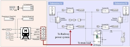
Using those specifications, the overall schematic structure for the model-based TPS is constructed as shown in Figure 8. The train moving model was partially used from previous research [20]. The program runs at multiple rates in time and distance. First, the mTPS model is represented in the top; the red box has $\Delta$s = 0.5 s and varying $T_s$. Where the $\Delta$s stands for increment of distance. The cause of varying time step $T_s$ has been described at Section 2.2.

The rail, contact line and train schematic shown on the bottom; in blue box, $T_{s2}=0.001$ s. Each of them represents a series of connected DC substations, with varying resistance to show mTPS applied train load moving along the entire DC metro line for 11-station, simultaneously.

4.2. Model-Based TPS Results

4.2.1. mTPS Result and Dynamic Behavior of Train

Figure 9 shows the results of the mTPS introduced earlier. By adopting the distance integration method of Reference [10], it is first output as a curve for distance, so that time has the same concept as distance in simulation. Additionally, as shown in Figure 9a, it can be seen that the case where the speed exceeds the speed limit does not occur by performing the error correction mentioned in the previous section. This was corrected by repeatedly adjusting the coasting point. In addition, it can be observed that the departure time and point and arrival time and point are accurately reflected because all the braking point calculation models are considered. Figure 9b shows the power consumption and production at the train. In powering mode, the train approximately consumes 2 MW and in breaking mode the train produces less than 3 MW.

Before observing voltages and power for substation A and B, Figure 10 shows corresponding region of speed and acceleration values. Note that the x-axis is marked in time quantity, not distance.

In the speed-time curve, there is a dwelling time for 30 s, so the train stops at the station. It is clear that the acceleration is around 3.0 km/h/s at a speed of 35 km/h, which is defined in Figure 7. Those changing points are formed due to the vehicle driving mode changing from constant torque to constant power mode. Meanwhile, some differences were made due to train curve or gradient resistance.

4.2.2. Simultaneous DC Railway Power System Simulation

In this section, an effect of traction and breaking motion on DC railway power system especially voltage aspect are introduced. The location for substations are marked in Figure 9a, and the study region of this paper is between substation A and B.

Figure 11a shows the result of the power aspect of the 1500 V dc metro system with mTPS. Most of the train has an auxiliary power so the power-time curve is biased for 130 kW. Figure 11b represents the voltage at the substation A (red line) and B (blue line). Obviously, the rise of voltage is observed during breaking mode, but as the braking chopper operates it is limited to 1800 V. And for the powering section, the voltage drops due to approximately 2 MW train load. Specifically, when the train is in powering mode, the voltage is higher near substation A and vice versa. Its obvious because the train load current travels a shorter distance than the opposite side substation.

Figure 12 shows a comparison between sum of power of substation A, B and train load power in time. Sum of power produced by substation A, B in traction mode is the same as the train power load. However, as the breaking chopper operates at breaking mode, substations do not supply any power to the train. In short, comparing the second figure of Figure 11 and Figure 12, observing at the substation aspect, at breaking mode and coasting mode, substation has no load condition, therefore the voltage rises up to DC 1800 V. So, the voltage might drop when using breaking power as a regenerative power.

5. Discussion

Speed result of legacy codes (code A and B) of KRRI (Korea Railroad Research Institute) in C script have been compared in Figure 13. Figure 13a shows a partial result for speed profile. Comparing legacy codes, the mTPS have a more uniform speed range of 5 km/h.

As shown in Figure 13b, mTPS has 11,066 points of speed data, code A and B only has 902 and 897 points of speed data when time step was set to 1 s for same vehicle and track conditions. This result is obvious because mTPS samples all 11 km length of journey in meters. If the constant time increment is required, mTPS can allow down sampling function or block to acquire time increment method based results. Furthermore, using distance increment based mTPS, the linear change in distance takes advantage of applying train moving models or varying resistance. Additionally, for validation, when comparing cite information using the DAQ system, mTPS results can be adjusted by applying down-sampling in time. Meanwhile, there can be some validation considerations or limitations—provisional errors of mTPS in the future. First, as the operator’s driving pattern is not standardized, there can be expected errors during validation. Next, the mixture of air breaking system and electrical (regenerative) breaking system is not included in this paper. Finally, some minor portion of losses or efficiencies are ignored.

6. Conclusions

In this study, a mTPS program was constructed based on the MATLAB Simulink program. Additionally, the speed and traction and breaking power profiles as well as voltage profiles were obtained for the entire route (one-way) for DC 1500 V metro line. The main contribution of this paper is summarized as follows:

• The mTPS provides fully integrated performance with input vehicle and track data.
• The mTPS results complies with reasonable requirements.
• The mTPS can provide detailed dynamics of the train comparing previous TPS works.
• Simultaneous multi-rates simulation of DC metro with mTPS were shown in the previous section.

Further work includes an improvement of the accuracy and temporal resolution of the model produced from this study. So, our final target for train load modeling is to use the mTPS as a single, universal model in OPAL-RT framework for virtual commissioning such as propulsion inverters such as VVVF inverters or DC/DC converters for on-board railway vehicles. At the same time, we plan to integrate it into the hydrogen-supplied train and locomotive model and develop it into a hybrid computation model so that it can be directly used in real-time simulation.

References

- Lee, J.; Ryu, J. Hydrogen Fuel-Cell/Battery Hybrid Train. J. Korean Soc. Railw. 2019, 22, 19–26. [Google Scholar] [CrossRef]
- Yang, Z.; Yang, Z.; Xia, H.; Lin, F. Brake Voltage Following Control of Supercapacitor-Based Energy Storage Systems in Metro Considering Train Operation State. IEEE Trans. Ind. Electron. 2018, 65, 6751–6761. [Google Scholar] [CrossRef]
- Goodman, C.; Siu, L.; Ho, T. A review of simulation models for railway systems. In Proceedings of the 1998 International Conference on Developments in Mass Transit Systems, London, UK, 20–23 April 1998; Volume 543, pp. 80–85. [Google Scholar]
- Oh, H. Model Based Design application for Power electronics development. Korean Inst. Electr. Eng. 2021, 70, 15–22. [Google Scholar]
- Liu, C.; Guo, X.; Ma, R.; Li, Z.; Gechter, F.; Gao, F. A System-Level FPGA-Based Hardware-in-the-Loop Test of High-Speed Train. IEEE Trans. Transp. Electrif. 2018, 4, 912–921. [Google Scholar] [CrossRef]
- Ning, L.; Zhou, M.; Hou, Z.; Goverde, R.M.; Wang, F.Y.; Dong, H. Deep Deterministic Policy Gradient for High-Speed Train Trajectory Optimization. IEEE Trans. Intell. Transp. Syst. 2021, 1–13. [Google Scholar] [CrossRef]
- Zhou, K.; Song, S.; Xue, A.; You, K.; Wu, H. Smart Train Operation Algorithms Based on Expert Knowledge and Reinforcement Learning. IEEE Trans. Syst. Man, Cybern. Syst. 2022, 52, 716–727. [Google Scholar] [CrossRef]
- Xiao, Z.; Wang, Q.; Sun, P.; Zhao, Z.; Rao, Y.; Feng, X. Real-Time Energy-Efficient Driver Advisory System for High-Speed Trains. IEEE Trans. Transp. Electrif. 2021, 7, 3163–3172. [Google Scholar] [CrossRef]
- Zhong, W.; Li, S.; Xu, H.; Zhang, W. On-Line Train Speed Profile Generation of High-Speed Railway With Energy-Saving: A Model Predictive Control Method. IEEE Trans. Intell. Transp. Syst. 2022, 23, 4063–4074. [Google Scholar] [CrossRef]
- Jong, J.C.; Chang, S. Algorithms for generating train speed profiles. J. East. Asia Soc. Transp. Stud. 2005, 6, 356–371. [Google Scholar]
- Hwang, H.S. Control strategy for optimal compromise between trip time and energy consumption in a high-speed railway. IEEE Trans. Syst. Man Cybern. Part A Syst. Hum. 1998, 28, 791–802. [Google Scholar] [CrossRef]
- Wong, K.K.; Ho, T.K. Dynamic coast control of train movement with genetic algorithm. Int. J. Syst. Sci. 2004, 35, 835–846. [Google Scholar] [CrossRef] [Green Version]
- Zhao, N.; Roberts, C.; Hillmansen, S.; Western, P.; Chen, L.; Tian, Z.; Xin, T.; Su, S. Train trajectory optimisation of ATO systems for metro lines. In Proceedings of the 17th International IEEE Conference on Intelligent Transportation Systems (ITSC), Qingdao, China, 8–11 October 2014; pp. 1796–1801. [Google Scholar]
- Lee, H.; Kim, J.; Lee, C.; Kim, J.R.; Jang, G. Numerical Analysis Model on PSCAD/EMTDC for Train Performance Simulation. In Proceedings of the The 51st Summer Conference of the Korean Electrical Society in 2020, Busan, Korea, 15–17 July 2020; pp. 2012–2013. [Google Scholar]
- Kang, M.; Han, M. A Train Performance Simulation using Simulink for Generating Energy-efficient Speed Profiles. Trans. Korean Inst. Electr. Eng. 2010, 59, 1816–1822. [Google Scholar]
- Nitsch, A.; Beichler, B.; Golatowski, F.; Haubelt, C. Model-based Systems Engineering with Matlab/Simulink in the Railway Sector. In Proceedings of the MBMV 2015, Chemnitz, Germany, 3–4 March 2015. [Google Scholar]
- Brenna, M.; Foiadelli, F.; Zaninelli, D. Electrical Railway Transportation Systems; IEEE Press Series on Power and Energy Systems; Wiley: Hoboken, NJ, USA, 2018. [Google Scholar]
- Alnuman, H.; Gladwin, D.; Foster, M. Electrical Modelling of a DC Railway System with Multiple Trains. Energies 2018, 11, 3211. [Google Scholar] [CrossRef] [Green Version]
- Railway Applications—Supply Voltages of Traction Systems; International Standard, International Electrotechnical Commission: Geneva, Switzerland, 2014.
- Saleh, M.; Dutta, O.; Esa, Y.; Mohamed, A. Quantitative analysis of regenerative energy in electric rail traction systems. In Proceedings of the 2017 IEEE Industry Applications Society Annual Meeting, Cincinnati, OH, USA, 1–5 October 2017; pp. 1–7. [Google Scholar]
Figure 1.
Determination of train arrival by Equation (5).
Figure 2.
Breaking point decision by forward and backward moving calculation. (a) Breaking point decision—Forward and backward calculation yield intersection point. (b) Intersection calculation for breaking point determination—magnified figure for Figure 2a.
Figure 3.
Computational procedure of mTPS.
Figure 4.
Speed error correction method for mTPS. (a) Speed error correction method. (b) An example of speed error correction.
Figure 5.
Schematics of moving train load using varying resistance.
Figure 6.
Circuit of moving train load using varying resistance.
Figure 7.
Traction and breaking effort curve under study.
Figure 8.
Developed mTPS and TPSS model.
Figure 9.
mTPS result for train dynamic representation. (a) Distance versus speed curve for DC metro line and substation location. (b) Distance versus traction and breaking power curve.
Figure 10.
Train speed and acceleration result in time;section between substation A and B.
Figure 11.
Train power load and voltages of substation A, B in time. (a) Train power load traveling between substation A, B. (b) Voltage measured at substation A, B while the train moves.
Figure 12.
Comparison between sum of power of substation A, B and train load power in time.
Figure 13.
Verification of mTPS with legacy codes. (a) Comparative study for mTPS result and code A, B. (b) Magnified figure for Figure 13a.