Abstract
Currently, the field of transparent image analysis has gradually become a hot topic. However, traditional analysis methods are accompanied by large amounts of carbon emissions, and consumes significant manpower and material resources. The continuous development of computer vision enables the use of computers to analyze images. However, the low contrast between the foreground and background of transparent images makes their segmentation difficult for computers. To address this problem, we first analyzed them with pixel patches, and then classified the patches as foreground and background. Finally, the segmentation of the transparent images was completed through the reconstruction of pixel patches. To understand the performance of different deep learning networks in transparent image segmentation, we conducted a series of comparative experiments using patch-level and pixel-level methods. In two sets of experiments, we compared the segmentation performance of four convolutional neural network (CNN) models and a visual transformer (ViT) model on the transparent environmental microorganism dataset fifth version. The results demonstrated that U-Net++ had the highest accuracy rate of 95.32% in the pixel-level segmentation experiment followed by ViT with an accuracy rate of 95.31%. However, ResNet50 had the highest accuracy rate of 90.00% and ViT had the lowest accuracy of 89.25% in the patch-level segmentation experiments. Hence, we concluded that ViT performed the lowest in patch-level segmentation experiments, but outperformed most CNNs in pixel-level segmentation. Further, we combined patch-level and pixel-level segmentation results to reduce the loss of segmentation details in the EM images. This conclusion was also verified by the environmental microorganism dataset sixth version dataset (EMDS-6).
1. Introduction
With the advent of science and technology, the application of transparent images has increasingly been used in various fields around humans, such as the segmentation of renal transparent cancer cell nuclei in medicine [1]. The shape and location information of the cell nucleus are of great significance in the segmentation and diagnosis of benign and malignant tumors [2,3]. Another example is the identification of the number of transparent microorganisms in an environment to determine the degree of environmental pollution [4]. In recent years, the segmentation of transparent objects in images has become a hot topic in vision research [5,6]. It is not easy to detect whether there are transparent or translucent objects in the images because the transparent object area to be observed is generally small or thin, and the colors and contrasts of the foreground and background are similar [7]. Only the residual edge can lead to a low resolution of the foreground or background, which largely depends on the background and lighting conditions. Therefore, there is an urgent need for effective methods for identifying transparent or translucent images.
In recent years, deep learning has achieved a good performance in the field of computer vision. We consider the excellent performance of computer vision in image analysis [8], such as its high speed, high accuracy, low consumption, high degree of quantification, and strong objectivity [9]. Additionally, compared with traditional manual methods, computer image analysis can reduce manual effort from time-consuming tasks. Consequently, computer vision-based approaches can overcome the limitations of traditional methods and demonstrate great potential for transparent image analyses [10]. Particularly, when the object is transparent or has low contrast in the image, more foreground information is required; therefore, more visual details are found to recover the lost information from patches or pixels. As shown in Figure 1, the foreground and background of microorganisms are similar. There is only a small amount of information on the edges; which makes it difficult for traditional convolutional neural network (CNN) algorithms to distinguish transparent objects in images globally [11]. To address this problem, it is necessary to analyze transparent images from patches. We cropped the image into fixed-size patches and created a deep learning network to learn the features of the visual information of foreground and background patches. The network trained in this manner is sensitive to the foreground and background, which helps to distinguish transparent objects and achieve segmentation.
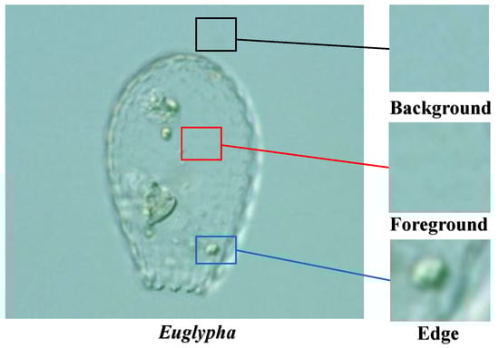
Figure 1.
An example of transparent images (a low contrast environmental microorganism image).
In recent years, machine vision has been widely used for image processing [12,13]. Deep learning is a more effective method in the field of machine vision, such as the popular Convolutional Neural Network (CNN) Xception, VGG-16, Resnet50, Inception-V3, U-Net, and novel Visual Transformers (ViT) [14]. CNNs gradually expand the receptive field by increasing the size of the convolution kernel until it covers the entire image; thus, CNNs complete the image extraction from local to global information. Contrarily, transformers can obtain global information from the beginning, making learning more challenging, but their ability to retain long-term dependence is more potent than that of CNN [15]. Therefore, CNNs and transformers have both advantages and disadvantages when handling visual information. Therefore, this study compares the patch-level and pixel-level segmentation performance of transparent images with different CNN and visual transformer methods. This study aims to determine the adaptability of various deep learning models in this research domain.
The main contributions of this paper are as follows:
(1) A comparative study on patch-level transparent image segmentation was conducted to help analyze transparent images.
(2) The segmentation performances of multiple CNN and ViT deep learning networks under patch-level and pixel-level images were compared, which is convenient in performing further ensemble learning.
2. Related Work
This section briefly introduces related research on transparent images in practical analysis tasks and classical deep learning models.
2.1. Introduction to Transparent Image Analysis
Object analysis is one of the essential branches in robot vision; particularly, the analysis of transparent images of objects (transparent images) is challenging [16]. In the traditional machine learning method, the multiclass fusion algorithm can only extract the shallow features of a transparent image, and the obtained feature layer is incomplete. Practically, it is difficult for multiclass fusion algorithms to detect transparent objects. For example, home robots cannot see objects at all when they detect transparent glassware. The ClearGrasp machine learning algorithm performs well in analyzing transparent objects [17]. It can estimate the high-precision data of transparent objects from RGB-D transparent images, thereby improving the accuracy of transparent object detection.
Photoelectric sensors are widely used in industrial automation, mechanization, and intelligence as a necessary technical means for analyzing objects. In [18], it uses the properties of light to detect the position and changes of an object. Sensors and smart systems are used to separate recyclable materials (transparent materials and metals) into different bins, without using manpower.
There are many transparent objects in the industrial field, such as transparent plastics, colloids, and liquid drops. These transparent objects bring considerable uncertainty to products. For factories to have high-quality products, it is sometimes essential to analyze these transparent objects and control their shapes. However, it is difficult to segment the shapes of transparent objects using morphological methods. For instance, Hata et al. used a genetic algorithm to segment a transparent paste-drop-shape in the industry and obtained good performance [19].
Segmentation of transparent objects is significantly useful for computer vision applications. However, the foreground of a transparent image is usually similar to its background environment, which leads to commonly used image segmentation methods handling transparent images generally. The light-field image segmentation method can accurately and automatically segment transparent images with a small depth-of-field difference and improve the accuracy of the segmentation with less calculations [20]. Hence, they are widely used for the segmentation of transparent images.
The correct segmentation of zebrafish in biology has extensively promoted the development of the life sciences. However, zebrafish transparency makes the edges blurred during segmentation. The mean-shift algorithm can enhance the color representation in the image and improve the discrimination of the specimen against the background [21]. This method improves the efficiency and accuracy of zebrafish specimen segmentation.
Visual object analysis is vital for robotics and computer vision applications. Commonly used statistical analysis methods, such as the bag-of-features, are often applied to image segmentation [22]. The principle is to extract local features of the image for segmentation. However, the foreground transparent objects in transparent images do not have complete features; therefore, it is difficult to accurately segment transparent images. The more popular method is the light field distortion feature [23], which can describe transparent objects without knowing the texture of the scene, thus improving the segmentation accuracy of transparent images.
2.2. Introduction Classic of Deep Learning Network Models
Simonyan et al. proposed a VGG series of deep learning network models (VGG-Net), of which VGG-16 is the most representative [24]. VGG-Net can imitate a larger receptive field by using multiple filters, enhancing nonlinear mapping, reducing parameters, and improving the network to better its analytics. Meanwhile, VGG-16 continues to deepen the previous VGG-Net with 13 convolutional layers and three fully connected layers. With a continuous increase in the convolution kernel and convolution layer, the nonlinear ability of the model becomes stronger. VGG-16 can better learn the features in images and achieve good performance in image classification, segmentation, and detection. Simonyan proved that as the depth of the network increases, the accuracy of the image analysis increases [24]. Nevertheless, this increase in depth is limited. An excessively increase in the depth of the network may lead to network degradation problems. Therefore, the optimal network depth of the VGG-Net is set to 16–19 layers. Moreover, VGG-16 has three fully connected layers, which causes more memory to be occupied, a long training time, and difficulty in tuning the parameters.
He et al. proposed a ResNet series of networks and added a residual structure in the networks to solve the problem of network degradation [25]. The ResNet model introduces the jumpy connection method (shortcut connection). This connection method allows the residual structure to skip levels that are not fully trained in the feature extraction process and increases the model’s utilization of feature information during the training process. As the most classical model in the ResNet series, ResNet50 has a 50-layer network structure. This model adopts a highway network structure, which allows the network to have strong expression capabilities and acquire more advanced features. Therefore, it is widely used in image analysis. However, the network model is significantly deep and complicated; therefore, determining the layers in the deep network that are not thoroughly trained and then optimizing the network is a complex problem.
Szegedy et al. proposed a GoogLeNet network model, which has the advantage of reducing the complexity of networks based on ResNet. They first proposed Inception-V1, whose network is 22 layers deep and comprises multiple inception structure cascades as basic modules; each inception module consists of a , , convolution kernel and a maximum pooling, which is similar to the idea of multiscale, and increases the adaptability of the network to different scales [26]. With the continuous improvement of the inception module, the Inception-V2 network uses two convolutions instead of convolutions. This improves the Batch Normalization (BN) method, which rescales the data distribution to accelerate the model convergence [27]. Inception-V3 network introduces the idea of decomposing convolution, splitting a larger two-dimensional convolution into two smaller one-dimensional convolutions, further reducing the number of calculations [28]. Concurrently, Inception-V3 optimizes the inception module, embeds the branch in the branch, and improves the model’s accuracy.
Xception is another improvement after Inception-V3 [29]. It mainly uses depthwise separable convolution to replace the convolution operation in Inception-V3. The Xception model uses deep separable convolution to increase the width of the network, which improves the accuracy of the classification and ability to learn subtle features. Xception adds a residual mechanism similar to ResNet to significantly improve the speed of convergence during training and accuracy of the model. However, Xception is relatively fragmented during the calculation process and results in a slower iteration speed during training.
U-Net is a CNN that was initially used to perform medical image segmentation. The U-Net architecture is symmetrical. It comprises a contracting and an expansive paths [30]. U-Net makes two significant contributions. The first is the extensive use of data augmentation to solve the problem of insufficient training data. The second is its end-to-end structure, which can help the network retrieve information from the shallow layers. Owing to its outstanding performance, U-Net has been widely used in semantic segmentation.
The transformer is a deep neural network based on the self-attention mechanism, enabling the model to be trained in parallel and obtain global information from the training data. Owing to its computational efficiency and scalability, it is widely used in natural language processing (NLP). Recently, Dosovitskiy et al. proposed a vision transformer (ViT) model that performs significantly well in image classification tasks [31]. In the first training step, the ViT model divides pictures into fixed-size image patches and uses their linear sequence as the input of the transformer model. In the second step, position embeddings are added to the embedding patches to retain the position information, and the image features are extracted through the multihead attention mechanism. Finally, the classification model is trained. ViT overcomes the limitation that the CNN model cannot be calculated in parallel, and self-attention can produce a more interpretable model. ViT is suitable for solving image-processing tasks, but experiments have proven that large data samples are required to improve the training effect.
Currently, deep learning methods are used to solve practical application problems in various fields. For example, in [32], a deep learning model was developed to detect and track sperm, which can effectively assist doctors in determining male reproductive health. In [33,34,35,36], a deep learning network is used to identify areas of cervical cancer that helps doctors to analyze cervical histopathological images. Owing to the spread of coronavirus disease 2019 (COVID-19), medical resources have continuously been depleted. In [37], the detection performance of 15 different deep learning models for COVID-19 X-ray image identification are compared, which can help reduce the workload of doctors. In [38], a multiple network model was proposed for the analysis of intracranial pressure (ICP) and heart rate (HR) after severe traumatic brain injury in pediatric patients. In [39], to help pathologists detect cancer subtypes and genetic mutations, a deep learning model was developed. In [40], to predict the response to immune checkpoint inhibitors in advanced melanoma and effectively assist doctors in diagnosis, a deep learning model was trained on clinical data. In [41], machine-learning methods are used to investigate, predict, and discriminate COVID-19.
3. Comparative Experiment
This section introduces patch-level and pixel-level segmentation experiments and the segmentation results of transparent images under several deep learning networks. The patch-level and pixel-level image segmentation workflows are shown in Figure 2.
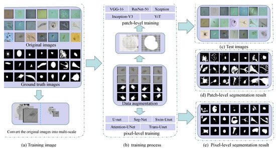
Figure 2.
Workflow of patch-level and pixel-level segmentation in transparent images (using environmental microorganism EMDS-5 images as examples) ((a) is the image of the training set and the grayscale of the original image. (b) is the patch-level and pixel-level training process. In (c) is the test set image. (d,e) are patch-level and pixel-level segmentation results, respectively).
3.1. Experiment Setting
3.1.1. Data Settings
In this study, we used the environmental microorganism dataset fifth version (EMDS-5) as transparent images for the analysis [4]. The effectiveness and robustness of deep learning methods based on the small dataset, EMDS-5, are provided in detail in [42]. Table 1 shows the data distribution of EMDS-5 in the experiment. It is a newly released version of the EMDS series, which includes 21 types of EMs, each of which contains 20 original microscopic images and their corresponding ground-truth (GT) images (examples are shown in Figure 3). We randomly divided each category of the EMDS-5 into training, validation, and test datasets in a ratio of 1:1:2. Thus, we obtained 105 original images and their corresponding GT images for training and validation, respectively, and 210 original images for testing.

Table 1.
EMDS-5 experimental data setting.
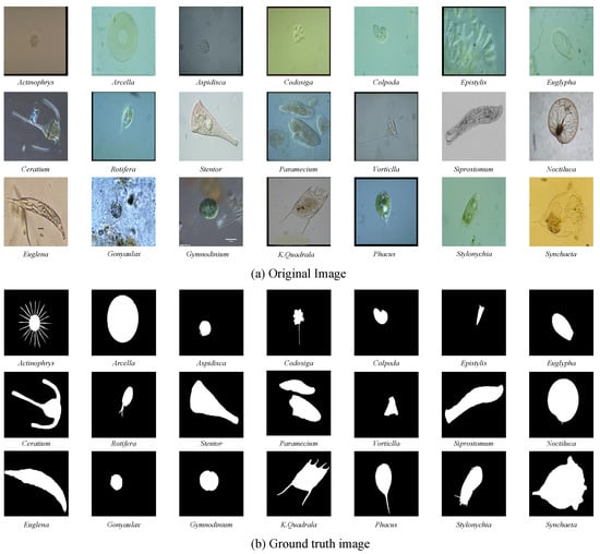
Figure 3.
Examples of the environmental microorganism image in EMDS-5. (a) is the original images of EMDS-5, each image contains one or more EM objects of the same species, and one image is selected for each species as a representative. (b) correspond to the real segmentation images of microorganisms in each image in the (a). The pixel value of the background part in the microorganism image is set to 0, and the foreground part is set to 1.
3.1.2. Data Preprocessing
Patch-Level Data Preprocessing
In the first step, considering that the light source had a significantly large effect on the color of the microscope image and that the same sample show different colors under different light sources, the color information was less important for the sign extraction of the microscopic image [43]. Therefore, we converted the EM microscopic images into grayscale to reduce the computational workload of the network model. In the second step, we converted all image sizes into pixels because the microscopic images were of various sizes. In the third step, the training and validation images, and their corresponding GT images were cropped into patches ( pixels), and = 107,520 patches were obtained. Based on the corresponding GT image small patches, we divided these small patches into two categories: foreground and background. The partition criterion was based on whether the area of interest in the patch comprises half of the entire patch. If so, we assigned the foreground as the label of this patch; otherwise, it was annotated as the background. Finally, we found that the pixel patches with foreground and background were 16,554 and 90,966, respectively. During the training process, we found that the model weights were heavily biased towards negative samples owing to the imbalance between positive and negative samples. To avoid data imbalance during training, we rotated the training set image small patches by 0°, 90°, 180°, and 270°, and mirrored them for data augmentation. We then further obtained 16,544 = 132,432 patches, from which 90,966 patches were randomly selected as the patches that were finally used in the training set. Details of the image patches are listed in Table 2.
Table 2.
Patch-Level data preprocessing. FG (foreground) and BG (background).
Pixel-Level Data Preprocessing
The image was converted to grayscale and resized to pixels for the pixel-level segmentation experiments.
3.1.3. Hyper Parameters
The patch-level experiment used the Adam optimizer with a learning rate of 0.0002, and the batch size was set to 32. During the training, we used the cross-entropy loss function to optimize the deep learning model [44]. Figure 4 shows the accuracy and loss curves of the different deep learning models used in this experiment. The epoch was determined based on the convergence of the loss curve. In our pretest, we tried to train 100 epochs and maintained the best training model weights, and found that the best model appeared between 40 and 50, where too much training caused overfitting and too little training was not able to train the optimal model. Therefore, considering the computational performance of the workstation, we finally set 50 epochs for training. Deep neural networks have a strong expressive ability compared to traditional models that require more data to avoid overfitting. Because our experiment was conducted on a small dataset, we employed a transfer learning approach to avoid the overfitting problem [45]. Meanwhile, because of the outstanding classification ability of CNN in ImageNet and the significant performance of transfer learning with a limited training data set [24], we used the limited EM training data to fine-tune the CNN model pretrained by ImageNet [46,47]. It has been proven that using CNN pretrained on ImageNet is useful for classification tasks through the concept of transfer learning and fine-tuning [48]. Before fine-tuning the pretrained CNN, we froze the parameters of the pretrained model. Subsequently, we used patch-level data to fine-tune the dense layers of the CNN. We retained the backbone network of the CNN classification network to extract image features and replace the last fully connected layer of the CNN model with Global Average Pooling2D + dense + dense + SoftMax. Global average Pooling2D simplifies many parameter operations. The purpose of the dense layer is to extract the correlation between these features through nonlinear changes in the dense layer and map them to the output space. Finally, the class probability result was outputted using SoftMax. We also compared the validation set accuracy of the ViT model with and without pre-trained weights. In both sets of experiments, we trained three times and then averaged the results. We found that ViT without pretrained weights and ViT with ImageNet pretrained weights had accuracies of 0.8923 and 0.8926 on the validation set, respectively. During training, ViT takes approximately 2G less memory for loading than the ImageNet pretrained weight model. To compare the performance of the two methods, we used ViT without pretraining as the optimization option. We set the network depth to six, heads to 16, mlp_dim to 3000, and dropout and emb_dropout to 0.1. The pixel-level experiment used the Adam optimizer with a learning rate of 0.001, and the batch size was set to 4. Figure 5 shows the loss curves of the different deep learning models in this experiment. The training curves began to converge after 90 epochs of iterations for the five models. To prevent overfitting, we set 100 epochs for training.
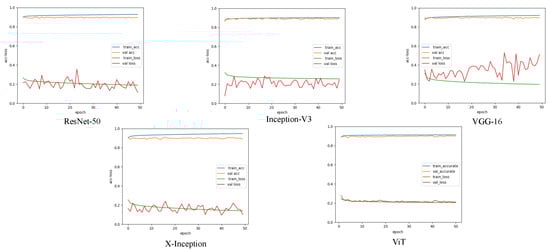
Figure 4.
A comparison of the image segmentation results of the loss and accuracy curves of deep learning on pixels training and validation sets. (Each legend has four curves, respectively, the accuracy and loss values of the training set, and the accuracy and loss values of the validation set).
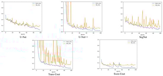
Figure 5.
A comparison of the image segmentation results of the loss curves of deep learning on pixel-level training and validation sets.
3.2. Evaluation Metrics
To compare the classification foreground and background performances of different methods, we used the commonly used deep learning classification indexes—accuracy (Acc), precision (Pre), recall (Rec), specificity (Spe), and F1-Score (F1)—to evaluate the patch-level results [49]. Acc reflects the ratio of correct classification samples to total samples. Pre reflects the proportion of correctly predicted positive samples in the model classification of positive samples. Rec reflects the correct proportion of model classification for all positive samples. Spe reflects the proportion of the model that correctly classifies negative samples among the total negative samples. F1 is a calculation result that comprehensively considers the Pre and Rec of the model. In addition, we employed Dice, Jaccard, Pre, Acc, and Rec to evaluate the results of pixel-level segmentation [38]. V represents the foreground predicted by the model. V represents the foreground in the ground-truth image. From Table 3, we can determine that the higher the values of the first four metrics (Dice, Jaccard, recall, and accuracy), the better the segmentation results. True positive (TP), false negative (FN), false positive (FP), and true negative (TN) are concepts in the confusion matrix.
Table 3.
Evaluation metrics.
3.3. Comparative Experiment
To ensure the reliability of the deep learning models, we performed five-fold cross-validation in all experiments in this study [50]. We took the average of the experimentally obtained model performance indicators as the data for the final evaluation model (precision, recall, F1-Score, accuracy, time, size, Dice, and Jaccard).
3.3.1. Comparative Experiment of Patch-Level Segmentation
Comparison on Training and Validation Sets
To compare the classification performance of the CNNs and ViT models, we calculated the precision, recall, F1-Score, and maximum accuracy to evaluate the models. The segmentation results of the pixel patches in the validation set are presented in Table 4. Overall, the Pre of the deep learning network that classifies the transparent image background was higher than that of the foreground image. In addition, the Pre of the five models for classifying transparent image backgrounds was approximately 97%; the highest was the VGG-16 value of 97.6%, and the lowest was the Xception and ViT value of 96.7%. The Pre rate of foreground classification VGG-16 was the best, and the Pre rate was 63.1%. Inception-V3 showed the lowest value (53.3%). For transparent image foreground classification, the highest Rec rate was obtained with Xception (89.2%), and the lowest was ViT (84.1%). For transparent image background classification, the highest Rec rate was the ViT value of 90.3%, and the lowest was the Xception value of 85.0%. The Spe obtained by the five models in the classification background was opposite to the Rec rate obtained in the classification foreground. Among the five models, the highest Acc was ResNet50 with 92.87%, and the lowest was ViT with 89.26%.
Table 4.
Classification performance of models of five-fold cross-validation experiment on validation set of pixels patches. MAcc (Max Acc), FG (foreground) and BG (background) (In [%]).
Comparison on Test Set
Table 5 summarizes the results of the five network predictions. We found that the Acc of ResNet50 was the highest (90.00%), and that of Xception was the lowest at 85.85%. Furthermore, the lowest predicted Acc of the transparent foreground was the Xception with 51.8%, and the highest was the ResNet50 (62.2%).
Table 5.
Classification performance of models of five-fold cross-validation experiment on test set of pixels’ patches. PAcc (prediction accuracy), FG (foreground) and BG (background) (In [%]).
To express the classification results of the CNN and ViT models for transparent image patches more intuitively, we summarize the confusion matrices predicted by the five models, as presented in Figure 6. Inception-V3 correctly classified 2509 more foreground patches than the ViT model. However, Inception-V3 correctly classified only 260 more foreground patches than Xception. In classifying background patches, the Resnet50 model exhibited the best performance, correctly classifying 165,369 background patches. Resnet50 correctly classifies 10,183 background patches better than the Xception model, but only 625 more background patches than ViT. The classification details are shown in Figure 6. In addition, the number of correctly classified backgrounds in ResNet50 was 165,369, accounting for 90.57% of the total correct background patches, and the Pre of the classified background patches was 97.55%. Among the five models, ResNet50 exhibited the highest prediction accuracy rate of 90.06%. The classification accuracies of the Xception and Inception models were lower than those of the other five models at 85.85% and 86.30%, respectively. Moreover, we found that the Xception and Inception models exhibited poor background, but better foreground recognition performances. The Inception-V3 model correctly classified approximately 29,688 foreground patches, accounting for 91.50% of the total number of foreground patches. The Xception model misclassified a maximum of 27,409 background patches, accounting for 15.01% of the total background patches. Among the five models, the classification performance of the VGG model was relatively moderate. To better illustrate the classification results, we reconstructed the transparent image after dicing, as shown in Figure 7.
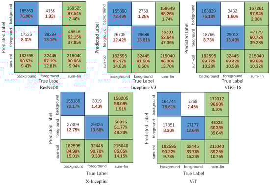
Figure 6.
Predict the confusion matrix on test set of pixels’ patches.
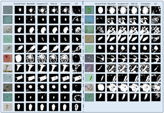
Figure 7.
Reconstruct the pixel patch transparent image segmentation results. (The figure contains the original image, ground truth image and Resnet50, Inception-V3, VGG-16, Xception, ViT network model predicted segmentation results).
3.3.2. Comparison Experiment of Pixel-Level Segmentation
To compare the effect of path-level segmentation, we conducted extended experiments using pixel-level segmentation. We applied five networks for the comparative experiments: U-Net, U-Net++, SegNet, TransUnet, and Swin-UNet. We used these five networks to compare the performance of the CNN and ViT for pixel-level segmentation. U-Net, U-Net++, and SegNet stand for CNN network, Swin-UNet stands for transformer networks, and TransUnet stands for CNNs joining the transformer. Table 6 presents the outcome of the five model prediction metrics. We found that U-Net++ exhibited the highest segmentation performance overall, but also had the longest training time. U-Net exhibited the worst segmentation performance. The segmentation result of the vision transformer network (Swin-UNet) was second after that of U-Net++. The Jaccard and precision values were 71.26% and 85.00%, respectively, which were higher than those of the other network models. To compare the segmentation results more intuitively, we presented the pixel-level segmentation results in Figure 8. Clearly, the pixel-level segmentation results are better than those of the patch level. However, the patch-level segmentation effect was better for multiobject transparent microorganism images. Compared to the patch-level segmentation, the network model with a transformer structure (Swin-UNet) at the pixel level performed well, and the ViT was higher than the accuracy of the CNN model. However, in the patch-level experiment, the accuracy of the CNN was higher than that of ViT. It is shown in Figure 5 that the loss curve stability of Swin-UNet is significantly better than that of the other four models during training. The training loss stability of the ViT model was better than that of the CNN model. To reflect the training process of the model more intuitively, the Intersection-over-Union (IOU) curves of the five models on the training and validation sets in the pixel-level experiment is presented in Figure 9.
Table 6.
Segmentation performance of models of five-fold cross-validation experiment on the test set.
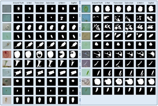
Figure 8.
Reconstruction of pixel-level segmentation results on transparent images of the test set. (The figure contains the original image, ground truth image and U-net, Trans-Unet, Swin-Unet, U-Net++, and SegNet network model predicted segmentation results).
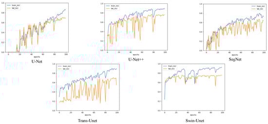
Figure 9.
A comparison of the image segmentation results of the IOU curves of deep learning on pixel-level training and validation sets.
3.3.3. Additional Experiment Based on EMDS-6 Dataset
To demonstrate the applicability of the models in our comparative experiments, we compared five models in pixel-level experiments on the EMDS-6 dataset. A partial EM sample of EMDS-6 is shown in Figure 10. EMDS-6 contains 840 EM’s microscopic images within 21 classes. We divided the dataset into training, validation, and test sets in a 1:1:2 ratio. We trained five models using the same parameters as those used in the EMDS-5 experiments. The performance metrics of the experimental results of the five models are presented in Table 7. We found that on EMDS-6, the pixel-level segmentation performance is consistent with the segmentation performance of EMDS-5. The segmentation performance of the U-Net, U-Net++, and Swin-Unet models was similar, and the segmentation accuracy was approximately 95%. SegNet exhibited the worst segmentation performance, with an accuracy of 91.21%. In addition, the number of images in EMDS-6 was twice that of EMDS-5; therefore, the model learns more EM information during training, leading to an overall improvement in the segmentation performance of the five models. The loss and IOU curves trained using the five models are shown in Figure 11 and Figure 12, respectively. We found that the loss and IOU curves trained by the five models were similar to the results in EMDS-5; therefore, the five models are suitable for comparison experiments. The segmentation results are shown in Figure 13.
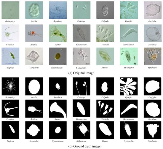
Figure 10.
Examples of the environmental microorganism image in EMDS-6. (a) is the original images of EMDS-6, each image contains one or more EM objects of the same species, and one image is selected for each species as a representative. (b) correspond to the real segmentation images of microorganisms in each image in the (a). The pixel value of the background part in the microorganism image is set to 0, and the foreground part is set to 1.
Table 7.
Segmentation performance of models of five-fold cross-validation experiment on the EMDS-6 test set.
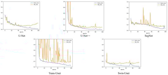
Figure 11.
A comparison of the image segmentation results of the loss and accuracy curves of deep learning on pixel-level training and validation set of EMDS-6.
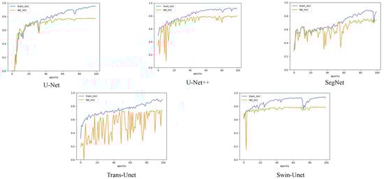
Figure 12.
A comparison of the image segmentation results of the IOU curves of deep learning on pixel-level training and validation sets of EMDS-6.
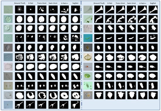
Figure 13.
Reconstruction of pixel-level segmentation results on transparent images the EMDS-6 test set. (The figure contains the original image, ground truth image and U-net, Trans-Unet, Swin-Unet, U-Net++, SegNet network model predicted segmentation results).
3.3.4. Experimental Environment
A comparative experiment was conducted using a local computer, with a running memory of 16 GB. The computer used the Win10 Professional operating system equipped with an 8 GB NVIDIA Quadro RTX 4000 GPU. In the patch-level experiment, the four CNN network models were imported from Keras version 2.3.1, and used TensorFlow 2.0.0 as the background. The experimental frameworks for ViT and pixel level were Pytorch 1.7.1 and Torchvision 8.0.2. Table 8 presents the model training and prediction time, and the size of the model during the experiment. From the perspective of model training time, the ViT model was much lower than CNN models, where the ViT training time was 13,992 s, and the Xception training time was the longest, 46,383 s. From the perspective of the model size, the minimum size of the ViT model was 31.2 M, and the maximum size of the ResNet50 model was 114 M. We calculated the times required for the five prediction models. The fastest prediction time for Inception-V3 was 583 s, and the prediction time for a single picture was 0.0027 s. The slowest time for ViT was 1308 s, and the prediction time of a single image was 0.0061 s.
Table 8.
A comparison of the classification results of five-fold cross-validation experiment on train and test sets of pixels patches. Train (Average training time), Test (Average test times) and Avg.p (Single picture prediction time) (In [s]).
3.4. In-Depth Analysis
In the predicted 215,040 patches, we compared the performance of five types of network classification: foreground and background. From Figure 6, Inception-V3 has the largest number of correct foregrounds under pixel patches, whereas ResNet50 has the largest number of correctly classified backgrounds. Furthermore, ViT network models misclassified foreground patches more than CNNs models. Consequently, the number of correctly classified foregrounds in the CNNs network was greater than that in the ViT network. Moreover, the ability of Swin-UNet to segment the foreground outperformed most models. Therefore, the ViT model was found as outstanding for low-transparency image recognition. Furthermore, in [32,36,49], on other datasets, the classification performance of the CNN model was better than that of the ViT network, and the training time of the ViT network model was less than that of the CNN model.
We found that the segmentation effect of the pixel level was higher than that of the patch level, but the segmentation result of the patch level can compensate for the loss of details of pixel-level segmentation. Therefore, we combined the patch-level and pixel-level segmentation results to obtain the optimal segmentation results. Figure 14 compares the GT, pixel-level, patch-level, and combined segmentation results. We set the segmentation region to a red mask and found that the combined results were significantly better than the single pixel-level or patch-level segmentation results.
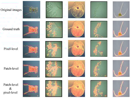
Figure 14.
Valid examples in EMDS-5 that fuse pixel-level segmentation and patch-level segmentation. From top to bottom, the images in each original image of EM, the EM represent GT image, pixel-level segmentation result, patch-level segmentation result, and combined result, respectively. (The red part in the figure is the segmentation result).
4. Discussion
This study investigates the patch-level and pixel-level segmentation performance of five deep learning models on the EMDS-5 [4]. The comparison results based on the evaluation indicators are listed in Table 4, Table 5, Table 6 and Table 8. In addition, to verify the generalization of the model, we used the same method to perform expansion experiments on the EMDS-6 dataset. The results are summarized in Table 4 and Figure 11, Figure 12 and Figure 13. To improve the reliability of the conclusion, all experimental results in this study were repeated five times, and then averaged for the final result [50].
In the patch-level segmentation experiments, the performance indicators of the five models were compared [49]. We found that all five deep learning models were better at classifying transparent image backgrounds than foregrounds. We can speculate that the foreground features of the transparent image are similar to those of the background, and all models had a strong ability to classify the background. Further, we compare the CNN and ViT models among the five models [14]. We found that ResNet50 [25] model had the highest segmentation performance; however, the ViT [31] model was better than the CNN model in terms of training time and model convergence speed. The ViT network has evident advantages in the time of training the model, and the time consumption is much less than that in other models. We can speculate that the ViT model may further expand its advantages when trained using more training data.
In the pixel-level segmentation experiment, we also conducted a comparative experiment between the CNN and ViT models. The model with the highest segmentation performance was U-Net++ [51]. Similarly, the Swin-UNet model [52], represented by the ViT model, had a better convergence speed than the CNN model. In addition, the accuracy of the Swin-UNet segmentation was better than that of U-Net, SegNet [53], and Trans-Unet [54].
The magnitude and index system of patch-level and pixel-level segmentation are different. Therefore, we cannot numerically compare the segmentation performance of the two groups of experiments. However, we made a full comparison between the patch-level and pixel-level visual segmentation results and fused the patch-level and pixel-level segmentation results to obtain a more complete segmentation result.
In computer vision tasks, image segmentation for multi-size EMs [5,55] and for weakly visible EMs [56,57] are introduced in recent years, where multi-scale CNN and pair-wise CNN methods are developed. However, the transparent EM image has not been developed and studied, so this paper used patch-level and pixel-level methods to segment transparent images, and a total of eight CNN and two ViT models were used to test the performance of the model. This study provides an analysis table of differences between the patch-level and pixel-level models. Our research and conclusions significantly reduce the workload of the researcher’s choice of experimental augmentation method. This reference is of great significance.
In this paper, we investigate deep learning methods for analyzing transparent EM images. In Section 2.1, we mentioned some existing techniques for analyzing transparent objects, and these techniques also have great potential in analyzing transparent EM images. For example, cleargrasp uses a deep convolutional network to infer surface normals, masks and occlusion boundaries on the surface of transparent objects. These outputs are then used to optimize the initial depth estimates of all transparent surfaces in the scene [17]. The leargrasp algorithm has great potential for transparent EM edge segmentation. In the industrial field, optical sensors are widely used to detect transparent objects by using the difference of light propagation rate through different media to determine transparent objects [19]. Optical sensors have potential value for transparent EM torso segmentation [20]. Meanwhile, the mean-shift algorithm and genetics algorithm also perform well in analyzing transparent objects, and we can also apply it to the segmentation of transparent EM blur and occluded locations [19,21]. The above methods of analyzing images have been proposed with the development of image processing technology, and these methods have the potential to contribute to the analysis of transparent EM images.
5. Conclusions and Future Work
In this study, we aimed to address the segmentation problems in transparent images by cropping the image into patches and classifying their foreground and background. We used CNNs and ViT deep learning methods to compare the patch-level and pixel-level performances of the transparent image segmentation. In segmenting transparent microorganism images, we found that the pixel-level generally outperforms the patch-level segmentation. However, the patch-level method works better in multiobject segmentation. Moreover, in the patch-level segmentation experiment, CNNs were better than the ViT models, but in the pixel-level experiment, the ViT model segmentation performed better than that of most CNNs. The smaller the patch pixel is, the more the regions perceived by the ViT model, and the stronger the ability to combine contextual information. Furthermore, the loss convergence and stability of the ViT model during training were better than those of the CNN model. In conclusion, the CNN and ViT models have more advantages in image classification. CNN is better at extracting the local features of images, whereas ViT is better at extracting the global features of images combined with contextual information. The ViT model has great potential for the future.
In the future, we plan to increase the amount of data to improve the stability of the comparisons. Meanwhile, images reconstructed by deep learning classification can be extended to the positioning, recognition, and detection of transparent images. We will further strengthen the applicability of these results.
Author Contributions
Conceptualization, C.L.; methodology, H.Y. and C.L.; software, H.Y.; validation, P.Z., A.C. and H.Y.; formal analysis, Y.T. and H.Y.; investigation, M.G. and T.J.; resources, X.Z.; data curation, C.L. and H.Y.; writing—original draft preparation, H.Y. and C.L.; writing—review and editing, C.L., J.Z., S.Q. and H.Y.; visualization, H.Y.; supervision, C.L.; project administration, C.L.; funding acquisition, C.L. and T.J. All authors have read and agreed to the published version of the manuscript.
Funding
National Natural Science Foundation of China (No.61806047) and Sichuan Science and Technology Plan (No. 2021YFH0069, 2021YFQ0057, 2022YFS056).
Institutional Review Board Statement
Not applicable.
Informed Consent Statement
Not applicable.
Data Availability Statement
Not applicable.
Acknowledgments
We thank Zixian Li and Guoxian Li for their important discussion.
Conflicts of Interest
The authors declare no conflict of interest.
References
- Liao, S.Y.; Aurelio, O.N.; Jan, K.; Zavada, J.; Stanbridge, E.J. Identification of the mn/ca9 protein as a reliable diagnostic biomarker of clear cell carcinoma of the kidney. Cancer Res. 1997, 57, 2827–2831. [Google Scholar] [CrossRef] [PubMed]
- Xue, D.; Zhou, X.; Li, C.; Yao, Y.; Rahaman, M.M.; Zhang, J.; Qi, S.; Sun, H. An application of transfer learning and ensemble learning techniques for cervical histopathology image classification. IEEE Access 2020, 8, 104603–104618. [Google Scholar] [CrossRef]
- Zhou, X.; Li, C.; Rahaman, M.M.; Yao, Y.; Ai, S.; Sun, C.; Wang, Q.; Zhang, Y.; Li, M.; Li, X.; et al. A comprehensive review for breast histopathology image analysis using classical and deep neural networks. IEEE Access 2020, 8, 90931–90956. [Google Scholar] [CrossRef]
- Li, Z.; Li, C.; Yao, Y.; Zhang, J.; Rahaman, M.M.; Xu, H.; Kulwa, F.; Lu, B.; Zhu, X.; Jiang, T. Emds-5: Environmental microorganism image dataset fifth version for multiple image analysis tasks. PLoS ONE 2021, 16, e0250631. [Google Scholar]
- Zhang, J.; Li, C.; Kosov, S.; Grzegorzek, M.; Shirahama, K.; Jiang, T.; Sun, C.; Li, Z.; Li, H. Lcu-net: A novel low-cost u-net for environmental microorganism image segmentation. Pattern Recognit. 2021, 115, 107885. [Google Scholar] [CrossRef]
- Kulwa, F.; Li, X.; Zhao, C.; Cai, B.; Xu, N.; Qi, S.; Chen, S.; Teng, Y. A state-of-the-art survey for microorganism image segmentation methods and future potential. IEEE Access 2019, 7, 100243–100269. [Google Scholar] [CrossRef]
- Khaing, M.P.; Masayuki, M. Transparent object detection using convolutional neural network. In Proceedings of the International Conference on Big Data Analysis and Deep Learning Applications, Miyazaki, Japan, 14–15 May 2018; Springer: Berlin/Heidelberg, Germany, 2018; pp. 86–93. [Google Scholar]
- Kosov, S.; Shirahama, K.; Li, C.; Grzegorzek, M. Environmental microorganism classification using conditional random fields and deep convolutional neural networks. Pattern Recognit. 2018, 77, 248–261. [Google Scholar] [CrossRef]
- Yoshua, B.; Yann, L.; Geoffrey, H. Deep learning. Nature 2015, 521, 436–444. [Google Scholar]
- Zhang, J.; Yang, K.; Constantinescu, A.; Peng, K.; Müller, K.; Stiefelhagen, R. Trans4trans: Efficient transformer for transparent object segmentation to help visually impaired people navigate in the real world. In Proceedings of the IEEE/CVF International Conference on Computer Vision, Montreal, QC, Canada, 10–17 October 2021; pp. 1760–1770. [Google Scholar]
- Yan, Z.; Zhan, Y.; Zhang, S.; Metaxas, D.; Zhou, X.S. Multi-instance multi-stage deep learning for medical image recognition. In Deep Learning for Medical Image Analysis; Elsevier: Amsterdam, The Netherlands, 2017; pp. 83–104. [Google Scholar]
- Ai, S.; Li, C.; Li, X.; Jiang, T.; Grzegorzek, M.; Sun, C.; Rahaman, M.M.; Zhang, J.; Yao, Y.; Li, H. A state-of-the-art review for gastric histopathology image analysis approaches and future development. BioMed Res. Int. 2021, 2021, 6671417. [Google Scholar] [CrossRef]
- Chen, H.; Li, C.; Li, X.; Rahaman, M.M.; Hu, W.; Li, Y.; Liu, W.; Sun, C.; Sun, H.; Huang, X.; et al. Il-mcam: An interactive learning and multi-channel attention mechanism-based weakly supervised colorectal histopathology image classification approach. Comput. Biol. Med. 2022, 143, 105265. [Google Scholar] [CrossRef]
- Dong, S.; Wang, P.; Abbas, K. A survey on deep learning and its applications. Comput. Sci. Rev. 2021, 40, 100379. [Google Scholar] [CrossRef]
- Raghu, M.; Unterthiner, T.; Kornblith, S.; Zhang, C.; Dosovitskiy, A. Do vision transformers see like convolutional neural networks? Adv. Neural Inf. Process. Syst. 2021, 34, 12116–12128. [Google Scholar]
- Zeng, A.; Yu, K.T.; Song, S.; Suo, D.; Walker, E.; Rodriguez, A.; Xiao, J. Multi-view self-supervised deep learning for 6d pose estimation in the amazon picking challenge. In Proceedings of the 2017 IEEE International Conference on Robotics and Automation (ICRA), Singapore, 29 May–3 June 2017; IEEE: Piscataway, NJ, USA, 2017; pp. 1383–1386. [Google Scholar]
- Sajjan, S.; Moore, M.; Pan, M.; Nagaraja, G.; Lee, J.; Zeng, A.; Song, S. Clear grasp: 3d shape estimation of transparent objects for manipulation. In Proceedings of the 2020 IEEE International Conference on Robotics and Automation (ICRA), Paris, France, 31 May–31 August 2020; IEEE: Piscataway, NJ, USA, 2020; pp. 3634–3642. [Google Scholar]
- Senturk, S.F.; Gulmez, H.K.; Gul, M.F.; Kirci, P. Detection and separation of transparent objects from recyclable materials with sensors. In Proceedings of the International Conference on Advanced Network Technologies and Intelligent Computing, Varanasi, India, 17–18 December 2021; Springer: Berlin/Heidelberg, Germany, 2021; pp. 73–81. [Google Scholar]
- Hata, S.; Saitoh, Y.; Kumamura, S.; Kaida, K. Shape extraction of transparent object using genetic algorithm. In Proceedings of the 13th International Conference on Pattern Recognition, Vienna, Austria, 25–29 August 1996; IEEE: Piscataway, NJ, USA, 1996; Volume 4, pp. 684–688. [Google Scholar]
- Xu, Y.; Nagahara, H.; Shimada, A.; Taniguchi, R.I. Transcut: Transparent object segmentation from a light-field image. In Proceedings of the IEEE International Conference on Computer Vision, Santiago, Chile, 7–13 December 2015; pp. 3442–3450. [Google Scholar]
- Guo, Y.; Xiong, Z.; Verbeek, F.J. An efficient and robust hybrid method for segmentation of zebrafish objects from bright-field microscope images. Mach. Vis. Appl. 2018, 29, 1211–1225. [Google Scholar] [CrossRef] [PubMed]
- Nasirahmadi, A.; Ashtiani, S.-H.M. Bag-of-feature model for sweet and bitter almond classification. Biosyst. Eng. 2017, 156, 51–60. [Google Scholar] [CrossRef]
- Xu, Y.; Maeno, K.; Nagahara, H.; Shimada, A.; Taniguchi, R.I. Light field distortion feature for transparent object classification. Comput. Vis. Image Underst. 2015, 139, 122–135. [Google Scholar] [CrossRef]
- Simonyan, K.; Zisserman, A. Very deep convolutional networks for large-scale image recognition. arXiv 2014, arXiv:1409.1556. [Google Scholar]
- He, K.; Zhang, X.; Ren, S.; Sun, J. Deep residual learning for image recognition. In Proceedings of the IEEE Conference on Computer Vision and Pattern Recognition, Las Vegas, NV, USA, 27–30 June 2016; pp. 770–778. [Google Scholar]
- Szegedy, C.; Liu, W.; Jia, Y.; Sermanet, P.; Reed, S.; Anguelov, D.; Erhan, D.; Vanhoucke, V.; Rabinovich, A. Going deeper with convolutions. In Proceedings of the IEEE Conference on Computer Vision and Pattern Recognition, Boston, MA, USA, 7–12 June 2015; pp. 1–9. [Google Scholar]
- Ioffe, S.; Szegedy, C. Batch normalization: Accelerating deep network training by reducing internal covariate shift. In Proceedings of the International Conference on Machine Learning, Lille, France, 6–11 July 2015; PMLR: New York City, NY, USA, 2015; pp. 448–456. [Google Scholar]
- Szegedy, C.; Vanhoucke, V.; Ioffe, S.; Shlens, J.; Wojna, Z. Rethinking the inception architecture for computer vision. In Proceedings of the IEEE Conference on Computer Vision and Pattern Recognition, Las Vegas, NV, USA, 27–30 June 2016; pp. 2818–2826. [Google Scholar]
- Chollet, F. Xception: Deep learning with depthwise separable convolutions. In Proceedings of the IEEE Conference on Computer Vision and Pattern Recognition, Honolulu, HI, USA, 21–26 July 2017; pp. 1251–1258. [Google Scholar]
- Ronneberger, O.; Fischer, P.; Brox, T. U-net: Convolutional networks for biomedical image segmentation. In Proceedings of the International Conference on Medical Image Computing and Computer-Assisted Intervention, Munich, Germany, 5–9 October 2015; Springer: Berlin/Heidelberg, Germany, 2015; pp. 234–241. [Google Scholar]
- Dosovitskiy, A.; Beyer, L.; Kolesnikov, A.; Weissenborn, D.; Zhai, X.; Unterthiner, T.; Dehghani, M.; Minderer, M.; Heigold, G.; Gelly, S.; et al. An image is worth 16x16 words: Transformers for image recognition at scale. arXiv 2020, arXiv:2010.11929. [Google Scholar]
- Chen, A.; Li, C.; Zou, S.; Rahaman, M.M.; Yao, Y.; Chen, H.; Yang, H.; Zhao, P.; Hu, W.; Liu, W.; et al. Svia dataset: A new dataset of microscopic videos and images for computer-aided sperm analysis. Biocybern. Biomed. Eng. 2022, 42, 204–214. [Google Scholar] [CrossRef]
- Li, C.; Chen, H.; Li, X.; Xu, N.; Hu, Z.; Xue, D.; Qi, S.; Ma, H.; Zhang, L.; Sun, H. A review for cervical histopathology image analysis using machine vision approaches. Artif. Intell. Rev. 2020, 53, 4821–4862. [Google Scholar] [CrossRef]
- Rahaman, M.M.; Li, C.; Wu, X.; Yao, Y.; Hu, Z.; Jiang, T.; Li, X.; Qi, S. A survey for cervical cytopathology image analysis using deep learning. IEEE Access 2020, 8, 61687–61710. [Google Scholar] [CrossRef]
- Rahaman, M.M.; Li, C.; Yao, Y.; Kulwa, F.; Wu, X.; Li, X.; Wang, Q. Deepcervix: A deep learning-based framework for the classification of cervical cells using hybrid deep feature fusion techniques. Comput. Biol. Med. 2021, 136, 104649. [Google Scholar] [CrossRef] [PubMed]
- Liu, W.; Li, C.; Rahaman, M.M.; Jiang, T.; Sun, H.; Wu, X.; Hu, W.; Chen, H.; Sun, C.; Yao, Y.; et al. Is the aspect ratio of cells important in deep learning? a robust comparison of deep learning methods for multi-scale cytopathology cell image classification: From convolutional neural networks to visual transformers. Comput. Biol. Med. 2021, 141, 105026. [Google Scholar] [CrossRef] [PubMed]
- Rahaman, M.M.; Li, C.; Yao, Y.; Kulwa, F.; Rahman, M.A.; Wang, Q.; Qi, S.; Kong, F.; Zhu, X.; Zhao, X. Identification of COVID-19 samples from chest x-ray images using deep learning: A comparison of transfer learning approaches. J. X-ray Sci. Technol. 2020, 28, 821–839. [Google Scholar] [CrossRef] [PubMed]
- Taha, A.A.; Hanbury, A. Metrics for evaluating 3d medical image segmentation: Analysis, selection, and tool. BMC Med. Imaging 2015, 15, 1–28. [Google Scholar] [CrossRef]
- Dimitri, G.M.; Agrawal, S.; Young, A.; Donnelly, J.; Liu, X.; Smielewski, P.; Hutchinson, P.; Czosnyka, M.; Lió, P.; Haubrich, C. A multiplex network approach for the analysis of intracranial pressure and heart rate data in traumatic brain injured patients. Appl. Netw. Sci. 2017, 2, 1–12. [Google Scholar] [CrossRef]
- Cicaloni, V.; Spiga, O.; Dimitri, G.M.; Maiocchi, R.; Millucci, L.; Giustarini, D.; Bernardini, G.; Bernini, A.; Marzocchi, B.; Braconi, D.; et al. Interactive alkaptonuria database: Investigating clinical data to improve patient care in a rare disease. FASEB J. 2019, 33, 12696–12703. [Google Scholar] [CrossRef]
- Kwekha-Rashid, A.S.; Abduljabbar, H.N.; Alhayani, B. Coronavirus disease (COVID-19) cases analysis using machine-learning applications. Appl. Nanosci. 2021, 1–13. [Google Scholar] [CrossRef] [PubMed]
- Zhao, P.; Li, C.; Rahaman, M.M.; Xu, H.; Yang, H.; Sun, H.; Jiang, T.; Grzegorzek, M. A comparative study of deep learning classification methods on a small environmental microorganism image dataset (emds-6): From convolutional neural networks to visual transformers. Front. Microbiol. 2022, 13, 792166. [Google Scholar] [CrossRef]
- Li, C. Content-Based Microscopic Image Analysis; Logos Verlag Berlin GmbH: Berlin, Germany, 2016; Volume 39. [Google Scholar]
- Wang, Y.; Ma, X.; Chen, Z.; Luo, Y.; Yi, J.; Bailey, J. Symmetric cross entropy for robust learning with noisy labels. In Proceedings of the IEEE/CVF International Conference on Computer Vision, Seoul, Korea, 27–28 October 2019; pp. 322–330. [Google Scholar]
- Wang, Y.; Yao, Q.; Kwok, J.T.; Ni, L.M. Generalizing from a few examples: A survey on few-shot learning. ACM Comput. Surv. 2020, 53, 1–34. [Google Scholar] [CrossRef]
- Deng, J.; Dong, W.; Socher, R.; Li, L.J.; Li, K.; Fei-Fei, L. Imagenet: A large-scale hierarchical image database. In Proceedings of the 2009 IEEE Conference on Computer Vision and Pattern Recognition, Miami, FL, USA, 20–25 June 2009; IEEE: Piscataway, NJ, USA, 2009; pp. 248–255. [Google Scholar]
- Zhu, H.; Jiang, H.; Li, S.; Li, H.; Pei, Y. A novel multispace image reconstruction method for pathological image classification based on structural information. BioMed Res. Int. 2019, 2019, 3530903. [Google Scholar] [CrossRef]
- Shin, H.C.; Roth, H.R.; Gao, M.; Lu, L.; Xu, Z.; Nogues, I.; Yao, J.; Mollura, D.; Summers, R.M. Deep convolutional neural networks for computer-aided detection: Cnn architectures, dataset characteristics and transfer learning. IEEE Trans. Med. Imaging 2016, 35, 1285–1298. [Google Scholar] [CrossRef]
- Zhao, P.; Li, C.; Rahaman, M.M.; Xu, H.; Ma, P.; Yang, H.; Sun, H.; Jiang, T.; Xu, N.; Grzegorzek, M. Emds-6: Environmental microorganism image dataset sixth version for image denoising, segmentation, feature extraction, classification, and detection method evaluation. Front. Microbiol. 2022, 1334. [Google Scholar] [CrossRef] [PubMed]
- Wong, T.-T.; Yeh, P.-Y. Reliable accuracy estimates from k-fold cross validation. IEEE Trans. Knowl. Data Eng. 2019, 32, 1586–1594. [Google Scholar] [CrossRef]
- Zhou, Z.; Siddiquee, M.M.R.; Tajbakhsh, N.; Liang, J. Unet++: Redesigning skip connections to exploit multiscale features in image segmentation. IEEE Trans. Med. Imaging 2019, 39, 1856–1867. [Google Scholar] [CrossRef] [PubMed]
- Cao, H.; Wang, Y.; Chen, J.; Jiang, D.; Zhang, X.; Tian, Q.; Wang, M. Swin-unet: Unet-like pure transformer for medical image segmentation. arXiv 2021, arXiv:2105.05537. [Google Scholar]
- Badrinarayanan, V.; Kendall, A.; Cipolla, R. Segnet: A deep convolutional encoder-decoder architecture for image segmentation. IEEE Trans. Pattern Anal. Mach. Intell. 2017, 39, 2481–2495. [Google Scholar] [CrossRef]
- Chen, J.; Lu, Y.; Yu, Q.; Luo, X.; Adeli, E.; Wang, Y.; Lu, L.; Yuille, A.L.; Zhou, Y. Transunet: Transformers make strong encoders for medical image segmentation. arXiv 2021, arXiv:2102.04306. [Google Scholar]
- Zhang, J.; Li, C.; Kulwa, F.; Zhao, X.; Sun, C.; Li, Z.; Jiang, T.; Li, H.; Qi, S. A multiscale cnn-crf framework for environmental microorganism image segmentation. BioMed Res. Int. 2020, 2020, 4621403. [Google Scholar] [CrossRef]
- Kulwa, F.; Li, C.; Zhang, J.; Shirahama, K.; Kosov, S.; Zhao, X.; Jiang, T.; Grzegorzek, M. A new pairwise deep learning feature for environmental microorganism image analysis. Environ. Sci. Pollut. Res. 2022, 29, 51909–51926. [Google Scholar] [CrossRef]
- Kulwa, F.; Li, C.; Grzegorzek, M.; Rahaman, M.M.; Shirahama, K.; Kosov, S. Segmentation of weakly visible environmental microorganism images using pair-wise deep learning features. arXiv 2022, arXiv:2208.14957. [Google Scholar] [CrossRef]
Publisher’s Note: MDPI stays neutral with regard to jurisdictional claims in published maps and institutional affiliations. |
© 2022 by the authors. Licensee MDPI, Basel, Switzerland. This article is an open access article distributed under the terms and conditions of the Creative Commons Attribution (CC BY) license (https://creativecommons.org/licenses/by/4.0/).