The Application of Fault-Tolerant Partition Resolvability in Cycle-Related Graphs

Abstract

The concept of metric-related parameters permeates all of graph theory and plays an important role in diverse networks, such as social networks, computer networks, biological networks and neural networks. The graph parameters include an incredible tool for analyzing the abstract structures of networks. An important metric-related parameter is the partition dimension of a graph holding auspicious applications in telecommunication, robot navigation and geographical routing protocols. A fault-tolerant resolving partition is a preference for the concept of a partition dimension. A system is fault-tolerant if failure of any single unit in the originally used chain is replaced by another chain of units not containing the faulty unit. Due to the optimal fault tolerance, cycle-related graphs have applications in network analysis, periodic scheduling and surface reconstruction. In this paper, it is shown that the partition dimension (PD) and fault-tolerant partition dimension (FTPD) of cycle-related graphs, including kayak paddle and flower graphs, are constant and free from the order of these graphs. More explicitly, the FTPD of kayak paddle and flower graphs is four, whereas the PD of flower graphs is three. Finally, an application of these parameters in a scenario of installing water reservoirs in a locality has also been furnished in order to verify our findings.

1. Introduction and Preliminaries

Graph theory is one of the significant territories in mathematics whose theoretical ideas have been highly utilized in research areas in computer science, such as data mining, image capturing and networking (see [1]). Utilization of graph theory has proffered significant stimulation in the development of the field, and graph theoretical concepts have led to many interesting real-life problems in the context of the Internet of Things and for routing, fraud detection, customer analysis and scheduling. Graph theory deals with various distance-related parameters, one of which is the metric dimension of graphs. The concept of the MD of a graph was proposed independently by Slater (see [2]) and Harary et al. (see [3]). A generalized version of the MD of a graph as a PD of a graph was proposed by Chartrand et al. (see [4]). The MD is based on the distances between the vertices, whereas the PD is based on the distances between the vertices and sets containing vertices. Both of these dimensions contribute in different areas, such as network discovery (see [5]), strategies for mastermind games (see [6]), image processing and game theory (see [3,7]).

Fault tolerance in resolvability preserves the resolvability status of the system even when one of the machines is lacking in performing its function. All the system developers are focusing on minimizing the probability of failure and maximizing the consistency of the system. Although the electronic systems have been carefully designed, with the passage of time, any of its units can fail to perform. It is compulsory for a fault-tolerant self-stable system that the faulty originally used chain will be replaced by a chain of units having fault-free units. Thus, a fault-tolerant design enables a system to perform its function even in the occurrence of faults.

Consider a connected graph ${\rm Y}$ of the order $\alpha$ with the vertex set $V\left({\rm Y}\right)$ and edge set $E\left({\rm Y}\right)$. If two vertices $\rho ,\tau \in V\left({\rm Y}\right)$, then the distance $d(\rho ,\tau )$ is the length of the shortest path between $\rho$ and $\tau$. The distance between a vertex $\tau$ and $Q\subseteq V\left({\rm Y}\right)$ is defined as $min\left\{d\right(\tau ,q\left)\right|q\in Q\}$ and is denoted by $d(\tau ,Q)$. For the vertex $\tau \in V\left({\rm Y}\right)$, $N\left(\tau \right)$ is the open neighborhood of $\tau$ in ${\rm Y}$ (i.e., $N\left(\tau \right)=\{y\in V({\rm Y}):y\mathrm{is}\mathrm{adjacent}\mathrm{to}\tau \}$, and the closed neighborhood of $\tau$ is $N\left[\tau \right]=N\left(\tau \right)\cup \left\{\tau \right\}$) (see [8]). For an ordered subset $\Omega =\{{\xi }_1,{\xi }_2,\dots ,{\xi }_{\lambda }\}$ of $V\left({\rm Y}\right)$, the representation of vertex $\tau$ with respect to $\Omega$ is the $\lambda$ vector $(d(\tau ,{\xi }_1),d(\tau ,{\xi }_2),\dots ,d(\tau ,{\xi }_{\lambda }))$, denoted by $r\left(\tau \right|\Omega )$. The subset $\Omega$ is called the resolving set(RS) of ${\rm Y}$ if the representation of $\tau$ with respect to $\Omega$ is distinct for all $\tau \in V\left({\rm Y}\right)$. The MD of ${\rm Y}$ is defined as $min\left\{\right|\Omega |$: $\Omega \mathrm{is}\mathrm{the}\mathrm{RS}\mathrm{of}{\rm Y}\}$ and is denoted by $\beta \left({\rm Y}\right)$. Bousquet et al. studied the MD on sparse graphs and its applications to zero forcing sets (see [9]). Ebrahimi et al. studied the MD of the complement of annihilator graphs associated with commutative rings (see [10]). Ahmed et al. computed the MD of a kayak paddle graph and cycle with a chord graph (see [11]). Imran et al. studied the MD problem of a flower graph (see [12]). The generalized version of the MD as a fault-tolerant metric dimension (FTMD) originated from Hernando et al. in 2008 (see [13]). If for every pair of different vertices $\rho ,\tau \in V\left({\rm Y}\right)$, then there exist at least two vertices $w_1,w_2\in \Omega$ such that $d(\rho ,w_l)\ne d(\tau ,w_l)$ for $l\in \{1,2\}$. Then, the RS $\Omega$ of $V\left({\rm Y}\right)$ is called fault-tolerant. The FTMD of ${\rm Y}$ is the least number of vertices in an RS $\Omega$ and is denoted by ${\beta }^{{}^{\prime }}\left({\rm Y}\right)$. Saha et al. discussed the FTMD of circulant graphs (see [14]). Raza et al. studied this graph parameter on certain inter-connection networks (see [15]).

For a given $\lambda$-ordered partition of vertices of a connected graph ${\rm Y}$, represented as $\aleph =\{{\aleph }_1,{\aleph }_2,\dots ,{\aleph }_{\lambda }\}$, the representation (distance code) of the vertex $\tau \in V\left({\rm Y}\right)$ is the vector $r\left(\tau \right|\aleph )=(d(\tau ,{\aleph }_1),d(\tau ,{\aleph }_2),\dots ,d(\tau ,{\aleph }_{\lambda }))$. The partition ℵ is called a resolving partition of ${\rm Y}$ if all the vertices of ${\rm Y}$ have unique representations (distance codes) with respect to ℵ. The minimum number of sets in the resolving partition for ${\rm Y}$ is known as the partition dimension (PD) of ${\rm Y}$ and is represented by $pd\left({\rm Y}\right)$. The $pd\left({\rm Y}\right)$ of various classes of connected graphs could be constant, bounded or unbounded. Chartrand et al. characterized the graphs with $pd\left({\rm Y}\right)$ 2 or $\alpha$ (see [4]). Sharp bounds for the PD of convex polytopes and flower graphs were provided by Chu et al. (see [16]). The PD of kayak paddle and cycle with chord graphs was discussed by Wei et al. (see [17]). Nithya et al. discussed the PD of honey comb, hexagonal cage and quartz networks (see [18]). Khali et al. provided the bounds on the PD of families of convex polytopes with pendent edges (see [19]). The PD of a thorn of fan graph and certain classes of series parallel graphs were computed by Mardhaningsih and Monica et al., respectively (see [20,21]).

The complexity in computing the $\beta \left({\rm Y}\right)$ of general graphs was investigated by Gary et al. and Khuller et al. (see [22,23]). As the PD problem is a generalized variant of a metric dimension, therefore, $pd\left({\rm Y}\right)$ is also an NP-hard problem.

The advancement of the concept of the $pd\left({\rm Y}\right)$ of a graph as a fault-tolerant partition dimension (FTPD) of graphs was proposed by Salman et al. (see [24]). For a given $\lambda$-ordered partition of vertices of a connected graph ${\rm Y}$, represented by $\aleph =\{{\aleph }_1,{\aleph }_2,\dots ,{\aleph }_{\lambda }\}$, the partition ℵ of ${\rm Y}$ is called a fault-tolerant resolving partition if every pair of distinct vertices $\rho ,\tau \in V\left({\rm Y}\right)$, $r\left(\rho \right|\aleph )$ and $r\left(\tau \right|\aleph )$ has representations (distance codes) which differ by at least two places. The FTPD of ${\rm Y}$ is defined as $min\left\{\right|\aleph |:\aleph \mathrm{is}\mathrm{fault}-\mathrm{tolerant}\mathrm{resolving}\mathrm{partition}\mathrm{of}{\rm Y}\}$ and is denoted by $\mathcal{P}\left({\rm Y}\right)$. The FTPDs of certain classes of graphs, namely homogeneous caterpillar (see [25]), cyclic network (see [26]) and tadpole and necklace graphs (see [27]), are discussed by Kamran et al. The FTPDs of toeplitz networks (see [28]), convex polytopes (see [29]) and circulant graphs having a $\{1,2\}$ connection set (see [30]) were discussed by Asim et al. For further studies on FTPDs, we refer to [31,32]. In this paper, we protract these studies by computing the FTPD of a kayak paddle graph and flower graph.

Chartrand et al. revealed the following results on $pd\left({\rm Y}\right)$”

Proposition 1

([4]). Let Υ be a graph. Then, the following hold:

(a) 

$pd\left({\rm Y}\right)\le \beta \left({\rm Y}\right)+1$;

(b) 

$pd\left({\rm Y}\right)=2$ iff ${\rm Y}=P_{\alpha }$, where $P_{\alpha }$ is a path.

Salman et al. introduced successive results for $\mathcal{P}\left({\rm Y}\right)$:

Proposition 2

([24]). Let Υ be a graph. Then, the following hold:

(a) 

For $\alpha \ge 3$, $3\le \mathcal{P}\left({\rm Y}\right)\le \alpha$;

(b) 

For $\alpha \ge 2$, $\mathcal{P}\left({\rm Y}\right)\le {\beta }^{{}^{\prime }}\left({\rm Y}\right)+1$.

In 2022, Asim et al. provided an important result for the FTPD of a graph in which the degree of any vertex was at least four. This result is given in the following lemma:

Lemma 1

([29]). Let Υ be a graph of the order $m\ge 5$. If Υ has a node of a degree of at least 4, then $\mathcal{P}\left({\rm Y}\right)\ge 4$.

The present paper is framed in this manner. Section 2 is concerned with the computation of the exact FTPD of a kayak paddle graph, and Section 3 concerns computing the FTPD of a class of flower graphs. Section 4 includes the application of an FTPD in a scenario of installing water reservoirs in a locality. Finally, in the concluding section, we close the paper by giving anticipatory remarks about future work.

2. FTPD of a Kayak Paddle Graph

We compute the FTPD of a kayak paddle graph in this section. The kayak paddle graph, denoted by $KP(l,t,s)$, has two cycles of lengths l and t connected by a path of a length s. The vertex set and edge set of the kayak paddle graph for $l\ge 3$, $t\ge 3$ and $s\ge 2$, are $V\left(KP(l,t,s)\right)=\{v_1,v_2,\dots ,v_{l+t+s-1}\}$ and $E\left(KP(l,t,s)\right)=\{v_j{v}_{j+1}:1\le j\le l-1\}\cup \left\{v_1{v}_l\right\}\cup \{v_j{v}_{j+1}:l+1\le j\le l+t-1\}\cup \left\{v_{l+1}{v}_{l+t}\right\}\cup \left\{v_1{v}_{l+t+1}\right\}\cup \{v_j{v}_{j+1}:l+t+1\le j\le l+t+s-2\}\cup \left\{v_{l+t+s-1}{v}_{l+1}\right\}$, respectively. The kayak paddle graph $KP(9,7,6)$ is shown in Figure 1. The $\beta \left(KP\right(l,t,s\left)\right)$ was computed in [11]:

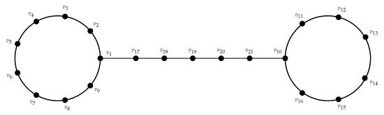
Figure 1. Kayak paddle graph $KP(9,7,6)$.

Lemma 2

([11]). For $l\ge 3$, $t\ge 3$ and $s\ge 2$, $\beta \left(KP\right(l,t,s\left)\right)=2$.

The $pd\left(KP\right(l,t,s\left)\right)$ was computed in [17]:

Lemma 3

([17]). For $l\ge 3$, $t\ge 3$ and $s\ge 2$, $pd\left(KP\right(l,t,s\left)\right)=3$.

The ensuing theorem will allow us to compute $\mathcal{P}\left(KP\right(l,t,s\left)\right)$ of the kayak paddle graph:

Theorem 1.

For $l\ge 3$, $t\ge 3$ and $s\ge 2$, $\mathcal{P}\left(KP\right(l,t,s\left)\right)=4$.

Proof. 

Let $\aleph =\{{\aleph }_1,{\aleph }_2,{\aleph }_3,{\aleph }_4\}$ be a partition set of $V\left(KP\right(l,t,s\left)\right)$. Take ${\aleph }_1=\{v_i:1\le i\le l-2,v_j:l+1\le j\le l+t-2\}$, ${\aleph }_2=\{v_{l-1},v_{l+t-1},v_j:l+t+1\le j\le l+t+s-1\}$, ${\aleph }_3=\left\{v_l\right\}$ and ${\aleph }_4=\left\{v_{l+t}\right\}$. The $r\left(v\right|\aleph )$ of the vertices of $KP(l,t,s)$ are shown in Table 1, Table 2, Table 3, Table 4, Table 5 and Table 6.

Table 1. Distance codes of $V\left(KP\right(l,t,s\left)\right)$ with respect to ℵ for $l=2ϵ$, where $ϵ\ge 2$, and $t=2b$, where $b\ge 2$.

Distance of Vertex	$\mathbf{From}{\mathit{\aleph }}_1$	$\mathbf{From}{\mathit{\aleph }}_2$	$\mathbf{From}{\mathit{\aleph }}_3$	$\mathbf{From}{\mathit{\aleph }}_4$
$v_r(1\le r\le ϵ-1)$	0	r	r	$s+r$
$v_{ϵ}$	0	$ϵ-1$	$ϵ$	$s+ϵ$
$v_{2ϵ-r-1}(1\le r\le ϵ-2)$	0	r	$r+1$	$s+r+3$
$v_{2ϵ-1}$	1	0	1	$s+3$
$v_{2ϵ}$	1	1	0	$s+2$
$v_{2ϵ+r}(1\le r\le b-1)$	0	r	$s+r$	r
$v_{2ϵ+b}$	0	$b-1$	$b+s$	b
$v_{l+t-r-1}(1\le r\le b-2)$	0	r	$s+r+3$	$r+1$
$v_{l+t-1}$	1	0	$s+3$	1
$v_{l+t}$	1	1	$s+2$	0
$v_{l+t+r}(1\le r\le \lfloor \frac{s}{2}\rfloor )$	r	0	$r+1$	$s-r+1$
$v_{l+t+s-r}(1\le r\le \lceil \frac{s}{2}\rceil -1)$	r	0	$s-r+1$	$r+1$

Table 2. Distance codes of $V\left(KP\right(l,t,s\left)\right)$ with respect to ℵ for $l=3$ and $t=3$.

Distance of Vertex	$\mathbf{From}{\mathit{\aleph }}_1$	$\mathbf{From}{\mathit{\aleph }}_2$	$\mathbf{From}{\mathit{\aleph }}_3$	$\mathbf{From}{\mathit{\aleph }}_4$
$v_1$	0	1	1	$s+1$
$v_2$	1	0	1	$s+2$
$v_3$	1	1	0	$s+2$
$v_4$	0	1	$s+1$	1
$v_5$	1	0	$s+2$	1
$v_6$	1	1	$s+2$	0
$v_{l+t+r}(1\le r\le \lfloor \frac{s}{2}\rfloor )$	r	0	$r+1$	$s-r+1$
$v_{l+t+s-r}(1\le r\le \lceil \frac{s}{2}\rceil -1)$	r	0	$s-r+1$	$r+1$

Table 3. Distance codes of $V\left(KP\right(l,t,s\left)\right)$ with respect to ℵ for $l=2ϵ+1$ when $ϵ\ge 2$ and $t=3$.

Distance of Vertex	$\mathbf{From}{\mathit{\aleph }}_1$	$\mathbf{From}{\mathit{\aleph }}_2$	$\mathbf{From}{\mathit{\aleph }}_3$	$\mathbf{From}{\mathit{\aleph }}_4$
$v_r(1\le r\le ϵ)$	0	r	r	$s+r$
$v_{ϵ+1}$	0	$ϵ-1$	$ϵ$	$s+ϵ+1$
$v_{2ϵ-r}(1\le r\le ϵ-2)$	0	r	$r+1$	$s+r+3$
$v_{2ϵ}$	1	0	1	$s+3$
$v_{2ϵ+1}$	1	1	0	$s+2$
$v_{2ϵ+2}$	0	1	$s+1$	1
$v_{l+t-1}$	1	0	$s+2$	1
$v_{l+t}$	1	1	$s+2$	0
$v_{l+t+r}(1\le r\le \lfloor \frac{s}{2}\rfloor )$	r	0	$r+1$	$s-r+1$
$v_{l+t+s-r}(1\le r\le \lceil \frac{s}{2}\rceil -1)$	r	0	$s-r+1$	$r+1$

Table 4. Distance codes of $V\left(KP\right(l,t,s\left)\right)$ with respect to ℵ for $l=2ϵ+1$, where $ϵ\ge 2$, and $t=2b+1$, where $b\ge 2$.

Distance of Vertex	$\mathbf{From}{\mathit{\aleph }}_1$	$\mathbf{From}{\mathit{\aleph }}_2$	$\mathbf{From}{\mathit{\aleph }}_3$	$\mathbf{From}{\mathit{\aleph }}_4$
$v_r(1\le r\le ϵ)$	0	r	r	$s+r$
$v_{ϵ+1}$	0	$ϵ-1$	$ϵ$	$s+ϵ+1$
$v_{2ϵ-r}(1\le r\le ϵ-2)$	0	r	$r+1$	$s+r+3$
$v_{2ϵ}$	1	0	1	$s+3$
$v_{2ϵ+1}$	1	1	0	$s+2$
$v_{2ϵ+r+1}(1\le r\le b)$	0	r	$s+r$	r
$v_{2ϵ+b+2}$	0	$b-1$	$b+s+1$	b
$v_{l+t-r-1}(1\le r\le b-2)$	0	r	$s+r+3$	$r+1$
$v_{l+t-1}$	1	0	$s+3$	1
$v_{l+t}$	1	1	$s+2$	0
$v_{l+t+r}(1\le r\le \lfloor \frac{s}{2}\rfloor )$	r	0	$r+1$	$s-r+1$
$v_{l+t+s-r}(1\le r\le \lceil \frac{s}{2}\rceil -1)$	r	0	$s-r+1$	$r+1$

Table 5. Distance codes of $V\left(KP\right(l,t,s\left)\right)$ with respect to ℵ for $l=2ϵ$, where, $ϵ\ge 2$, and $t=3$.

Distance of Vertex	$\mathbf{From}{\mathit{\aleph }}_1$	$\mathbf{From}{\mathit{\aleph }}_2$	$\mathbf{From}{\mathit{\aleph }}_3$	$\mathbf{From}{\mathit{\aleph }}_4$
$v_r(1\le r\le ϵ-1)$	0	r	r	$s+r$
$v_{ϵ}$	0	$ϵ-1$	$ϵ$	$s+ϵ$
$v_{2ϵ-r-1}(1\le r\le ϵ-2)$	0	r	$r+1$	$s+r+3$
$v_{2ϵ-1}$	1	0	1	$s+3$
$v_{2ϵ}$	1	1	0	$s+2$
$v_{2ϵ+1}$	0	1	$s+1$	1
$v_{l+t-1}$	1	0	$s+2$	1
$v_{l+t}$	1	1	$s+2$	0
$v_{l+t+r}(1\le r\le \lfloor \frac{s}{2}\rfloor )$	r	0	$r+1$	$s-r+1$
$v_{l+t+s-r}(1\le r\le \lceil \frac{s}{2}\rceil -1)$	r	0	$s-r+1$	$r+1$

Table 6. Distance codes of $V\left(KP\right(l,t,s\left)\right)$ with respect to ℵ for $l=2ϵ$, where, $ϵ\ge 2$, and $t=2b+1$, where $b\ge 2$.

Distance of Vertex	$\mathbf{From}{\mathit{\aleph }}_1$	$\mathbf{From}{\mathit{\aleph }}_2$	$\mathbf{From}{\mathit{\aleph }}_3$	$\mathbf{From}{\mathit{\aleph }}_4$
$v_r(1\le r\le ϵ-1)$	0	r	r	$s+r$
$v_{ϵ}$	0	$ϵ-1$	$ϵ$	$s+ϵ$
$v_{2ϵ-r-1}(1\le r\le ϵ-2)$	0	r	$r+1$	$s+r+3$
$v_{2ϵ-1}$	1	0	1	$s+3$
$v_{2ϵ}$	1	1	0	$s+2$
$v_{2ϵ+r}(1\le r\le b)$	0	r	$s+r$	r
$v_{2ϵ+b+1}$	0	$b-1$	$b+s+1$	b
$v_{l+t-r-1}(1\le r\le b-2)$	0	r	$s+r+3$	$r+1$
$v_{l+t-1}$	1	0	$s+3$	1
$v_{l+t}$	1	1	$s+2$	0
$v_{l+t+r}(1\le r\le \lfloor \frac{s}{2}\rfloor )$	r	0	$r+1$	$s-r+1$
$v_{l+t+s-r}(1\le r\le \lceil \frac{s}{2}\rceil -1)$	r	0	$s-r+1$	$r+1$

It is apparent from Table 1, Table 2, Table 3, Table 4, Table 5 and Table 6 that ℵ is a fault-tolerant resolving partition set of $KP(l,t,s)$, and therefore, $\mathcal{P}\left(KP\right(l,t,s\left)\right)\le 4$.

Now, we establish that $\mathcal{P}\left(KP\right(l,t,s\left)\right)\ge 4$. For this, we exhibit that $\mathcal{P}\left(KP\right(l,t,s\left)\right)\ne 3$. For a contradiction, we estimate that $\aleph =\{{\aleph }_1,{\aleph }_2,{\aleph }_3\}$ is a fault-tolerant partition basis of $KP(l,t,s)$. As $v_1$ and $v_{l+1}$ are only vertices of a degree of three, without loss of generality, we assume that $v_1\in {\aleph }_1$ and $N\left(v_1\right)=\{v_2,v_l,v_{l+t+1}\}$. Suppose that $|{\aleph }_1|=1$ and $N\left(v_1\right)\subseteq {\aleph }_2\cup {\aleph }_3$, $|N\left(v_1\right)\cap {\aleph }_2|\ge 2$ or $|N\left(v_1\right)\cap {\aleph }_3|\ge 2$. Without loss of generality, we suppose that at least two vertices $a,b\in N\left(v_1\right)\cap {\aleph }_2$. As $r\left(a\right|\aleph )=(1,0,c_1)$ and $r\left(b\right|\aleph )=(1,0,c_2)$ are the same in two places, this is hence a contradiction. Now, we consider the subsequent cases by assuming that $|{\aleph }_1|\ge 2$ and $v_1\in {\aleph }_1$:

Case 1:

If $N\left(v_1\right)\cap {\aleph }_1=\{v_2,v_l,v_{l+t+1}\}$, then $r\left(v_1\right|\aleph )=(0,a_0,b_0)$, $r\left(v_2\right|\aleph )=(0,a_1,b_1)$, $r\left(v_l\right|\aleph )=(0,a_2,b_2)$ and $r\left(v_{l+t+1}\right|\aleph )=(0,a_3,b_3)$. As $a_0-1\le a_1,a_2,a_3\le a_0+1$, two vertices will have two identical coordinates in their identification, thus creating a contradiction.

Case 2:

If $N\left(v_1\right)\cap {\aleph }_1=\{v_2,v_l\}$, and one vertex $v_{l+t+1}\in {\aleph }_2$, then $r\left(v_1\right|\aleph )=(0,1,b_0)$, $r\left(v_2\right|\aleph )=(0,a_1,b_1)$, $r\left(v_l\right|\aleph )=(0,a_2,b_2)$ and $r\left(v_{l+t+1}\right|\aleph )=(1,0,b_3)$. Since $1\le a_1,a_2\le 2$, two vertices will have two identical coordinates, thus creating a contradiction.

Case 3:

If $N\left(v_1\right)\cap {\aleph }_1=\left\{v_2\right\}$, and two vertices $v_l,v_{l+t+1}\in {\aleph }_2$, then $r\left(v_1\right|\aleph )=(0,1,b_0)$, $r\left(v_2\right|\aleph )=(0,a_1,b_1)$, $r\left(v_l\right|\aleph )=(1,0,b_2)$ and $r\left(v_{l+t+1}\right|\aleph )=(1,0,b_3)$. Again, $r\left(v_l\right|\aleph )$ and $r\left(v_{l+t+1}\right|\aleph )$ are identical in two places, thus creating a contradiction.

Case 4:

If $N\left(v_1\right)\cap {\aleph }_1=\left\{v_2\right\}$, $v_l\in {\aleph }_2$ and $v_{l+t+1}\in {\aleph }_3$, then $r\left(v_1\right|\aleph )=(0,1,1)$. Hence, we have the following four cases:

Case 4(a):

At least one of l or t is 3, so without loss of generality, we have $l=3$. As $r\left(v_2\right|\aleph )=(0,1,2)$, having the first two coordinates being the same as $r\left(v_1\right|\aleph )$, therefore, it is against our assumption.

Case 4(b):

At least one of l or t is 4, so without loss of generality, we have $l=4$. Here, $N\left(v_2\right)=\{v_3,v_1\}$, and let $v_3\in {\aleph }_1$. It can be seen that $r\left(v_2\right|\aleph )=(0,2,2)$ and $r\left(v_3\right|\aleph )=(0,1,3)$. As $r\left(v_1\right|\aleph )$ and $r\left(v_3\right|\aleph )$ have the same first two coordinates, this negates our claim.

Case 4(c):

If at least one of l or t is 5, then without loss of generality, we have $l=5$. Here, $N\left(v_2\right)=\{v_3,v_1\},N\left(v_5\right)=\{v_4,v_1\}$ and $N\left(v_{l+t+1}\right)=\{v_{l+t+2},v_1\}$. Let $v_3\in {\aleph }_1$ and $v_4,v_{l+t+2},\in {\aleph }_2\cup {\aleph }_3$. Without loss of generality, we suppose that $v_4,v_{l+t+2}$ belong to ${\aleph }_2$. Here, $r\left(v_2\right|\aleph )=(0,2,2)$ and $r\left(v_3\right|\aleph )=(0,1,d_1)$. As $r\left(v_1\right|\aleph )$ and $r\left(v_3\right|\aleph )$ have the same first two coordinates, this negates our claim. Now, if $v_4\in {\aleph }_2$ and $v_{l+t+2}\in {\aleph }_3$, then $r\left(v_3\right|\aleph )=(0,1,d_2)$. As $r\left(v_1\right|\aleph )$ and $r\left(v_3\right|\aleph )$ have their first two coordinates as identical, this opposes our claim. Now, if $v_{l+t+2}\in {\aleph }_2$ and $v_4\in {\aleph }_3$, then $r\left(v_l\right|\aleph )=(1,0,1)$ and $r\left(v_{l+t+2}\right|\aleph )=(d_3,0,1)$. As $r\left(v_1\right|\aleph )$ and $r\left(v_{l+t+2}\right|\aleph )$ have the same last two coordinates, which negates our claim.

Case 4(d):

Now, for $l\ge 6$ and $t\ge 6$, consider $N\left(v_2\right)=\{v_3,v_1\}$, $N\left(v_l\right)=\{v_{l-1},v_1\}$ and $N\left(v_{l+t+1}\right)=\{v_{l+t+2},v_1\}$. Let $v_3\in {\aleph }_1$ and $v_{l-1},v_{l+t+2}\in {\aleph }_2\cup {\aleph }_3$. Without loss of generality, we assume that $v_{l-1},v_{l+t+2}\in {\aleph }_2$. Here, $r\left(v_l\right|\aleph )=(1,0,2)$, $r\left(v_{l-1}\right|\aleph )=(a_0,0,c_1)$ and $r\left(v_{l+t+2}\right|\aleph )=(a_1,0,1)$. Since $1\le a_0,a_1\le 2$, then two vertices will have two identical coordinates, which contradicts the claim. Now, if $v_{l+t+2}\in {\aleph }_2$ and $v_{l-1}\in {\aleph }_3$, then $r\left(v_l\right|\aleph )=(1,0,1)$ and $r\left(v_{l+t+2}\right|\aleph )=(a_2,0,1)$. As $r\left(v_l\right|\aleph )$ and $r\left(v_{l+t+2}\right|\aleph )$ have the same last two coordinates, this negates our claim. If $v_{l-1}\in {\aleph }_2$ and $v_{l+t+2}\in {\aleph }_3$, then $N\left(v_{l-1}\right)=\{v_l,v_{l-2}\}$. Consider $v_{l-2}\in {\aleph }_1$ such that $r\left(v_l\right|\aleph )=(1,0,2)$ and $r\left(v_{l-1}\right|\aleph )=(1,0,a_3)$. As $r\left(v_l\right|\aleph )$ and $r\left(v_{l-1}\right|\aleph )$ have their first two coordinates as identical, this opposes our claim.

Case 5:

If $N\left(v_1\right)\cap {\aleph }_1=\varnothing$, and all the three vertices $v_2,v_l,v_{l+t+1}\in {\aleph }_2$, then $r\left(v_1\right|\aleph )=(0,1,b_0)$, $r\left(v_2\right|\aleph )=(1,0,b_1)$, $r\left(v_l\right|\aleph )=(1,0,b_2)$ and $r\left(v_{l+t+1}\right|\aleph )=(1,0,b_3)$. Again, $r\left(v_2\right|\aleph )$, $r\left(v_l\right|\aleph )$ and $r\left(v_{l+t+1}\right|\aleph )$ have two identical coordinates, thus forming a contradiction.

Case 6:

If $N\left(v_1\right)\cap {\aleph }_1=\varnothing$ and there are two vertices $v_2,v_l\in {\aleph }_2$ and one vertex $v_{l+t+1}\in {\aleph }_3$, then $r\left(v_1\right|\aleph )=(0,1,1)$, $r\left(v_2\right|\aleph )=(1,0,b_0)$ and $r\left(v_l\right|\aleph )=(1,0,b_1)$. Again, $r\left(v_2\right|\aleph )$ and $r\left(v_l\right|\aleph )$ have two identical coordinates, thus forming a contradiction.

It follows from the above discussion that $\mathcal{P}\left(KP\right(l,t,s\left)\right)\ge 4$. We end up with this conclusion by relating both inequalities, so $\mathcal{P}\left(KP\right(l,t,s\left)\right)=4$ completes the proof. □

3. FTPD of the Flower Graph

We compute the PD and FTPD of a class of flower graph in this section. A flower graph denoted by $f_{\alpha \times q}$ has $\alpha (q-1)$ vertices and $\alpha q$ edges. An $\alpha$ cycle is formed by the $\alpha$ vertices, and q cycles around the $\alpha$ cycle are formed by $\alpha$ sets of $q-2$ vertices. Each q cycle intersects the $\alpha$ cycle uniquely on a single edge. The q cycles and $\alpha$ cycle are called the petals and center of the flower graph, respectively. The degree of vertices of the center and of all other vertices are four and two, respectively. Consider a class of a flower graph for $q=3$, denoted by $f_{\alpha \times 3}$. The vertices of the center of $f_{\alpha \times 3}$ are denoted by $v_1,v_2,\dots ,v_{\alpha }$, and the vertices of the petals are denoted by $v_{\alpha +1},v_{\alpha +2},\dots ,v_{2\alpha }$. The set $\{v_1,v_2,\dots ,v_{2\alpha }\}$ is a vertex set, and the set $\{v_i{v}_{i+1},1\le i\le \alpha -1\}\cup \left\{v_1{v}_{\alpha }\right\}\cup \left\{v_1{v}_{2\alpha }\right\}\cup \{v_i{v}_{\alpha +i},v_{i+1}{v}_{\alpha +i},1\le i\le \alpha -1\}\cup \{v_{\alpha },v_{2\alpha }\}$ is an edge set of the flower graph $f_{\alpha \times 3}$. Flower graph $f_{9\times 3}$ is given in Figure 2.

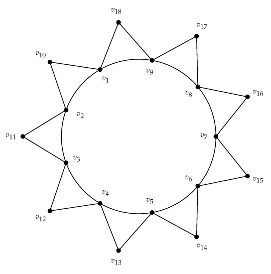
Figure 2. Flower graph $f_{9\times 3}$.

The $\beta \left(f_{\alpha \times 3}\right)$ was been computed in [12]:

Lemma 4

([12]). Let $f_{\alpha \times 3}$ be a flower graph. Then, we have

$$\beta \left(f_{\alpha \times 3}\right)=\left\{\begin{array}{cc}2,\hfill & if\alpha iseven;\hfill \\ 3,\hfill & otherwise\hfill \end{array}\right.$$

for every α ≥ 6

Lemma 5

([16]). Let $f_{\alpha \times 3}$ be a flower graph when α is odd. Then, $pd\left(f_{\alpha \times 3}\right)\le 4$.

The following theorem computes the exact partition dimension of $f_{\alpha \times 3}$:

Theorem 2.

Let $f_{\alpha \times 3}$ be a flower graph with $\alpha \ge 3$. Then, $pd\left(f_{\alpha \times 3}\right)=3$.

Proof. 

Suppose that $\aleph =\{{\aleph }_i:1\le i\le 3\}$ is a partition set of $V\left(f_{\alpha \times 3}\right)$. We consider the following cases:

Case (i):

When $\alpha$ is even for$\alpha \ge 4$.

It follows from Proposition 1(b) that $pd\left(f_{\alpha \times 3}\right)\ge 3$. Now, from Lemma 4 and Proposition 1(a), $pd\left(f_{\alpha \times 3}\right)\le 3$. Thus, $pd\left(f_{\alpha \times 3}\right)=3$.

Case (ii):

When$\alpha$ is odd for $\alpha \ge 3$.

Case ii(a):

When$\alpha =3$.

Consider ${\aleph }_1=\{v_i:1\le i\le 4\},{\aleph }_2=\left\{v_5\right\}$ and ${\aleph }_3=\left\{v_6\right\}$. It can easily be checked that ℵ is the resolving partition of $f_{\alpha \times 3}$.

Case ii(b):

When$\alpha =2ϵ+1$ for $ϵ\ge 2$. Consider ${\aleph }_1=\{v_i:1\le i\le \alpha +ϵ\}\cup \{v_i:\alpha +ϵ+2\le i\le 2\alpha -2\},{\aleph }_2=\left\{v_{\alpha +ϵ+1}\right\}$ and ${\aleph }_3=\{v_{2\alpha -1},v_{2\alpha }\}$. The distance codes of the vertices of $f_{\alpha \times 3}$ with respect to ℵ are given in Table 7.

Table 7. Distance codes of $V\left(f_{\alpha \times 3}\right)$ with respect to ℵ.

Distance of Vertex	$\mathbf{From}{\mathit{\aleph }}_1$	$\mathbf{From}{\mathit{\aleph }}_2$	$\mathbf{From}{\mathit{\aleph }}_3$
$v_r(1\le r\le ϵ)$	0	$ϵ-r+2$	r
$v_{ϵ+1}$	0	1	$ϵ$
$v_{ϵ+r+1}(1\le r\le ϵ-1)$	0	r	$ϵ-r$
$v_{2ϵ+1}$	0	$ϵ$	1
$v_{2ϵ+r}(2\le r\le ϵ+1)$	0	$ϵ-r+3$	r
$v_{3ϵ+2}$	1	0	$ϵ$
$v_{3ϵ+r+1}(2\le r\le ϵ-1)$	0	r	$ϵ-r+1$
$v_{4ϵ+r}(1\le r\le 2)$	1	$ϵ+r-1$	0

It is obvious from Table 7 that ℵ is a resolving partition of $f_{\alpha \times 3}$, and hence $pd\left(f_{\alpha \times 3}\right)\le 3$. Now, by Proposition 1(b), $f_{\alpha \times 3}$ is not a path graph, so it is not possible that the PD of $f_{\alpha \times 3}$ is two. Therefore, $pd\left(f_{\alpha \times 3}\right)\ge 3$, and from both acquired inequalities, $pd\left(f_{\alpha \times 3}\right)=3$, which concludes the proof. □

In the following theorem, we compute the $\mathcal{P}\left(f_{\alpha \times 3}\right)$:

Theorem 3.

Let $f_{\alpha \times 3}$ be a flower graph with $\alpha \ge 3$. Then, $\mathcal{P}\left(f_{\alpha \times 3}\right)=4$.

Proof. 

To prove that $\mathcal{P}\left(f_{\alpha \times 3}\right)=4$, we first show that $\mathcal{P}\left(f_{\alpha \times 3}\right)\le 4$. Let $\aleph =\{{\aleph }_e:1\le e\le 4\}$ be a partition set of $V\left(f_{\alpha \times 3}\right)$ for $\alpha \ge 3$.

Case (i):

When$\alpha =4$ and 5.

For $\alpha =4$, consider ${\aleph }_1=\{v_1,v_2,v_4,v_5\},{\aleph }_2=\{v_3,v_6\},{\aleph }_3=\left\{v_7\right\}$ and $L_4=\left\{v_8\right\}$, and for $\alpha =5$, consider ${\aleph }_1=\{v_1,v_2,v_6\},{\aleph }_2=\{v_3,v_4,v_5\},{\aleph }_3=\{v_7,v_8\}$ and ${\aleph }_4=\{v_9,v_{10}\}$. It is obvious that ℵ is a fault-tolerant resolving partition of $f_{\alpha \times 3}$.

Case (ii):

When$\alpha =3ϵ$ for $ϵ\ge 1$.

The partition representations of the vertices of $f_{\alpha \times 3}$ with respect to ${\aleph }_1=\{v_i:1\le i\le \alpha \},{\aleph }_2=\{v_i:\alpha +1\le i\le \alpha +ϵ\},{\aleph }_3=\{v_i:\alpha +ϵ+1\le i\le 2\alpha -ϵ\}$ and ${\aleph }_4=\{v_i:2\alpha -ϵ+1\le i\le 2\alpha \}$ are shown in Table 8.

Case (iii):

When$\alpha =3ϵ+1$ for $ϵ\ge 2$.

The partition representation of the vertices of $f_{\alpha \times 3}$, where ${\aleph }_1=\{v_i:1\le i\le \alpha \}\cup \{v_{\alpha +ϵ+1},v_{2\alpha -ϵ}\},{\aleph }_2=\{v_i:\alpha +1\le i\le \alpha +ϵ\},{\aleph }_3=\{v_i:\alpha +ϵ+2\le i\le 2\alpha -ϵ-1\}$ and ${\aleph }_4=\{v_i:2n-ϵ+1\le i\le 2n\}$, are shown in Table 9.

Case (iv):

When $\alpha =3ϵ+2$ for $ϵ\ge 2$.

The partition representation of vertices of $f_{\alpha \times 3}$, with respect to ${\aleph }_1=\{v_i:1\le i\le \alpha +1\},{\aleph }_2=\{v_i:\alpha +2\le i\le \alpha +ϵ+1\},{\aleph }_3=\{v_i:\alpha +ϵ+2\le i\le 2\alpha -ϵ\}$ and ${\aleph }_4=\{v_i:2\alpha -ϵ+1\le i\le 2\alpha \}$, are shown in Table 10.

Table 8. Distance codes of $V\left(f_{\alpha \times 3}\right)$ with respect to ℵ.

Distance of Vertex	$\mathbf{From}{\mathit{\aleph }}_1$	$\mathbf{From}{\mathit{\aleph }}_2$	$\mathbf{From}{\mathit{\aleph }}_3$	$\mathbf{From}{\mathit{\aleph }}_4$
$v_r(1\le r\le ϵ+1)$	0	1	$ϵ-r+2$	r
$v_{ϵ+r}(2\le r\le ϵ+1)$	0	r	1	$ϵ-r+2$
$v_{2ϵ+r}(2\le r\le ϵ)$	0	$ϵ-r+2$	r	1
$v_{3ϵ+r-1}(2\le r\le ϵ+1)$	1	0	$ϵ-r+3$	r
$v_{4ϵ+r-1}(2\le r\le ϵ+1)$	1	r	0	$ϵ-r+3$
$v_{5ϵ+r-1}(2\le r\le ϵ+1)$	1	$ϵ-r+3$	r	0

Table 8. Distance codes of $V\left(f_{\alpha \times 3}\right)$ with respect to ℵ.

Distance of Vertex	$\mathbf{From}{\mathit{\aleph }}_1$	$\mathbf{From}{\mathit{\aleph }}_2$	$\mathbf{From}{\mathit{\aleph }}_3$	$\mathbf{From}{\mathit{\aleph }}_4$
$v_r(1\le r\le ϵ+1)$	0	1	$ϵ-r+2$	r
$v_{ϵ+r}(2\le r\le ϵ+1)$	0	r	1	$ϵ-r+2$
$v_{2ϵ+r}(2\le r\le ϵ)$	0	$ϵ-r+2$	r	1
$v_{3ϵ+r-1}(2\le r\le ϵ+1)$	1	0	$ϵ-r+3$	r
$v_{4ϵ+r-1}(2\le r\le ϵ+1)$	1	r	0	$ϵ-r+3$
$v_{5ϵ+r-1}(2\le r\le ϵ+1)$	1	$ϵ-r+3$	r	0

Table 9. Distance codes of $V\left(f_{\alpha \times 3}\right)$ with respect to ℵ.

Distance of Vertex	$\mathbf{From}{\mathit{\aleph }}_1$	$\mathbf{From}{\mathit{\aleph }}_2$	$\mathbf{From}{\mathit{\aleph }}_3$	$\mathbf{From}{\mathit{\aleph }}_4$
$v_r(1\le r\le ϵ+1)$	0	1	$ϵ-r+3$	r
$v_{ϵ+r}(2\le r\le ϵ+1)$	0	r	1	$ϵ-r+3$
$v_{2ϵ+r}(2\le r\le ϵ+1)$	0	$ϵ-r+3$	r	1
$v_{3ϵ+r}(2\le r\le ϵ+1)$	1	0	$ϵ-r+4$	r
$v_{4ϵ+2}$	0	2	2	$ϵ+2$
$v_{4ϵ+r}(3\le r\le ϵ+1)$	1	r	0	$ϵ-r+4$
$v_{5ϵ+2}$	0	$ϵ+2$	2	2
$v_{5ϵ+r}(3\le r\le ϵ+2)$	1	$ϵ-r+4$	r	0

Table 9. Distance codes of $V\left(f_{\alpha \times 3}\right)$ with respect to ℵ.

Distance of Vertex	$\mathbf{From}{\mathit{\aleph }}_1$	$\mathbf{From}{\mathit{\aleph }}_2$	$\mathbf{From}{\mathit{\aleph }}_3$	$\mathbf{From}{\mathit{\aleph }}_4$
$v_r(1\le r\le ϵ+1)$	0	1	$ϵ-r+3$	r
$v_{ϵ+r}(2\le r\le ϵ+1)$	0	r	1	$ϵ-r+3$
$v_{2ϵ+r}(2\le r\le ϵ+1)$	0	$ϵ-r+3$	r	1
$v_{3ϵ+r}(2\le r\le ϵ+1)$	1	0	$ϵ-r+4$	r
$v_{4ϵ+2}$	0	2	2	$ϵ+2$
$v_{4ϵ+r}(3\le r\le ϵ+1)$	1	r	0	$ϵ-r+4$
$v_{5ϵ+2}$	0	$ϵ+2$	2	2
$v_{5ϵ+r}(3\le r\le ϵ+2)$	1	$ϵ-r+4$	r	0

Table 10. Distance codes of $V\left(f_{\alpha \times 3}\right)$ with respect to ℵ.

Distance of Vertex	$\mathbf{From}{\mathit{\aleph }}_1$	$\mathbf{From}{\mathit{\aleph }}_2$	$\mathbf{From}{\mathit{\aleph }}_3$	$\mathbf{From}{\mathit{\aleph }}_4$
$v_1$	0	2	$ϵ+1$	1
$v_r(2\le r\le ϵ+2)$	0	1	$ϵ-r+3$	r
$v_{ϵ+r+1}(2\le r\le ϵ+1)$	0	r	1	$ϵ-r+3$
$v_{2ϵ+r+2}(2\le r\le ϵ)$	0	$ϵ-r+3$	r	1
$v_{3ϵ+3}$	0	2	$ϵ+2$	2
$v_{3ϵ+r+1}(3\le r\le ϵ+2)$	1	0	$ϵ-r+4$	r
$v_{4ϵ+r+2}(2\le r\le ϵ+2)$	1	r	0	$ϵ-r+4$
$v_{5ϵ+r+3}(2\le r\le ϵ+1)$	1	$ϵ-r+4$	r	0

Table 10. Distance codes of $V\left(f_{\alpha \times 3}\right)$ with respect to ℵ.

Distance of Vertex	$\mathbf{From}{\mathit{\aleph }}_1$	$\mathbf{From}{\mathit{\aleph }}_2$	$\mathbf{From}{\mathit{\aleph }}_3$	$\mathbf{From}{\mathit{\aleph }}_4$
$v_1$	0	2	$ϵ+1$	1
$v_r(2\le r\le ϵ+2)$	0	1	$ϵ-r+3$	r
$v_{ϵ+r+1}(2\le r\le ϵ+1)$	0	r	1	$ϵ-r+3$
$v_{2ϵ+r+2}(2\le r\le ϵ)$	0	$ϵ-r+3$	r	1
$v_{3ϵ+3}$	0	2	$ϵ+2$	2
$v_{3ϵ+r+1}(3\le r\le ϵ+2)$	1	0	$ϵ-r+4$	r
$v_{4ϵ+r+2}(2\le r\le ϵ+2)$	1	r	0	$ϵ-r+4$
$v_{5ϵ+r+3}(2\le r\le ϵ+1)$	1	$ϵ-r+4$	r	0

It can be gleaned from Table 8, Table 9 and Table 10 that ℵ is a fault-tolerant resolving partition set of $f_{\alpha \times 3}$ such that $\mathcal{P}\left(f_{\alpha \times 3}\right)\le 4$. In addition, from Lemma 1, we have $\mathcal{P}\left(f_{\alpha \times 3}\right)\ge 4$. Thus, $\mathcal{P}\left(f_{\alpha \times 3}\right)=4$, which completes the proof. □

4. Application

Consider an example of water flow in a locality through a distribution network system using distribution reservoirs. The whole area is partitioned into a number of distribution sites, where distribution reservoirs are linked to the distribution sites with the help of distribution pipes. The aim is that the system should supply water to all the intended places optimally. The network distribution system could be affected by these factors:

1

If the reservoirs are located at a far distance from the place demanding water, then more operating power from the pumps should be used.

2

If the number of distribution sites increases, then the distribution time of the water also increases.

This scenario can be conveyed in terms of the PD as follows.

If in a distribution network system the area is partitioned into a number of distribution sites such that the distribution reservoirs supply water to all intended places, then the minimum number of reservoirs should be located in the minimum number of distribution sites so that each node uniquely recieves or supplies water, depending upon the minimum distance from the node to the partition set, and efficient utility of the network capacity be realized.

Consider a distribution network system in the form of $f_{9\times 3}$, whose nodes are arranged according to the partition sets given in Theorem 2. If one distribution reservoir is located in each of the distribution sites, as shown in Figure 3, then the network permits more flexible operation, and water reaches the given points such that a unique reservoir approaches a unique destination at the minimum distance. This explains the partition dimension of the graph.

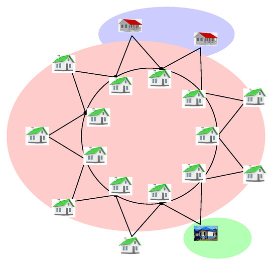
Figure 3. $f_{9\times 3}$ for partition dimension.

Furthermore, as the distribution network spreads geographically, and due to managing various network components, there is the possibility of failure of any node in a system. Thus, achieving fault tolerance is vital. Consider a distribution network system whose nodes are arranged according to the partition sets given in Theorem 3. If one-third of the number of vertices in each partition set are distribution reservoirs, as shown in Figure 4, then the service quality of an application will not degrade during the repair of any distribution reservoir of the system, and no consumer will be without a water supply. This explains the fault-tolerant partition dimension of the graph.

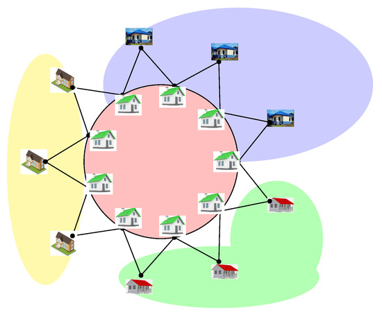
Figure 4. $f_{9\times 3}$ for fault-tolerant partition dimension.

5. Conclusions

In this paper, we computed $\mathcal{P}\left({\rm Y}\right)$ of two families of graphs. We conclude that for $l\ge 3$, $t\ge 3$ and $s\ge 2$, $\mathcal{P}\left(KP\right(l,t,s\left)\right)$ is 4, and $pd\left(f_{\alpha \times 3}\right)$ and $\mathcal{P}\left(f_{\alpha \times 3}\right)$ for $\alpha \ge 3$ are 3 and 4, respectively. For both families of graphs, $\mathcal{P}\left({\rm Y}\right)$ is constant and free from the order of graphs. Application of the FTPD in a scenario of installing water reservoirs in a locality was also provided, which verified our results. Computation of the PD and FTPD is NP-hard for general graphs. Due to this limitation, the problem of computing these parameters becomes interesting and challenging. In the future, it will be interesting to compute the FTPD of $f_{\alpha \times m}$, and also find applications of the FTPD in scenarios of transportation and scheduling.

References

- Meyer, A.R. Chapter 13, Communication networks. In Mathematics for Computer Science; MIT Open Learning Library: Cambridge, MA, USA, 2010; pp. 253–272. [Google Scholar]
- Slater, P.J. Leaves of trees. Proceeding of the 6th Southeastern Conf. Combinatorics, Graph Theory, and Computing. Congr. Numer. 1975, 14, 549–559. [Google Scholar]
- Harary, F.; Melter, R.A. On the metric dimension of a graph. Theory Comput. Syst. Ars Combinatoria 1976, 2, 191–195. [Google Scholar]
- Chartrand, G.; Salehi, E.; Zhang, P. The partition dimension of a graph. Aequ. Math. 2000, 59, 45–54. [Google Scholar] [CrossRef]
- Beerliová, Z.; Eberhard, F.; Erlebach, T.; Hall, A.; Hoffmann, M.; Mihalxaxk, M.; Ram, L.S. Network discovery and verification. IEEE J. Sel. Areas Commun. 2006, 24, 2168–2181. [Google Scholar] [CrossRef]
- Chvatal, V. Mastermind. Combinatorica 1983, 3, 325–329. [Google Scholar] [CrossRef]
- Melter, R.A.; Tomescu, I. Metric bases in digital geometry. Comput. Graph. Image Process. 1984, 25, 113–121. [Google Scholar] [CrossRef]
- Moreno, A.E. On the k-partition dimension of graphs. Theor. Compu. Sci. 2020, 806, 42–52. [Google Scholar] [CrossRef]
- Bousquet, N.; Deschamps, Q.; Parreau, A.; Pelayo, I. Metric dimension on sparse graphs and its applications to zero forcing sets. arXiv 2021, arXiv:2111.07845. [Google Scholar] [CrossRef]
- Ebrahimi, S.; Nikandish, R.; Tehranian, A.; Rasouli, H. Metric dimension of complement of annihilator graphs associated with commutative rings. In Applicable Algebra in Engineering, Communication and Computing; Springer: Berlin/Heidelberg, Germany, 2021. [Google Scholar] [CrossRef]
- Ahmad, A.; Bača, M.; Sultan, S. Computing the metric dimension of kayak paddle graph and cycles with chord. Proyecciones J. Math. 2020, 39, 287–300. [Google Scholar] [CrossRef]
- Imran, M.; Bashir, F.; Baig, A.; Bokhary, S.A.; Riasat, A.; Tomescu, I. On metric dimension of flower graphs fn×m and convex polytopes. Util. Math. 2013, 92, 389–409. [Google Scholar]
- Hernando, C.; Mora, M.; Slater, P.J.; Wood, D.R. Fault-tolerant metric dimension of graphs. In Proceedings of the International Conference on Convexity in Discrete Structures, Ramanujan Mathematical Society, Tiruchirappalli, India, 22 March–2 April 2008; pp. 81–85. [Google Scholar]
- Saha, L.; Lama, R.; Tiwary, K.; Das, K.C.; Shang, Y. Fault-tolerant metric dimension of circulant graphs. Mathematics 2022, 10, 124. [Google Scholar] [CrossRef]
- Raza, H.; Hayat, S.; Pan, X.F. On the fault-tolerant metric dimension of certain inter connection networks. J. Appl. Math. Comput. 2019, 60, 517–535. [Google Scholar] [CrossRef]
- Chu, Y.M.; Nadeem, M.F.; Azeem, M.; Siddiqui, M.K. On sharp bounds on partition dimension of convex polytopes. IEEE Access 2020, 8, 224781–224790. [Google Scholar] [CrossRef]
- Wei, C.; Nadeem, M.F.; Siddiqui, H.M.A.; Azeem, M.; Liu, J.B.; Khalil, A. On partition dimension of some cycle-related graphs. Math. Probl. Eng. 2021, 2021, 4046909. [Google Scholar] [CrossRef]
- Raj, R.N.; Raj, F.S. On the partition dimension of honey comb, hexagonal cage networks and quartz network. Ann. Rom. Soc. Cell Biol. 2021, 25, 2811–2817. [Google Scholar]
- Khali, A.; Husain, S.K.S.; Nadeem, M.F. On bounded partition dimension of different families of convex polytopes with pendant edges. AIMS Math. 2022, 7, 4405–4415. [Google Scholar] [CrossRef]
- Mardhaningsih, A. A note on the partition dimension of thorn of fan graph. Mantik 2019, 5, 45–49. [Google Scholar] [CrossRef]
- Monica, C.; Santhakumar, S.; Arockiaraj, M.; Liu, J.B. Partition dimension of certain classes of series parallel graphs. Theor. Compu. Sci. 2019, 778, 47–60. [Google Scholar] [CrossRef]
- Garey, M.R.; Johnson, D.S. Computers and Intractability, A Guide to the Theory of NP-Completeness; W.H. Freeman & Co. Ltd.: New York, NY, USA, 1979. [Google Scholar]
- Khuller, S.; Raghavachari, B.; Rosenfeld, A. Landmarks in graphs. Discret. Appl. Math. 1996, 70, 217–229. [Google Scholar] [CrossRef]
- Salman, M.; Javaid, I.; Chaudhry, M.; Shokat, S. Fault-tolerance in resolvability. Util. Math. 2009, 80, 263–275. [Google Scholar]
- Azhar, K.; Zafar, S.; Kashif, A. On fault-tolerant partition dimension of homogeneous caterpillar graphs. Math. Probl. Eng. 2021, 2021, 7282245. [Google Scholar] [CrossRef]
- Azhar, K.; Zafar, S.; Kashif, A.; Ojiema, M. Fault-tolerant partition resolvability of cyclic networks. J. Math. 2021, 2021, 7237168. [Google Scholar] [CrossRef]
- Azhar, K.; Zafar, S.; Kashif, A.; Zahid, Z. On fault-tolerant partition dimension of graphs. J. Intell. Fuzzy Syst. 2021, 4, 1129–1135. [Google Scholar] [CrossRef]
- Nadeem, A.; Kashif, A.; Aljaedi, A.; Zafar, S. On the fault tolerant partition resolvability of toeplitz networks. Math. Probl. Eng. 2022, 2022, 3429091. [Google Scholar] [CrossRef]
- Nadeem, A.; Kashif, A.; Bonyah, E.; Zafar, S. On the fault tolerant partition resolvability in convex polytopes. Math. Probl. Eng. 2022, 2022, 3238293. [Google Scholar] [CrossRef]
- Nadeem, A.; Kashif, A.; Zafar, S.; Zahid, Z. On 2-partition dimension of the circulant graphs. J. Intell. Fuzzy Syst. 2021, 40, 9493–9503. [Google Scholar] [CrossRef]
- Azhar, K.; Zafar, S.; Kashif, A.; Aljaedi, A.; Albalawi, U. Fault-tolerant partition resolvability in mesh related networks and applications. IEEE Access 2022, 10, 71521–71529. [Google Scholar] [CrossRef]
- Nadeem, A.; Kashif, A.; Zafar, S.; Zahid, Z. 2-partition resolvability of induced subgraphs of certain hydrocarbon nanotubes. Polycycl Aromat Comp. 2022, 1–11. [Google Scholar] [CrossRef]
Publisher’s Note: MDPI stays neutral with regard to jurisdictional claims in published maps and institutional affiliations. |
© 2022 by the authors. Licensee MDPI, Basel, Switzerland. This article is an open access article distributed under the terms and conditions of the Creative Commons Attribution (CC BY) license (https://creativecommons.org/licenses/by/4.0/).