


An Explainable and Lightweight Deep Convolutional Neural Network for Quality Detection of Green Coffee Beans


1
Department of Engineering Science, National Cheng Kung University, Tainan City 70101, Taiwan
2
Department of Computer Science and Information Engineering, National Llan University, Yilan County 26041, Taiwan
*
Authors to whom correspondence should be addressed.
Appl. Sci. 2022, 12(21), 10966; https://doi.org/10.3390/app122110966
Submission received: 18 September 2022
/
Revised: 25 October 2022
/
Accepted: 25 October 2022
/
Published: 29 October 2022
(This article belongs to the Topic Electronic Communications, IOT and Big Data)
Abstract
:In recent years, the demand for coffee has increased tremendously. During the production process, green coffee beans are traditionally screened manually for defective beans before they are packed into coffee bean packages; however, this method is not only time-consuming but also increases the rate of human error due to fatigue. Therefore, this paper proposed a lightweight deep convolutional neural network (LDCNN) for a quality detection system of green coffee beans, which combined depthwise separable convolution (DSC), squeeze-and-excite block (SE block), skip block, and other frameworks. To avoid the influence of low parameters of the lightweight model caused by the model training process, rectified Adam (RA), lookahead (LA), and gradient centralization (GC) were included to improve efficiency; the model was also put into the embedded system. Finally, the local interpretable model-agnostic explanations (LIME) model was employed to explain the predictions of the model. The experimental results indicated that the accuracy rate of the model could reach up to 98.38% and the F1 score could be as high as 98.24% when detecting the quality of green coffee beans. Hence, it can obtain higher accuracy, lower computing time, and lower parameters. Moreover, the interpretable model verified that the lightweight model in this work was reliable, providing the basis for screening personnel to understand the judgment through its interpretability, thereby improving the classification and prediction of the model.
1. Introduction
Coffee is a brewed beverage obtained by extracting in water the soluble components of the roasted pits of green coffee beans, which is not only flavorful but contains various levels of antioxidants and nutrients. Inoue et al. [1] conducted a prospective study with 90,452 subjects (including 43,109 men and 47,343 women) and found that hepatitis B and C virus-positive patients who consume one to two cups of coffee per day have a lower cirrhosis risk (relative risk = 50%) compared with that of those who almost never consumed coffee. Additionally, hepatitis B and C virus-positive patients who consume four cups of coffee per day have a lower cirrhosis and hepatitis risk (relative risk = 25%) compared with that of those who almost never consumed coffee. According to Loftfield et al. [2], drinking coffee is beneficial for heart health as caffeine can improve the cell processes in the blood vessels, especially the proteins in the cells of the elderly. When consumed in moderation, coffee can help prevent diseases like liver cancer, heart disease, dementia, or stroke. Hence, coffee has been one of the most widely consumed beverages in the world.
After collection, coffee beans should be handled quickly; otherwise, they will smell bad. Mature fruits will sink to the bottom of the tank after sun exposure and washing, while immature or broken beans tend to float on top. Green coffee beans are then picked out of the coffee fruit. Regardless of previous processing and selection, to remove defective beans, green coffee beans need to be manually selected; the selection process is a difficult one due to the brewing, mildew, brokerage, or worm damage during the peeling of beans. If defective beans are present before baking, chemical reactions may occur due to uneven heating, resulting in chemical toxins which can be harmful to health [3]. Therefore, to reduce labor costs, improve the quality of coffee, and increase profits, artificial intelligence (AI) has been introduced to pick out defective beans. The accurate and fast selection of defective beans using AI is an important automatic detection technology.
Many different algorithms have been applied to detect the quality of green coffee beans. For example, Santos et al. [4] employed spectroscopy to analyze the correlation between the quality of green coffee beans and near-infrared rays with a partial least square regression (PLS) model to predict defective coffee beans. However, the cost of detection instruments was too expensive; thus, it would be difficult to mass-produce. Oliveira et al. [5] put green coffee beans into a dark box without external light, captured the image through high-pixel RGB cameras, and converted RGB space colors to CIELAB. Later, they used a Bayesian classifier to improve coffee quality prediction. However, the test required a special environment, and the instrument cost was high. Arboleda et al. [6] extracted coffee bean features such as area of the bean, perimeter, equivalent diameter, and percentage of roundness, and employed an artificial neural network (ANN) and K nearest neighbor (KNN) to automatically categorize the coffee beans. Using ANN, the classification achieved score was 96.66%, while the classification score using KNN was at 84.12% [7]. Image-processing techniques were used to control coffee bean quality by extracting RGB color components based on 105 images of green coffee beans and 75 images of black beans with high accuracy. However, only 180 green coffee beans were tested [6,7]; this may cause poor stability during mass production due to the limited amount during testing. Hence, scholars began to improve stability through deep learning (DL). Pinto et al. [8] developed a convolutional neural network (CNN) that classified 13,000 green coffee beans images into six defect types. They sorted defective beans from 72.5% (broken bean) to 98.7% (black bean) accuracies, and the difference in the accuracy rate of detection in defective beans led to poor generalization of the model. Wang et al. [9] used a lightweight model with knowledge distillation (KD) and improved the accuracy of the training method to 91%, with the model parameters at only 256, 779. Huang et al. [10] extracted 1000 pleasant coffee beans and 1000 defective coffee beans and used image processing and data augmentation to deal with the data. Next, they applied YoloV3 to divide good and bad beans which had a recognition rate of 94.63%. Yang et al. [11] employed the CNN model based on KD, spatial-wise attention module (SAM), and SpinalNet [12] to achieve an accuracy rate of 96.54% on the F1 score. The recent progress in AI technology enables the labeling of data and the use of neural network design to allow the machine to automatically learn the data and the neural network to predict and make decisions based on the characteristics of the learned data. Although a deep convolutional neural network (DCNN) can accurately classify the images, it cannot be easily applied in embedded systems because its large Giga floating-point operations per second (GFLOPS) is the most popular method for model compression.
Quantization [13] and pruning technology are the most popular methods for model compression. Quantization converts the weight of a floating-point type into an integer type to reduce the amount of model parameters and computing while maintaining the accuracy of the model. In [14], a model architecture design that reduces the amount of model parameters and computation and also uses quantization technology and has a good compression effect while maintaining the accuracy of the model is proposed. However, there are many pruning-related methods, but they are rarely compared with other methods, or these methods have better results depending on the dataset. Therefore, in [15], the effect of different pruning on past research data is measured, as results show that pruning can sometimes improve the accuracy but the effect is usually not more stable than when using a better model architecture. Tang et al. [16] proposed an automatic pruning method, which does not need to set pruning standards and parameters. It is suitable for various neural network architectures and compares with other pruning methods that can effectively improve the compression ratio and reduce FLOPs. In [17], a network pruning method that can identify structural redundancy in CNNs and prune filters in selected layers with the most redundancy is proposed.
Generally, accuracy or evaluation indicators are very important for model efficiency when using DCNN for prediction and decision-making. Furthermore, explainable AI (XAI) will be lacking when DL technology is utilized. Hence, when using DL in models with high accuracy, the complexity may be high, while the correlation and hidden information cannot be explained through accuracy. Thus, scholars usually have difficulty understanding the correlation between input and output and how the model achieves its purpose. As a result, the uncertainty remains if people blindly believe in the model’s prediction. To solve this problem, XAI should be introduced to determine whether the prediction and evaluation of the decision making of the model based on certain characteristics are reasonable. Only in this way can the reliability of the model and quality detection be ensured in the future.
To deal with the above issues, this paper proposes a lightweight deep convolutional neural network (LDCNN) to detect the quality of green coffee beans. First, the features of defective coffee beans through RGB images were extracted, and the model was employed to classify the beans. Next, rectified Adam (RA), lookahead (LA), and gradient centralization (GC) were utilized to train the optimization methods to improve the accuracy of the model, enabling the model to operate in embedded systems.
2. Fundamental Knowledge
2.1. ResNet
2.2. MobileNetV3
MobileNetV3 [19] was put forward by Google in 2019 to deal with lightweight, whose bottleneck block can make the model lightweight and reduce GFLOPS using depthwise separable convolution (DSC), inverted residual block (IRB)[20], and squeeze-and-excite block (SE block)[21], as illustrated in Figure 2.
DSC comprises depthwise convolution (DC) and pointwise convolution (PC): the former aims to compress the channel of images, while the latter improves or reduces the dimensions of images of 1 × 1 pixel. Compared with an ordinary convolutional layer (CL), DSC can largely reduce GFLOPS without influencing performance; thus, it is now a widely used framework in lightweight models. The residual block of ResNet employs the general convolution layer to enhance dimensions and extract characteristics and connects two layers of large dimensions with longer GFLOPS. However, IRB connects two layers of small dimensions and extracts features of images through PC and DC, which can deliver high accuracy while reducing GFLOPS (see Figure 3).
As a lightweight attention module, the SE block, as shown in Figure 4, involves the relations among each channel and makes the model learn characteristics through the loss function. Thus, the weights of effective features increase while the weights of unimportant features decrease, allowing the model to learn varied importance levels of channel features to improve the accuracy.
2.3. Rectified Adam (RA)
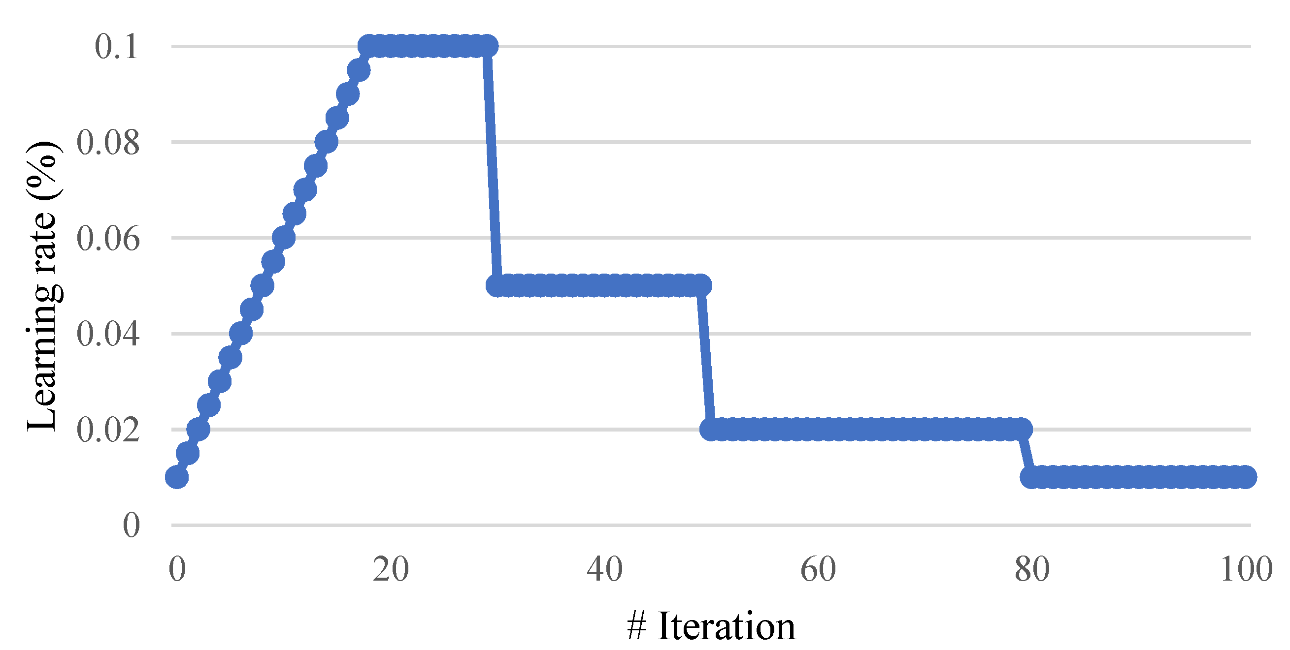
RA [22] employs both the Adam [23] optimizer and warm-up [24] to optimize the model. Unlike the general experimental algorithm that uses fixed intervals to reduce the learning rate, warm-up initially uses a rather low-learning-rate training model. Later, during the mechanism of warm-up, the learning rate increases gradually. When warm-up ends, the general process continues (see Figure 5). As previously suggested [23], since the initial value of model training is generated randomly and the model has no comprehension of the data, data loss will be large in the first epoch. Moreover, a large gradient causes large weight changes every time. Hence, it is easy to correct the feature distribution of data at the beginning of model training, while overfitting may occur frequently, or correction may be achieved only after multiple trainings. However, warm-up can address all those issues.
During the training of the model, RA can automatically correct the learning rate based on the degree of variation of the gradient and the number of samples. Therefore, with the quick convergence of Adam, the convergence can avoid the local minimum and reach the same results as the stochastic gradient descent (SGD) to make the training stable.
2.4. Lookahead (LA)
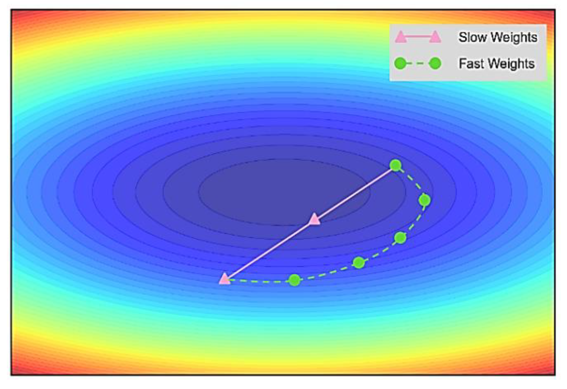
LA [25] initially generates fast and slow weights for the model separately and then updates fast weights during the training. The slow weights are updated towards the last fast weights after k batches. After each slow weight is updated, the fast weights are reset to the current slow weights’ value. Hence, the model’s weight does not easily converge at the local minimum. Figure 6 shows the contour map of the gradients. The LA optimization method can help the model continue to converge to the local minimum.
2.5. Gradient Centralization (GC)
Gradient descent is of great importance to effectively and efficiently train a DCNN, which can directly affect the model’s convergence speed and prediction accuracy. When the model becomes larger, the gradient descent becomes more difficult, causing issues like gradient vanishing, gradient exploding, or nonconvergence to affect the accuracy. To deal with this, GC [26] was presented to make the gradient descent smoother and to normalize the gradient before backward propagation, as described in Equation (1). GC operates directly on gradients by centralizing each column of convolutional layers and fully connected layers to have zero mean; the gradient is then subtracted from its mean value and sent back to continue the training of the model, as illustrated in Figure 7. Hence, the abnormal data will not affect the training process.
where Wi denotes the weight matrix of CL or FCL. The gradient is obtained through backward propagation of . After the calculation of mean value μ, average can be realized, and is gained through GC.
2.6. Local Interpretable Model-Agnostic Explanations (LIME)
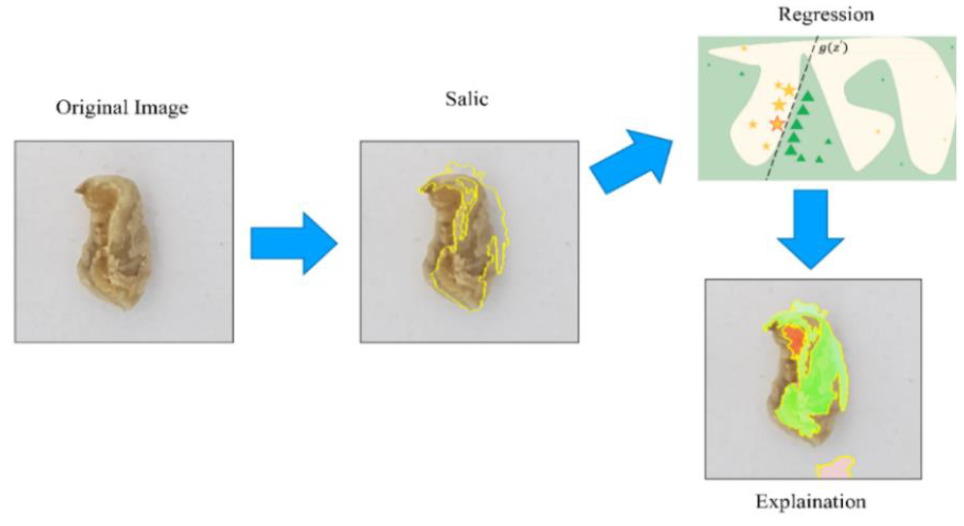
LIME [27], a local interpretable regression model, can provide the local area of the sample to find a simple and interpretable model when faced with complicated models. First, the images are separated into multiple sub-blocks; next, sub-blocks are randomly disturbed, and their predictions of complicated models are observed; later, after obtaining many samples of features, the local similarity is defined through regression, and the XAI is trained to explain and visualize complicated models as suggested in Equation (2).
Initially, sample is divided into several sub-blocks; then, sub-blocks are randomly disturbed to observe the predictions of the model f with high reviews. Next, a simple linear regression model g is trained to explain the predictions, and is used to measure the differences between the complex model and the interpretation model. refers to a measure of complexity to analyze and explain the judgment basis of the complex model for the image (Figure 8).
3. Proposed Methodology
The proposed methodology and experiment process is shown in Figure 9. The dataset and DA are described in the next section. In this section, image preprocessing and the training process of the proposed model are explained.
3.1. Image Preprocessing
The model should be lightweight to extract features of images and reduce noises and the size of input images. Hence, image preprocessing was carried out before inputting it into DCNN. To ensure that each input image was of the same size during training and validation, as minimizing the image size can reduce the parameters of the model and increase GFLOPS, image size was reduced from 400 × 400 × 3 to 224 × 224 × 3. Using bilinear interpolation, the image of the dataset was resized. In this paper, the RGB average value and standard deviation of the parameters set for image normalization (Figure 10) were the average value and standard deviations obtained from millions of images using ImageNet [28]. This is described in Equations (3) and (4).
3.2. Lightweight Deep Convolutional Neural Network (LDCNN)
The LDCNN proposed in this paper took an SE block as the backbone and used DSC to extract features of input images and adjust output dimensions. Figure 11 demonstrates the structure of the SE block. The image features went through the PC first to improve the dimensions, and pointwise features were extracted in the space. Next, image features between each pixel channel were extracted by DC and compressed using global average pooling (GAP). Then, the features were multiplied by input images through the ReLU activation function to expand. Therefore, high weights were enhanced while other weights were diminished, and the dimensions of output images were finally changed.
The LDCNN model in this study used the SE block as the backbone (Figure 12). Initially, the input image improved the dimensions of images through a single CL. Later, after undergoing the SE block twice, tiny features were extracted. Then, a skip block was employed to extract features through a skip connection. For instance, residual learning of ResNet can help the model avoid the difficulty of training deep networks due to weight degradation. Therefore, a skip block was added in this paper to improve the model’s accuracy. An SE block can extract channel-wise features of image features. However, after feature extraction, the features mainly focus on the correlation between image channels and channels, while feature extraction of global images is lacking. Hence, the model in this study additionally extracted features of the average pooling layer (APL) and CL as the skip block of the model. Two different features were added for classification, and GAP was used to connect CL and FCL on the tail structure of the model. Feature extraction was performed on global images, and the results were then classified.
Table 1 shows the model structure. As this study targets a lightweight model, the depth of the model was reduced, and a three-layer bottleneck block and ReLU activation function were adopted to minimize the GFLOPS and the parameters of the model. Furthermore, to maintain the model’s accuracy, the SE layer was used, and the dimensions of the images were increased. An H-swish (HS) activation function was adopted at both ends of the model structure to reduce GFLOPS and keep the accuracy of the model as opposed to ReLU. A 28 × 28 APL was used at the end to reduce the GFLOPS. By combining those models, we believe that high accuracy and a lightweight model could be realized.
To evaluate the efficiency of the model, fivefold cross-validation was adopted in the experiment to train and evaluate the model. The dataset was randomly divided into five groups, four of which contained 3701 images, and the remaining one included 3700 images. During the training process, one dataset was chosen while the others were used for training. After performing the experiment five times, the average evaluation results were calculated. Due to the limited parameters of the lightweight model and small GFLOPS, the model failed to extract complete features, which may have resulted in overfitting. To solve those issues, RA, LA, and GC were introduced in this lightweight model to optimize the learning rate strategy, weight, optimizer, and gradient. Finally, to evaluate the efficiency of LDCNN and predict reliability, except for calculating evaluation indicators, model size, parameters, GFLOPS, evaluation time, and comparing state of the art, this model was put into embedded systems. Moreover, this work adopted LIME to explain the predictions of LDCNN in model reliability.
4. Experimental Result
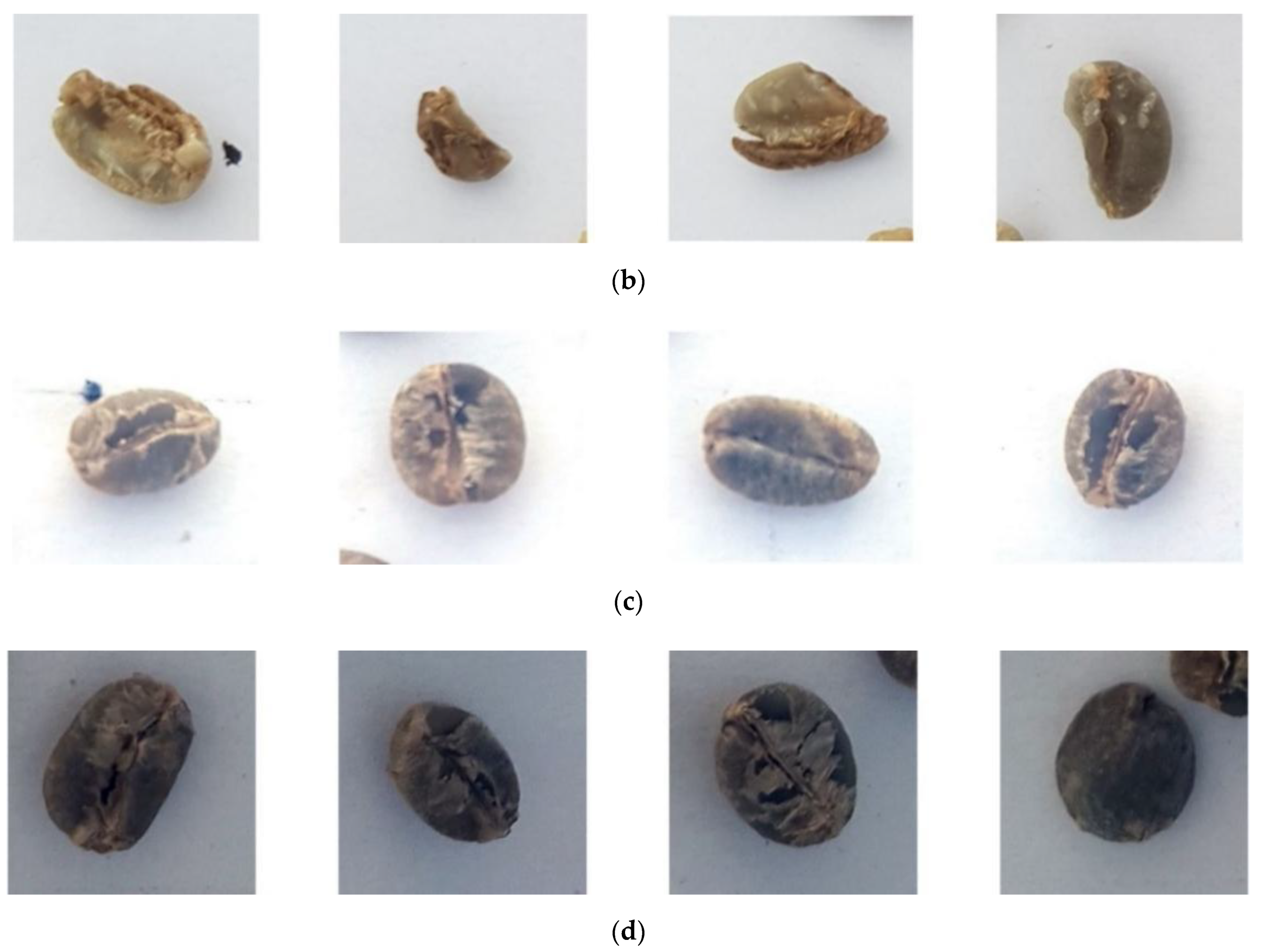
In this, we would like to introduce comparisons of the proposed model with previous related models. The green coffee bean dataset provided by a small optical sorter [29] included 4626 images that were 400 × 400 pixels. It consisted of 2149 good images and 2477 bad images; sample images are shown in Figure 13. The author collected the images of green coffee beans through high-speed cameras and conveyor belts and reduced the brightness of the shooting environment to minimize the shadows and centralize each image. Figure 13a,b shows good and bad images, respectively, while Figure 13c,d is images with adjusted brightness. In addition, the computer used for simulations was an AMD Ryzen™ 7 4800H CPU and GeForce GTX 1660 Ti GPU with 16GB DDR4 RAM. We implemented this research by using Python 3.8.11 and Pytorch 1.7.1, Pytorchvision 0.8.2, cudatookit 10.1, OpenCV 4.5.4 Library on a Windows 10 OS.
To achieve DA (including horizontal and vertical turning and 180° rotation) without any changes in shape, color, and background of images, the number of images was expanded from 4626 to 18,504 as the training dataset of this study. The image input model after DA helped improve the accuracy and generalization of the model.
4.1. The Influence of Image Normalization on Model
Image normalization means scaling the values of original images within an interval to extract the features and avoid the influence of abnormal values on the training results of the model. In this paper, an Adam optimizer was used, the learning rate was set at 0.001, batch size was 16, and 100 epochs were trained. Using the same validation method, we figured out that image normalization had significantly improved the accuracy of LDCNN as shown in Table 2.
4.2. Ablation Study of Training and Optimization in the Model
Cross-validation was employed to obtain evaluation indicators using the training dataset. As indicated in Table 3, the accuracy rate of the model was 98.38%, the precision rate was 98.60%, the recall rate was 97.89%, and the F1 score was 98.24%. The parameters were 149,842, the model size was 0.57 MB, GFLOPS was 0.05, and the computing time was 10.08 ms (see Table 4). The computing time is the average time of image preprocessing and model prediction. As shown, the various evaluation indicators of the model were of satisfactory accuracy while the model was kept lightweight. Afterwards, the training and optimization methods were employed to carry out the ablation study. Adam, cross-entropy loss function, and learning rate of 0.001 were used to evaluate and analyze the RA, LA, and GC methods.
Based on the experiment results, compared to when the Adam optimizer was used, the accuracy rate improved by 0.14%, the precision rate increased to 99.09%, and the recall rate was reduced by 1.80% when RA was employed. Therefore, the generalization ability of the RA model was low. When using GC, evaluation indicators of the model improved compared with those without optimization, indicating that GC effectively improved the detection rate of the model. On the contrary, when using LA, all the evaluation indicators were lower than those without optimization. Moreover, the evaluation indicators of LA-GC were lower than those of GC. While using the three methods simultaneously, the accuracy rate reached 98.38%, and F1 score achieved 98.24%. According to the results in Table 3, the Adam optimizer was not suitable for training with LA. Only when both RA and LA were used could the model’s accuracy be improved. When GC was the only one used, the recall index was the highest. Therefore, the three optimization methods to train the model simultaneously could obtain excellent stability and generalization.
Figure 14a,b shows the training process of LDCNN and the training process using three optimization and training methods, respectively. No obvious underfitting or overfitting occurred during both training processes. However, the accuracy sometimes dropped suddenly during the training, as the model generated random predictions due to rapid convergence and insufficient parameters. After adding the optimization method, the training stability significantly improved. Hence, the convergence should be stable to improve the accuracy, showing that the model could significantly improve the stability and generalization after combining the training method.
4.3. Evaluation Results of Interpretable Model
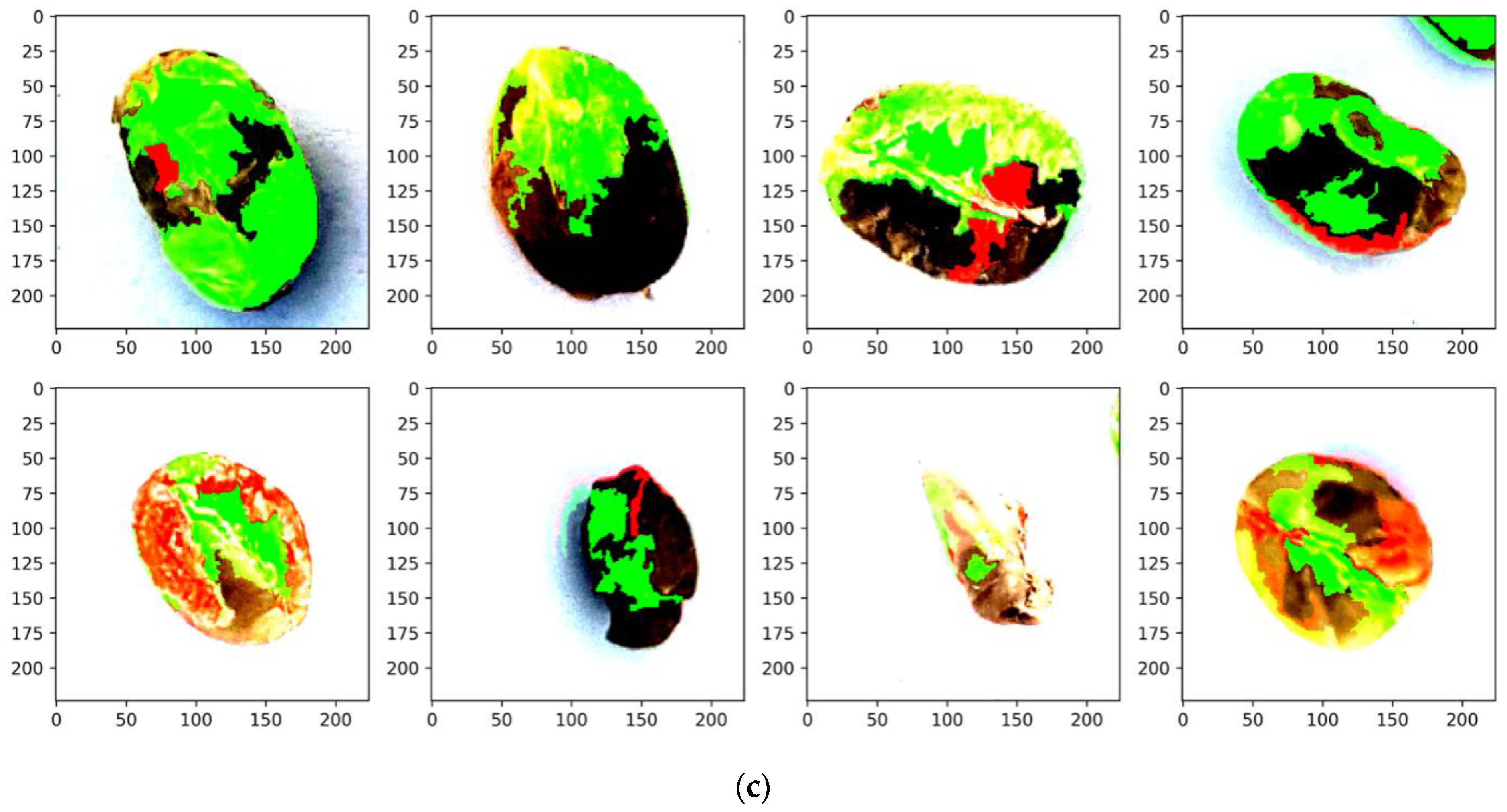
Figure 15a represents the original image of green coffee beans, and the upper and lower parts are good and bad coffee beans, respectively. Figure 15b,c is the visualization of the interpretation model prediction when the LDCNN optimization model went through LIME. The green block of coffee beans is the area favorable to the prediction results, and the red block is the unfavorable area. Based on Figure 15b, after XAI, the distribution of green areas may also exist in the surroundings of the coffee beans. It shows that the model took the background of coffee beans as the basis for judgment when predicting the quality of beans, and there was no obvious area that could be considered as the reference for judgment. Figure 15c, demonstrates that the favorable and unfavorable areas of beans could be revealed by predicting the area of the coffee beans.
To conclude, the prediction of the LDCNN optimization model was reliable, and the impact of image normalization on model training could also be understood after the image was visualized through LIME. Hence, the training could be optimized, or the abnormal data could be screened out from the dataset so the model could get better accuracy during the training process.
4.4. Comparison of Model Efficiency & Embedded System
To compare the models and training methods proposed in this paper, this experiment chose famous models, including ResNet [18], MobileNetV3 [19], EfficientNetV2 [30], and ShuffleNetV2 [31], to evaluate and compare with LDCNN. In this experiment, the same dataset was used to train each model. The Adam optimizer was employed, learning rate was set to 0.001, batch size was 16, and 100 epochs were trained. This study used the public dataset of green coffee beans, because most of the related research uses private datasets and is not public. In this work, the evaluation indicators of each model were tested, including accuracy, precision, recall, F1 score, parameter, model size, GFLOPs, and evaluation time, as shown in Table 4. We used the F1 score divided by eval time for evaluation. If the value was higher, the proposed model was the best in the green coffee bean identification task, as shown in Figure 16. As suggested in Table 4, in the quality detection of green coffee beans, the accuracy rate was better when LDCNN was used than when other models were utilized. However, the accuracy rate was quite low with the ResNet model compared with that with the other models; ResNet18 had an accuracy of only 89.66%, and ResNet 34 and ResNet 50 had decreased accuracy due to overfitting under increased CL.
Based on relevant research of public datasets [29], a lightweight model was proposed by Wang et al. [9] in which the ResNet18 model was trained as a teacher model through knowledge distillation (KD) to train the lightweight model. The accuracy rate of the lightweight model reached up to 91% with parameters of 256,779. As illustrated in Table 5, Yang et al. [11] put forward DSC, SAM, SpinalNet, and KD methods to train the model when the F1 score achieved 96.54%. Compared with LDCNN, the previous model [9] had higher accuracy and lower parameters since the latter took ResNet18 as the teacher model for training. Nevertheless, ResNet18 in this experiment was not the optimal model, resulting in a low accuracy rate of the lightweight model. In contrast to Yang et al. [11], the precision of LDCNN increased by 2.12%, recall was raised by 0.36%, and F1 score gained 1.74%. Finally, the LDCNN was placed on Raspberry Pi 4B to execute the green coffee bean quality detection system (see Table 6). The evaluation time included model building, image preprocessing, and image estimation time, which showed that LDCNN could achieve the task of real-time detection on the embedded system. The model was performed using Python programming language on Raspberry Pi 4B. The experiment used a 3701 verification dataset, and evaluation time was the time it took the model to predict 3701 images (including the preprocessing time). A total of 1226.57 s was used during the experiment when hardware acceleration method was not used. However, the image size of the verification dataset had been converted to 224 × 224 × 3 in numpy array format, so that the model could be executed on limited memory, and the implementation of the model on the embedded system.
5. Conclusions and Future Work
In this study, a new model for quality detection of green coffee beans, a LDCNN, was proposed, which combined DSC, SE block, skip block, and other frameworks, as well as HS and ReLU activation functions, to make the model lightweight and efficient. To improve the performance and training stability, RA, LA, and GC models were combined to avoid random prediction caused by the lightweight model. Based on the experimental results, compared with those of other state-of-the-art models, our model could achieve a higher accuracy rate of 98.38% and an F1 score of 98.24% in the quality detection of green coffee beans, indicating excellent detection performance. When the model was placed in the embedded system, the average speed reached up to 3.02 FPS. Finally, the LIME interpretable model was used to verify that the model in this work was reliable, indicating that the impact of image preprocessing on the model after the image was interpretable and could be understood to optimize the training of the model or screen the abnormal data in the dataset. Hence, the accuracy and generalization of the model could be improved during the training.
This work used a public dataset for verification, which predicted and classified the quality of green coffee beans. However, there are more than ten types of defective green coffee beans, and the types of defective beans can be classified in the future. Since coffee beans are classified via different screening methods, their color, shape, and size will be different, which can also improve the generalization of the model. In addition, with AI research focusing on edge computing and XAI in recent years, XAI techniques have been developed to improve the explainability of models, such that their output can be better understood. It can be imported into different industries, and the model can be judged with reliability. Therefore, we can focus on the development of efficient XAI algorithms to increase academic research and industrial application in the future work.
Finally, ochratoxin A is a mycotoxin produced by mold. The contamination cases found in coffee beans in the past were all caused by mold caused by the drying process of coffee beans in harvesting and ochratoxin [37]. Therefore, the government should conduct market monitoring to strengthen food management. In addition, it is also necessary to pay attention to whether coffee-related products are mandatory to label with the category of caffeine and compliance with limit standards such as microorganisms, heavy metals, and pesticide residues. Global standards are based on reference to the background value of coffee products in various countries and the risk assessment results of people’s dietary exposure and consider that people will not be caused health hazards due to excessive intake of ochratoxins under the condition of normal coffee drinking. Finally, this work proposes an AI computer vision detection system for coffee beans. In the future, from government policies into the food management mechanism, it can achieve an objective control mechanism for people’s dietary health.
Author Contributions
C.-H.H. and C.-F.L. carried out the studies and drafted the manuscript. C.-H.H., Y.-H.L., and C.-F.L. participated in its design and helped draft the manuscript. C.-H.H. and Y.-H.L. conducted the experiments, performed the statistical analysis, and methodology. All authors have read and agreed to the published version of the manuscript.
Funding
This work was partially supported by the Ministry of Science and Technology, Taiwan, R.O.C. under Grant No. MOST 111-2221-E-197-020-MY3.
Institutional Review Board Statement
Not applicable. This study did not involve humans or animals.
Informed Consent Statement
Not applicable. This study did not involve humans.
Data Availability Statement
This study did not report any data.
Conflicts of Interest
The authors declare no conflict of interest.
References
- Inoue, M.; Yoshimi, I.; Sobue, T.; Tsugane, S. Influence of coffee drinking on subsequent risk of hepatocellular carcinoma: A prospective study in Japan. J. Natl. Cancer Inst. 2005, 97, 293–300. [Google Scholar] [CrossRef] [PubMed] [Green Version]
- Loftfield, E.; Freedman, N.D.; Graubard, B.I.; Guertin, K.A.; Black, A.; Huang, W.-Y.; Shebl, F.M.; Mayne, S.T.; Sinha, R. Association of coffee consumption with overall and cause-specific mortality in a large US prospective cohort study. Am. J. Epidemiol. 2015, 182, 1010–1022. [Google Scholar]
- Mazzafera, P. Chemical composition of defective coffee beans. Food Chem. 1999, 64, 547–554. [Google Scholar] [CrossRef]
- He, K.; Zhang, X.; Ren, S.; Sun, J. Deep residual learning for image recognition. In Proceedings of the IEEE Conference on Computer Vision and Pattern Recognition, Las Vegas, NV, USA, 27–30 June 2016; pp. 770–778. [Google Scholar]
- Howard, A.; Sandler, M.; Chen, B.; Wang, W.; Chen, L.-C.; Tan, M.; Chu, G.; Vasudevan, V.; Zhu, Y.; Pang, R.; et al. Searching for MobileNetV3. In Proceedings of the IEEE/CVF International Conference on Computer Vision, Seoul, Korea, 27 October–2 November 2019; pp. 1314–1324. [Google Scholar]
- Sandler, M.; Howard, A.; Zhu, M.; Zhmoginov, A.; Chen, L.-C. MobileNetV2: Inverted residuals and linear bottlenecks. In Proceedings of the IEEE Conference on Computer Vision and Pattern Recognition, Salt Lake City, UT, USA, 18–23 June 2018; pp. 4510–4520. [Google Scholar]
- Hu, J.; Shen, L.; Sun, G. Squeeze-and-excitation networks. In Proceedings of the IEEE Conference on Computer Vision and Pattern Recognition, Salt Lake City, UT, USA, 18–23 June 2018; pp. 7132–7141. [Google Scholar]
- Liu, L.; Jiang, H.; He, P.; Chen, W.; Liu, X.; Gao, J.; Han, J. On the variance of the adaptive learning rate and beyond. In Proceedings of the International Conference on Learning Representations, Addis Ababa, Ethiopia, 20–30 April 2020; pp. 1–13. [Google Scholar]
- Kingma, D.P.; Ba, J. Adam: A method for stochastic optimization. In Proceedings of the International Conference on Learning Representations, San Diego, CA, USA, 7–9 May 2015; pp. 1–15. [Google Scholar]
- Goyal, P.; Doll’ar, P.; Girshick, R.; Noordhuis, P.; Wesolowski, L.; Kyrola, A.; Tulloch, A.; Jia, Y.; He, K. Accurate, large minibatch SGD: Training ImageNet in 1 hour. arXiv 2017, arXiv:1706.02677. [Google Scholar]
- Zhang, M.; Lucas, J.; Ba, J.; Hinton, G.E. Lookahead optimizer: K steps forward, 1 step back. In Proceedings of the Conference on Neural Information Processing Systems, Vancouver, BC, Canada, 8–14 December 2019; pp. 1–12. [Google Scholar]
- Yong, H.; Huang, J.; Hua, X.; Zhang, L. Gradient centralization: A new optimization technique for deep neural networks. In Proceedings of the European Conference on Computer Vision, Glasgow, UK, 23–28 August 2020; pp. 635–652. [Google Scholar]
- Ribeiro, M.T.; Singh, S.; Guestrin, C. Why should I trust you? Explaining the predictions of ant classifier. In Proceedings of the ACM SIGKDD International Conference on Knowledge Discovery and Data Mining, San Francisco, CA, USA, 13–17 August 2016; pp. 1135–1144. [Google Scholar]
- Coffee Bean Dataset: Small Optical Sorter. Available online: https://github.com/tanius/smallopticalsorter (accessed on 26 May 2021).
- ImageNet. Available online: https://www.image-net.org/ (accessed on 11 March 2021).
- Tan, M.; Le, Q.V. EfficientNetV2: Smaller models and faster training. In Proceedings of the International Conference on Machine Learning, Online. 18–24 July 2021; pp. 10096–10106. [Google Scholar]
- Ma, N.; Zhang, X.; Zheng, H.-T.; Sun, J. ShuffleNet V2: Practical guidelines for efficient CNN architecture design. In Proceedings of the European Conference on Computer Vision, Munich, Germany, 8–14 September 2018; pp. 122–138. [Google Scholar]
- Wang, P.; Tseng, H.-W.; Chen, T.-C.; Hsia, C.-H. Deep convolutional neural network for coffee bean inspection. Sens. Mater. 2021, 33, 2299–2310. [Google Scholar] [CrossRef]
- Yang, P.-Y.; Jhong, S.-Y.; Hsia, C.-H. Green coffee beans classification using attention-based features and knowledge transfer. In Proceedings of the IEEE International Conference on Consumer Electronics-Taiwan, Penghu, Taiwan, 15–17 September 2021; pp. 1–2. [Google Scholar]
- Santos, J.R.; Sarraguça, M.C.; Rangel, A.O.S.S.; Lopes, J.A. Evaluation of green coffee beans quality using near infrared spectroscopy: A quantitative approach. Food Chem. 2012, 135, 1828–1835. [Google Scholar] [CrossRef] [PubMed]
- de Oliveira, E.M.; Leme, D.S.; Barbosa, B.H.G.; Rodarte, M.P.; Pereira, R.G.F.A. A computer vision system for coffee beans classification based on computational intelligence techniques. J. Food Eng. 2016, 171, 22–27. [Google Scholar] [CrossRef]
- Arboleda, E.R.; Fajardo, A.C.; Medina, R.P. Classification of coffee bean species using image processing, artificial neural network and K nearest neighbors. In Proceedings of the IEEE International Conference on Innovative Research and Development, Bangkok, Thailand, 11–12 May 2018; pp. 1–5. [Google Scholar]
- Arboleda, E.R.; Fajardo, A.C.; Medina, R.P. An image processing technique for coffee black beans identification. In Proceedings of the IEEE International Conference on Innovative Research and Development, Bangkok, Thailand, 11–12 May 2018; pp. 1–5. [Google Scholar]
- Pinto, C.; Furukawa, J.; Fukai, H.; Tamura, S. Classification of green coffee bean images based on defect types using convolutional neural network (CNN). In Proceedings of the IEEE International Conference of Advanced Informatics, Denpasar, Indonesia, 16–18 August 2017; pp. 1–5. [Google Scholar]
- Huang, N.-F.; Chou, D.-L.; Lee, C.-A.; Wu, F.-P.; Chuang, A.-C.; Chen, Y.-H.; Tsai, Y.-C. Smart agriculture: Real-time classification of green coffee beans by using a convolutional neural network. IET Smart Cities 2020, 2, 167–172. [Google Scholar] [CrossRef]
- Kabir, H.M.D.; Abdar, M.; Jalali, S.M.J.; Khosravi, A.; Atiya, A.; Nahavandi, S.; Srinivasan, D. SpinalNet: Deep neural network with gradual input. arXiv 2020, arXiv:2007.03347. [Google Scholar] [CrossRef]
- Post-Training Quantization. Available online: https://www.tensorflow.org/model_optimization/guide/quantization/post_training (accessed on 1 September 2021).
- Huang, Q. Weight-quantized squeezenet for resource-constrained robot vacuums for indoor obstacle classification. AI 2022, 3, 180–193. [Google Scholar] [CrossRef]
- Blalock, D.; Gonzalez Ortiz, J.J.; Frankle, J.; Guttag, J. What is the state of neural network pruning? Proc. Mach. Learn. Syst. 2020, 2, 129–146. [Google Scholar]
- Tang, Z.; Luo, L.; Xie, B.; Zhu, Y.; Zhao, R.; Bi, L.; Lu, C. Automatic sparse connectivity learning for neural networks. IEEE Transac. Neural Netw. Learn. Syst. 2022, 1–15. [Google Scholar] [CrossRef] [PubMed]
- Wang, Z.; Li, C.; Wang, X. Convolutional neural network pruning with structural redundancy reduction. In Proceedings of the IEEE/CVF Conference on Computer Vision and Pattern Recognition, Nashville, TN, USA, 20–25 June 2021; pp. 14913–14922. [Google Scholar]
- Howard, A.G.; Zhu, M.; Chen, B.; Kalenichenko, D.; Wang, W.; Weyang, T.; Andreetto, M.; Adam, H. MobileNets: Efficient convolutional neural networks for mobile vision applications. arXiv 2017, arXiv:1704.04861. [Google Scholar]
- Huang, G.; Liu, Z.; Maaten, L.V.D.; Weinberger, K.Q. Densely connected convolutional networks. In Proceedings of the IEEE Conference on Computer Vision and Pattern Recognition, Honolulu, HI, USA, 21–26 July 2017; pp. 4700–4708. [Google Scholar]
- Chollet, F. Xception: Deep learning with depthwise separable convolutions. In Proceedings of the IEEE Conference on Computer Vision and Pattern Recognition, Honolulu, HI, USA, 21–26 July 2017; pp. 1800–1807. [Google Scholar]
- Simonyan, K.; Zisserman, A. Very deep convolutional networks for large-scale image recognition. In Proceedings of the International Conference for Learning Representations, San Diego, CA, USA, 7–9 May 2015; pp. 1–14. [Google Scholar]
- Chen, P.-H.; Jhong, S.-Y.; Hsia, C.-H. Semi-supervised learning with attention-based CNN for classification of coffee beans defect. In Proceedings of the IEEE International Conference on Consumer Electronics-Taiwan, Taipei, Taiwan, 6–8 July 2022; pp. 1–2. [Google Scholar]
- de Fátima Rezende, E.; Borges, J.G.; Cirillo, M.Â.; Prado, G.; Paiva, L.C.; Batista, L.R. Ochratoxigenic fungi associated with green coffee beans (Coffea arabica L.) in conventional and organic cultivation in Brazil. Braz. J. Microbiol. 2013, 44, 377–384. [Google Scholar] [CrossRef] [PubMed]
Figure 1.
Structure of building block.

Figure 2.
Structure of MobilenetV3.

Figure 3.
Comparison of two frameworks: (a) residual block, (b) IRB.

Figure 4.
Structure of SE block.

Figure 5.
Learning rate changes in warm-up.

Figure 6.
Principle of LA optimization.

Figure 7.
Sketch map for GC.

Figure 8.
Process of LIME.

Figure 9.
Framework of the system.

Figure 10.
Images of green coffee beans: (a) before normalization, (b) after normalization.

Figure 11.
Structure of an SE block.

Figure 12.
Proposed LDCNN framework in the study.

Figure 13.
Green coffee bean dataset: small optical sorter: (a) good, (b) bad, (c) increased brightness, (d) reduced brightness.
Figure 13.
Green coffee bean dataset: small optical sorter: (a) good, (b) bad, (c) increased brightness, (d) reduced brightness.


Figure 14.
Training process of lightweight model: (a) model of this work, (b) optimization of model of this work.
Figure 14.
Training process of lightweight model: (a) model of this work, (b) optimization of model of this work.

Figure 15.
Results of LIME: (a) original green coffee beans, (b) without image normalization, (c) with image normalization.
Figure 15.
Results of LIME: (a) original green coffee beans, (b) without image normalization, (c) with image normalization.


Figure 16.
Comparisons with other related models.


Table 1.
Proposed model structure in the study.
| Input Size | Operator | Exp Size | Out | Stride | HS |
|---|---|---|---|---|---|
| 224 × 224 × 3 | Conv2d, 3 × 3 | – | 16 | 2 | ✓ |
| 112 × 112 × 16 | Bneck, 3 × 3 | 64 | 32 | 2 | – |
| 56 × 56 × 32 | Bneck, 3 × 3 | 128 | 48 | 2 | – |
| 28 × 28 × 48 | Bneck, 3 × 3 | 128 | 48 | 1 | – |
| 28 × 28 × 48 | Pool, 28 × 28 | – | 48 | 1 | – |
| 1 × 1 × 48 | Linear | – | 1024 | – | ✓ |
| 1 × 1 × 1024 | Dropout, 0.2 | – | 1024 | – | – |
| 1 × 1 × 1024 | Linear | – | 2 | – | – |
Table 2.
The influence of normalization on LDCNN.
| Normalization | Accuracy | Precision | Recall | F1 Score |
|---|---|---|---|---|
| Without | 89.79% | 84.86% | 94.00% | 87.78% |
| With | 96.84% | 97.06% | 96.21% | 96.50% |
Table 3.
Using training and optimization to begin the ablation study on LDCNN.
| RA | LA | GC | Accuracy | Precision | Recall | F1 Score |
|---|---|---|---|---|---|---|
| 96.84% | 97.06% | 96.21% | 96.50% | |||
| ✓ | 96.98% | 99.09% | 94.41% | 96.65% | ||
| ✓ | 94.24% | 93.78% | 94.22% | 93.62% | ||
| ✓ | 98.13% | 97.53% | 98.47% | 98.00% | ||
| ✓ | ✓ | 98.00% | 97.79% | 97.92% | 97.85% | |
| ✓ | ✓ | 97.74% | 97.35% | 97.82% | 97.57% | |
| ✓ | ✓ | 97.81% | 98.22% | 97.07% | 97.83% | |
| ✓ | ✓ | ✓ | 98.38% | 98.60% | 97.89% | 98.24% |
Table 4.
Efficiency comparison of each model.
| Models | Accuracy | Precision | Recall | F1 Score | Parameter | Model Size | GFLOPs | Evaluate Time |
|---|---|---|---|---|---|---|---|---|
| SqueezeNet [14] | 95.92% | 95.25% | 96.01% | 95.58% | 1,248,424 | 4.78 MB | 0.352 | 17.57 ms |
| ResNet18 [18] | 89.66% | 89.17% | 96.07% | 91.26% | 1,1689,512 | 44.59 MB | 1.82 | 19.45 ms |
| ResNet34 [18] | 85.93% | 98.12% | 80.45% | 87.56% | 21,797,672 | 83.15 MB | 3.68 | 31.00 ms |
| ResNet50 [18] | 87.85% | 87.60% | 88.95% | 86.28% | 25,557,032 | 97.49 MB | 4.12 | 57.10 ms |
| MobileNetV3small [19] | 95.97% | 95.26% | 96.08% | 95.65% | 2,542,856 | 9.7 MB | 0.06 | 10.56 ms |
| MobileNetV3large [19] | 96.69% | 97.75% | 95.53% | 96.49% | 5,483,032 | 20.92 MB | 0.23 | 20.92 ms |
| EfficientNetV2-S [30] | 96.04% | 96.10% | 96.04% | 95.23% | 22,103,832 | 85.1 MB | 8.8 | 73.23 ms |
| ShuffleNetV2 [31] | 95.91% | 95.24% | 96.01% | 95.57% | 2,278,604 | 8.69 MB | 0.149 | 13.72 ms |
| LDCNN | 98.38% | 98.60% | 97.89% | 98.24% | 149,842 | 0.57 MB | 0.05 | 10.08 ms |
Table 5.
Comparison of using a public dataset.
| Models | Accuracy | Precision | Recall | F1 Score | Parameter |
|---|---|---|---|---|---|
| ResNet50 [18] | N/A | 84.00% | 84.89% | 84.21% | N/A |
| Wang et al. [9] | 91% | N/A | N/A | N/A | 256,779 |
| Yang et al. [11] | N/A | 96.48% | 97.53% | 96.54% | N/A |
| SqueezeNet [14] | 95.92% | 95.25% | 96.01% | 95.58% | 1,248,424 |
| MobileNet [32] | N/A | 76.98% | 81.31% | 77.03% | N/A |
| DenseNet121 [33] | N/A | 88.28% | 88.28% | 88.28% | N/A |
| Xception [34] | N/A | 89.70% | 89.56% | 89.60% | N/A |
| Vgg16 [35] | N/A | 93.55% | 93.52% | 93.09% | N/A |
| Chen et al. [36] | N/A | 97.38% | 97.16% | 97.21% | N/A |
| LDCNN | 98.38% | 98.60% | 97.89% | 98.24% | 156,370 |
Table 6.
Performance efficiency of the LDCNN model on Raspberry Pi 4B.
| # Image | Evaluate Time | Average Frames per Second (FPS) |
|---|---|---|
| 3701 | 1226.57 s | 3.0174 s |
Publisher’s Note: MDPI stays neutral with regard to jurisdictional claims in published maps and institutional affiliations. |
© 2022 by the authors. Licensee MDPI, Basel, Switzerland. This article is an open access article distributed under the terms and conditions of the Creative Commons Attribution (CC BY) license (https://creativecommons.org/licenses/by/4.0/).
Share and Cite
MDPI and ACS Style
Hsia, C.-H.; Lee, Y.-H.; Lai, C.-F. An Explainable and Lightweight Deep Convolutional Neural Network for Quality Detection of Green Coffee Beans. Appl. Sci. 2022, 12, 10966. https://doi.org/10.3390/app122110966
AMA Style
Hsia C-H, Lee Y-H, Lai C-F. An Explainable and Lightweight Deep Convolutional Neural Network for Quality Detection of Green Coffee Beans. Applied Sciences. 2022; 12(21):10966. https://doi.org/10.3390/app122110966
Chicago/Turabian StyleHsia, Chih-Hsien, Yi-Hsuan Lee, and Chin-Feng Lai. 2022. "An Explainable and Lightweight Deep Convolutional Neural Network for Quality Detection of Green Coffee Beans" Applied Sciences 12, no. 21: 10966. https://doi.org/10.3390/app122110966
Note that from the first issue of 2016, this journal uses article numbers instead of page numbers. See further details here.