Transformer-Based Hybrid Forecasting Model for Multivariate Renewable Energy

Abstract

In recent years, the use of renewable energy has grown significantly in electricity generation. However, the output of such facilities can be uncertain, affecting their reliability. The forecast of renewable energy production is necessary to guarantee the system’s stability. Several authors have already developed deep learning techniques and hybrid systems to make predictions as accurate as possible. However, the accurate forecasting of renewable energy still is a challenging task. This work proposes a new hybrid system for renewable energy forecasting that combines the traditional linear model (Seasonal Autoregressive Integrated Moving Average—SARIMA) with a state-of-the-art Machine Learning (ML) model, Transformer neural network, using exogenous data. The proposal, named H-Transformer, is compared with other hybrid systems and single ML models, such as Long Short Term Memory (LSTM), Gated Recurrent Unit (GRU), and Recurrent Neural Networks (RNN), using five data sets of wind speed and solar energy. The proposed H-Transformer attained the best result compared to all single models in all datasets and evaluation metrics. Finally, the hybrid H-Transformer obtained the best result in most cases when compared to other hybrid approaches, showing that the proposal can be a useful tool in renewable energy forecasting.

1. Introduction

Environmental preservation has been a critical topic in discussing numerous areas of knowledge, mainly due to global warming. According to the World Meteorological Organization [1] at the State of Global Climate of 2020, the 2011–2020 decade had one of the highest average global temperatures. The year 2020 had one of the three highest temperatures of the decade. The reports also observed increases in the temperature of the oceans, sea level, concentration of greenhouse gas, melting of the polar ice caps; in addition to catastrophes such as extreme heat, wildfires, floods, and the record-breaking Atlantic hurricanes season. Climatic causes impact socio-economic development, generate mass migrations and destroy ecosystems, creating threats to safety and health. The concentration of greenhouse gases continued to increase, despite the economic slowdown due to the pandemic lockdown.

The combustion of fossil fuels is a major and leading cause of air pollution globally [2]. Approximately two-thirds of carbon dioxide emissions come from the burning of non-renewable fossil fuels for the generation and distribution of energy [3], which is the primary means of energy production today. The adoption of renewable energies, especially solar and wind, is rapidly growing and developing worldwide. As renewable energies become more cost-competitive [4,5], new market designs and policy reforms are constantly created to pursue this new power generation method [6]. For example, the European Union has developed a plan in response to this problem: to cut greenhouse gas emissions by 80% compared to the 1990 emission and to produce 100% of the energy needed through renewable energy by 2050 [7].

The energy efficiency of solar photovoltaic (PV) depends on several factors, such as latitude, season, climatic conditions and local pollution [8]. The wide variation in PV efficiency regarding numerous variables makes it more challenging to estimate the quantity of energy generation in a given time window. Thus, the development of an accurate forecasting model can be a valuable tool for decision support in the use of PV [9,10,11].

Wind energy has drawn more awareness lately because of its benefits, such as low environmental impact and low cost [12]. Thus, wind energy is an essential alternative to fossil fuels. However, due to the wind’s volatile nature, one must be careful in choosing where and how to operate such facilities. Wind speed forecasting can directly help system management of wind energy systems management [13,14].

In general, in the solar and wind energy area, the forecast horizon [15] can be classified into three categories: short-term, medium-term, and long-term [16]. This paper focuses on the short-term forecast horizon that is useful in the electricity market and renewable energy integrated power management systems, where the forecast can directly affect the decision-making process, monitoring of electricity dispatch, and pricing [17].

Objectives

This study proposes a hybrid system that combines linear statistical and Deep Learning models for renewable energy forecasting. In the context of time series forecasting, hybrid systems combine the linear and nonlinear components in various ways, and have already been implemented by multiple authors [18,19,20,21,22]. The proposal combines linear and nonlinear models using the residual series, calculated from the difference between the time series and its forecast. The proposed hybrid system joins the strengths of the traditional Seasonal Autoregressive Integrated Moving Average (SARIMA) model [23] with the state-of-the-art ML model, Transformer neural network [24]. So, the proposed system, named H-Transformer, is composed of three phases: linear forecasting using the SARIMA model, nonlinear forecasting of the residual series using the Transformer, and a combination of the linear and nonlinear forecasts using a simple sum. The H-Transformer employs the exogenous time series and Bayesian Optimization for ML model parameter selection in an innovative manner, aiming to improve its accuracy. In addition, the proposed hybrid system models the residual series with a brand-new approach, aiming to improve performance in the nonlinear phase.

The investigation also analyzes the employment of deep learning methods and other Machine Learning architectures for nonlinear component modeling in the hybrid system framework. The performance of the H-Transformer is evaluated using two solar irradiance data sets and three wind speed time series. The proposed system is compared with traditional statistical methods, state-of-the-art ML models, and hybrid systems that combine the above-mentioned techniques. The performance is assessed by three metrics: the Root Mean Squared Error (RMSE), the Mean Absolute Error (MAE) and the Coefficient of Variation of the RMSE (CV(RMSE)).

The proposed H-Transformer presents the following advantages:

• Deals with the risk of inappropriate model selection by using the combination strategy;
• Provides an unprecedented combination of SARIMA with the Transformer neural network;
• Proposes a new method for residual modeling using a mapping between time series and error series;
• Increases the accuracy of residual nonlinear modeling using exogenous variables and Bayesian optimization.

This work is organized as such: Section 2 contains a review of related works and how this work contributes to them. Section 3 introduces and explains the proposed model and its pipeline. Section 4 shows the experimentation process and a comparison between the results of other hybrid systems and single ML models with the H-Transformer. Finally, Section 5 contains the conclusion of the work and future research plans.

2. Related Works

In 2012, Zhao and Magoulés [25] released a review paper on the significant prediction and forecasting techniques for the energy consumption of buildings. The authors specifically contrasted physical models to machine learning and statistical models. According to the authors, machine learning-based models provided the most accuracy and adaptability, especially when compared to statistical models. Optimized applications is one of the areas where further research is suggested.

In 2017, Wang and Srinivasan [26] investigated the application of artificial intelligence-based models as well as comprehensive models for predicting and forecasting building energy demand. The authors broke down how artificial intelligence as a whole was used to anticipate the energy consumption of buildings. The majority of AI-based projects used hourly data applied to an entire building’s capacity. The authors also looked into how general methodologies were used to predict the energy consumption of buildings. It was highlighted that similar assemblies had been widely used in domains other than building energy, with the results demonstrating their superior performance when compared to traditional prediction models.

In 2020, Ahmed et al. [27] review the state-of-the-art PV solar power forecasting, listing the best accuracy found with different models, forecast horizons, feature selection, and many other variables that can affect the performance of a forecasting model. Finally, they suggest using hybrid artificial neural networks and optimization for future works.

In the context of time series forecasting, hybrid systems combine the strengths of both statistical techniques and Machine Learning (ML) for modeling the linear and nonlinear components of a time series. Many authors have successfully developed such hybrid models, combining the linear and nonlinear components in various ways. Zhang [18] assumes that a time series $Z_t$ is composed by a linear relationship between linear ($L_t$) and nonlinear ($N_t$) temporal patterns (Equation (1)).

$$Z_t=L_t+N_t.$$

(1)

Zhang [18] proposes an architecture composed of three phases: (i) generation of the time series forecasting (${\widehat{L}}_t$) using the statistical linear model ARIMA, (ii) forecast (${\widehat{N}}_t$) of the residual series $E_t$, calculated by Equation (2), using a Multilayer Perceptron neural network (MLP), and finally, (iii) combination of (i) and (ii) outputs using a simple sum (Equation (3)) resulting in ${\widehat{Z}}_t$.

$$E_t=Z_t-{\widehat{L}}_t.$$

(2)

$${\widehat{Z}}_t={\widehat{L}}_t+{\widehat{N}}_t.$$

(3)

Several publications [19,20,21,22] evaluated and compared multiple forecasting models for short-term PV energy generation and wind speed, including hybrid models and many variations of neural network techniques, highlighting their merits and drawbacks. However, residual series modeling is challenging because it presents heteroscedastic behavior, random fluctuations, and nonlinearity.

The current paper aims to contribute by evaluating the hybridization of SARIMA with the Transformer neural network using exogenous variables to model a renewable energy data series.

3. H-Transformer

The proposed hybrid system is composed of three modules: the linear module ($M_L$); the nonlinear module ($M_N$); and the combination module. The linear module $M_L$ employs the SARIMA model to generate the time series forecasting. The residual series $E_t$ is generated from the difference between $Z_t$ and ${\widehat{L}}_t$.

The statistical analysis [28] of the datasets using the ACF indicated that every time series used in the experiments present seasonal behavior [28]. So, the SARIMA was selected because this linear model is the most suitable when the seasonal component is observed in the data [28].

The nonlinear module $M_N$ employs a Transformer neural network [24] for residual series modeling. The Transformer is composed of multiple encoder and decoder stacks. The encoder stack has two sublayers: a multi-head attention block and a fully connected feed-forward network. The decoder stacks contain the same sublayers as the encoder, plus another multi-head attention block over the output of the encoder stack. Between all sublayers, layer normalization is also implemented to facilitate the residual connections.

The Transformer receives as input data the residual series $E_{train}$, the time series $Z_{train}$, and exogenous data related to the time series under analysis. In this phase, the Transformer is trained, receiving as input time lags of the $Z_{train}$ and $ex{o}_{train}$ to forecast the future values of the $E_{train}$. This mapping is performed to overcome the challenging task of residual modeling once this phase can degenerate the linear forecast as reported in the literature [23,29]. So, using this new mapping, the nonlinear model can learn the relationship of the $Z_{train}$ and $E_{train}$, and consequently, the bias of the linear model. So, this work supposes that the Transformer is able to correct the forecast, mainly where the linear model is less accurate. The Transformer model parameters and the number of time lags are optimized using BHO (Bayesian Hyperparameter Optimization) [30]. The final output is obtained from the combination step that joins the linear prediction of the time series and the nonlinear prediction of the residual series to generate more accurate forecasting.

Table 1. List of variables of the proposed hybrid system.

Variables	Source	Description
$ex{o}_{train}$	Dataset	Training n-lagged exogenous data such as weather data.
$Z_{train}$	Dataset	Training n-lagged target.
${\widehat{L}}_{train}$	$M_L$	Forecast of the linear component generated by $M_L$ from $Z_{train}$
${\widehat{N}}_{train}$	Equation (4)	Nonlinear component generated by Equation (4)
$ex{o}_{test}$	Dataset	Testing n-lagged exogenous data.
$Z_{test}$	Dataset	Testing the n-lagged target.
${\widehat{L}}_{test+1}$	$M_L$	Forecast of the linear component of $Z_{test+1}$ generated by $M_L$ using $Z_{test}$
${\widehat{N}}_{test+1}$	$M_N$	Prediction of the nonlinear component of $Z_{test+1}$ generated by $M_N$ using $Z_{test}$ and $ex{o}_{test}$
${\widehat{Z}}_{test+1}$	Equation (5)	Forecast of $Z_{test+1}$ after the sum of the linear and nonlinear components

shows each variable of the proposed hybrid system, its source, and its respective description.

The proposed hybrid system is separated into training and testing steps. Each step is further described in the following sections.

3.1. Training Step

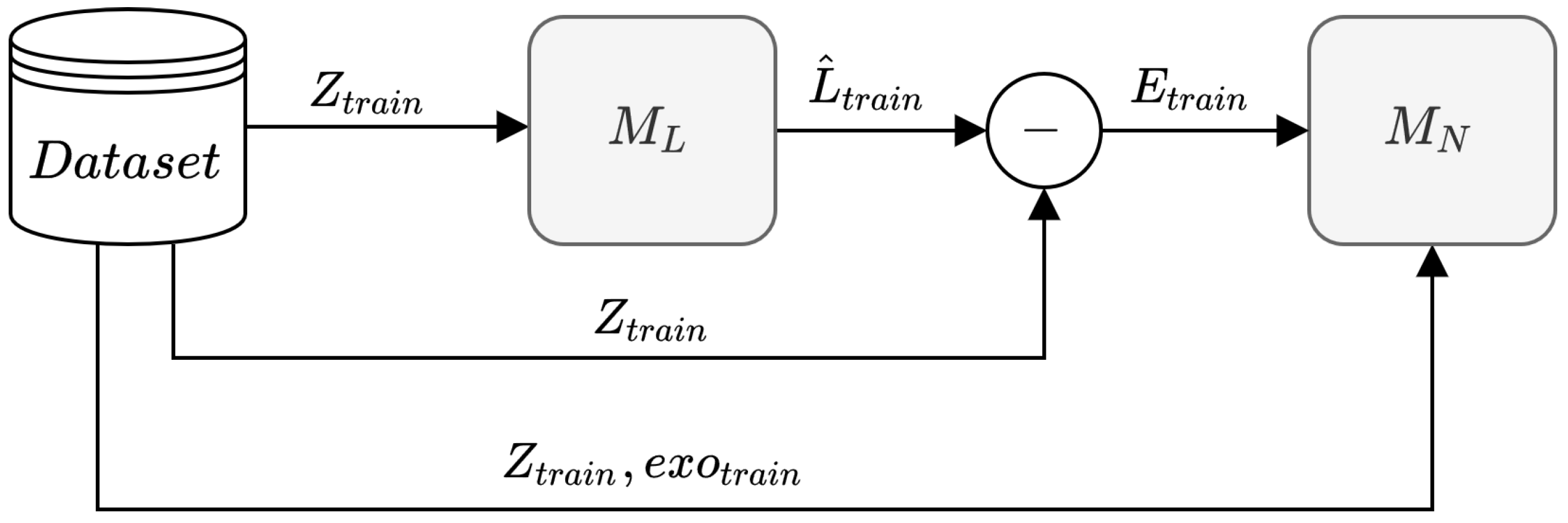
Figure 1 shows the training step of the H-Transformer. In this step, the following modules are trained:

(1)

The linear module $M_L$ is estimated using the training set $Z_{train}$. The objective is to find the SARIMA model’s parameters that generate the best linear forecast ${\widehat{L}}_{train}$ for the training set. Their outputs are the linear forecast ${\widehat{L}}_{train}$ and the trained SARIMA;

(2)

The nonlinear module $M_N$ is trained using $Z_{train}$ and $ex{o}_{train}$ as inputs to predict the residual series $E_{train}$ (Equation (4)). The output of the nonlinear module is the forecast ${\widehat{N}}_{train}$ and the trained Transformer.

In the first step of the system, the linear model $M_L$ is trained based on the n-lagged target $Z_{train}$ to predict the target one step ahead. The trained $M_L$ then outputs the linear component of the $Z_{train}$, ${\widehat{L}}_{train}$, which is used by Equation (4) to produce the residual series $E_{train}$.

$$E_{train}=Z_{train}-{\widehat{L}}_{train}.$$

(4)

The second step of the system trains a Transformer model $M_N$ using the n-lagged exogenous data $ex{o}_{train}$ and $Z_{train}$ to be able to predict the residual series $E_{train}$. The output of this step is the forecast of the nonlinear component ${\widehat{N}}_{train}$.

In the Transformer training step, a BHO [30] searches for the best parameters of the model and the best number of lags to be considered. The BHO finds the best model by minimizing the validation loss function. A summary of how the optimization works and how it was used in this work is further described in Section 4.2.

3.2. Testing Step

The testing step of the system, shown in Figure 2, uses all three modules:

1.

The trained linear module $M_L$ forecasts the next hour target $Z_{test+1}$ using the n-lagged data $Z_{test}$. It outputs the linear component ${\widehat{L}}_{test+1}$;

2.

The trained nonlinear module $M_N$ uses the n-lagged exogenous data $ex{o}_{test}$ and $Z_{test}$ to predict the nonlinear component of the target ${\widehat{N}}_{test+1}$;

3.

The combination module sums ${\widehat{L}}_{test+1}$ and ${\widehat{N}}_{test+1}$ to produce ${\widehat{Z}}_{test+1}$ (Equation (5)). The resulting forecast can then be compared with the real value $Z_{test+1}$ using loss functions such as $RMSE$ and $MAE$.

$${\widehat{Z}}_{test+1}={\widehat{L}}_{test+1}+{\widehat{N}}_{test+1}.$$

(5)

4. Experimental Setup and Results

Section 4.1, Section 4.2 and Section 4.3 present the data set description, the experimental protocol and the simulation results, respectively.

4.1. Data

This work uses five renewable energy time series (two sets of solar energy and three sets of wind speed) to assess the performance of the proposed hybrid system in the forecasting task.

The first dataset of solar energy (named $Solar1$) is composed of data obtained from a solar panel installed in the Northeast region of Brazil over a total period of one year—between the beginning of July 2018 and the end of July 2019 [31]. The dataset is composed of two files: (i) Weather data from the exact location of the solar panels, taken every minute, totaling 570,281 observations and 35 features; (ii) Data with the solar panel information, such as energy generated, taken every 15 min, totaling 38,016 observations and 18 features. These data contain null observations between 6 pm and 6 am each day and from mid-April 2019 to mid-June 2019.

The Second Dataset ($Solar2$) is composed of data obtained from a solar panel installed in India over a total period of 34 days, with observations of multiple panels every 10 min [32]. This dataset is also composed of two files, and the information of each file is as follows: (i) Weather data from the exact location of the solar panels and only three features; (ii) Data with the generated energy of multiple solar panels and one feature per solar panel.

The following Datasets ($Wind1$, $Wind2$ and $Wind3$) are composed of data obtained hourly from a wind turbine in three different regions of Northeast of the Brazil (Recife, Natal, and Fortaleza) over a total period of 1 month. Each dataset is composed of a single file containing the weather data from the exact location of the wind turbines, as well as the wind speed (target).

Preprocessing

Both datasets ($Solar1$ and $Solar2$) were resampled at 1-hour intervals, merged with their respective weather datasets, and finally cleaned of all null observations. For $Solar1$, all extra features of the solar panel data were removed, except for the power generation feature, which was used as a target for the regression of the nonlinear Models. In the case of $Solar2$, the mean of all solar panels’ generated energy was used for the target of the regression nonlinear, and all other features were removed. The wind speed datasets were already in the correct schema up to this point.

A $shift$ operation is computed to transform each observation to contain the information of its previous n timesteps, or number of lags. The choice of possible options for n was defined by the highest observations on each dataset’s autocorrelation function (ACF).

The resulting datasets (described in

Table 2. Description of the resulting datasets after the preprocessing steps.

	Solar1	Solar2	Wind1	Wind2	Wind3
Observations	4020	273	744	720	744
Features	39	3	4	4	4
Frequency	1 h	1 h	1 h	1 h	1 h
Lags	3, 6, 12, 24	3, 6, 12	1–12	1–12	1–12

) were divided into Training, Validation, and Test sets. The three sets were normalized using the min-max method described by Equation (6). $Y_i^{\prime }$ is the normalized version of the $Y_i$ data, where $min\left(Y\right)$ is the minimum occurrence and $max\left(Y\right)$ is the maximum occurrence in the Training data. The values of the transformed data are in the range [$0,1$] based on the training set. The normalization is done on each exogenous variable and target time series.

$$Y_i^{\prime }=\frac{Y_i-min\left(Y\right)}{max\left(Y\right)-min\left(Y\right)},$$

(6)

where Y is the list containing all values of an exogenous variable or time series under analysis.

4.2. Experimental Protocol

The proposed hybrid system, named H-Transformer, was compared with two literature approaches in this work: single and hybrid. The single approaches selected were the traditional statistical linear model, SARIMA, and four state-of-the-art Machine Learning models: RNN [33], LSTM [34], GRU [35], and Transformer [24]. The codes for all experimentation and tests are available on GitHub (https://github.com/nyancy/h-transformer (accessed on 23 October 2022)).

The hybrid approaches were developed based on [18], as well as the proposed H-Transformer. This paper refers to these hybrid systems as SARIMA+RNN, SARIMA+LSTM, and SARIMA+GRU.

The well-known Box and Jenkins methodology [36] was employed for selecting the hyperparameters $[p,d,q,P,D,Q,T]$ of the SARIMA model. This methodology is relevant because it guarantees that the linear patterns present in the time series be properly modeled.

The BHO method was used to design the ML models of the single and hybrid approaches. The objective of the BHO is to find the best solution while avoiding local optima. The Bayesian algorithm builds a probabilistic model that maps the hyperparameter values and the loss evaluated on validation data when optimizing hyperparameters. The optimization iteratively evaluates and updates suitable configurations by balancing exploration (avoiding local minima) and exploitation (exploiting the optimum), using this information to find the optimum of the function. Because it uses a probabilistic model, Bayesian optimization has shown better results in the literature when compared to classic hyperparameter optimization algorithms such as random search and grid search [37].

The BHO tested 50 different combinations of hyperparameters for each ML model. Each combination ran for up to 300 epochs, stopping sooner if the validation error did not improve after 15 epochs (Early Stopping). The method created 200 combinations for each dataset and model, totaling 800 runs. The search only uses training and validation sets to evaluate its performance.

The parameters and their values considered by the BHO for the RNN [33], LSTM [34], GRU [35] and Transformer [24] models were:

• units, from 4 to 256;
• learning_rate, from 0.1 to 0.001;
• batch_size, from 8 to 256;
• dropout, from 0.1 to 0.4;
• lags, depends on the dataset.

The Transformer model has a few additional parameters that are listed below. The hyperparameters considered on the original Transformer [24] constitute one of the possible configurations.

• head_size, from 64 to 256;
• head_number, from 2 to 8;
• block_number, from 2 to 8;

The loss used for optimization and comparison was the MSE (Mean Squared Error), computed by the Equation (7). The hybrid models used the SARIMA residual series as the target for the loss calculation.

$$\mathrm{MSE}=\frac{1}{n}\sum _{i=1}^n(Z_t-{\widehat{Z}}_t){}^2,$$

(7)

where $Z_t$ and ${\widehat{Z}}_t$ are the actual series and forecasting at the time t.

Two evaluation metrics were used for performance comparison: Root Mean Squared Error (RMSE) and the Mean Absolute Error (MAE). The RMSE (Equation (8)) is an evaluation metric similar to the MSE. The square root is computed to transform the error into the same scale as the data. The MSE and RMSE are more sensitive to outliers when compared to the other metrics [38].

$$\mathrm{RMSE}=\sqrt{\frac{1}{n}\sum _{i=1}^n{(Z_t-{\widehat{Z}}_t)}^2}.$$

(8)

The CV(RMSE) (Coefficient of Variation of the RMSE) (Equation (9)) calculates the ratio of the standard deviation to the mean, dividing the obtained RMSE by the mean of the time series Z $\left(\overline{Z}\right)$. It is used to indicate the amount of randomness between the data and the forecasted values. According to [39], a forecast model shall have a maximum CV(RMSE) of 25%, where lower values imply that the model outputs better forecasts.

$$\mathrm{CV}\left(\mathrm{RMSE}\right)=100\times \frac{\sqrt{\frac{1}{n}{\sum }_{i=1}^n{(Z_t-{\widehat{Z}}_t)}^2}}{\overline{Z}}.$$

(9)

The MAE, shown on Equation (10), is less sensitive to outliers when compared to the MSE and RMSE, and also provides an error value on the same scale of the data.

$$\mathrm{MAE}=\frac{1}{n}\sum _{i=1}^n|Z_t-{\widehat{Z}}_t|.$$

(10)

The percentage difference, denoted here as Gain (Equation (11)), is used to compare the performance of the H-Transformer regarding other methods used in the comparison:

$$\mathrm{Gain}=\frac{{\mathit{Metric}}_{\mathit{literature}}-{\mathit{Metric}}_{\mathit{proposed}}}{{\mathit{Metric}}_{\mathit{literature}}}·100,$$

(11)

where $Metri{c}_{proposed}$ is the RMSE or MAE obtained by the proposed H-Transformer, and $Metri{c}_{literature}$ is the obtained RMSE or MAE for the single and hybrid approach models used for comparison. Positive percentage values indicate that the proposed H-Transformer attained a higher performance metric regarding a respective literature method.

4.3. Experimental Results

Table 3. RMSE and MAE performance metrics of the H-Transformer, single and hybrid approaches for renewable time series. The best value for each time series is highlighted in bold. The error in Solar dataset predictions are in KWh, and in m/s for Wind datasets.

Model Info		Solar1		Solar2		Wind1		Wind2		Wind3
Approach	Model	RMSE	MAE	RMSE	MAE	RMSE	MAE	RMSE	MAE	RMSE	MAE
Single	SARIMA [23]	975	756	1674	1451	0.810	0.659	1.115	0.930	0.795	0.632
	RNN [33]	807	548	1568	1258	0.710	0.543	0.907	0.699	0.697	0.529
	LSTM [34]	817	570	1455	1201	0.714	0.550	0.960	0.738	0.701	0.528
	GRU [35]	793	526	1531	1176	0.680	0.511	0.849	0.656	0.681	0.503
	Transformer [24]	872	594	2438	1914	0.952	0.720	0.907	0.697	0.851	0.601
Hybrid	SARIMA + RNN	803	577	1252	939	0.637	0.482	0.847	0.653	0.673	0.539
	SARIMA + LSTM	807	580	1460	1097	0.611	0.438	0.846	0.656	0.671	0.538
	SARIMA + GRU	871	608	1300	971	0.645	0.466	0.849	0.660	0.671	0.537
	H-Transformer	766	516	1307	934	0.623	0.422	0.838	0.645	0.665	0.533

shows the results with both RMSE and MAE metrics for single and hybrid approaches on the testing set for all datasets. The error on solar datasets corresponds to power generation in KWh, while the wind datasets’ loss represents the wind speed in m/s. Since the metrics are different, Table 3 provides a comparison between models in the same dataset, not between datasets. Overall, the hybrid approaches achieved better results than respective single models. The proposed H-Transformer attained the best RMSE metrics in 3 out of 5 time series. In MAE terms, the proposal reached the best values in 4 out of 5 time series.

Table 4. CV(RMSE) performance metric of the H-Transformer, single and hybrid approaches for renewable time series. The best value for each time series is highlighted in bold.

Model Info		CV (RMSE)
Approach	Model	Solar1	Solar2	Wind1	Wind2	Wind3
Single	SARIMA [23]	27.36%	32.29%	27.61%	19.01%	20.82%
	RNN [33]	22.65%	30.24%	24.20%	15.46%	18.26%
	LSTM [34]	22.93%	28.06%	24.34%	16.37%	18.36%
	GRU [35]	22.26%	29.53%	23.18%	14.48%	17.84%
	Transformer [24]	24.47%	47.03%	32.45%	15.46%	22.29%
Hybrid	SARIMA + RNN	22.54%	24.15%	21.71%	14.44%	17.63%
	SARIMA + LSTM	22.65%	28.16%	20.83%	14.42%	17.57%
	SARIMA + GRU	24.44%	25.07%	21.99%	14.48%	17.57%
	H-Transformer	21.50%	25.21%	21.24%	14.29%	17.42%

shows the attained CV(RMSE) metric for all approaches on the testing set of all datasets using the results from Table 3. CV(RMSE) permits a comparison of the model’s performance between datasets, where lower values mean that the model outputs a better forecast. The H-Transformer achieved better performance on Wind datasets, and had a CV(RMSE) less than 25% in 4 out of 5 series.

Overall, the hybrid approaches attained better results than their single counterparts. The proposed hybrid system, the H-Transformer, outperformed all single models when analyzing the RMSE and achieved the best MAE in all datasets compared to other hybrid systems.

Figure 3 shows that in most of the time series, the H-Transformer attained a remarkable gain from other models. For instance, in all datasets, the proposed hybrid system improved the SARIMA accuracy, reaching an accuracy superior to the single Transformer model. This result corroborates the hypotheses that support the proposition of the H-Transformer. Similarly, Figure 4 shows the superior result in terms of MAE of the proposed hybrid system. For instance, the H-Transfomer attained a percentage gain greater than 30% in four out of five data sets compared to the SARIMA model. Even in the cases where other models outperformed the H-Transformer, the percentage difference is considerably low.

Figure 5 shows the forecasting for the last 100 actual values (blue line) of the five renewable energy time series used in the study. For all data sets, the comparison is performed between the forecasts of the SARIMA model(red line) and the proposed H-Transformer (green line).

It is possible to note that for all data sets, the H-Transfomer forecast is closer to the actual series than the SARIMA outputs. The difference between SARIMA and the H-Transformer is especially relevant in estimating the time series’ peaks and valleys, where reaching an accurate estimate is more challenging and relevant [11,14].

5. Conclusions

Due to the wide variation of the solar photovoltaic and the volatile nature of the wind speed, the necessity for developing accurate systems to forecast renewable energy generation has been increasing. Numerous studies have considered different methods and metrics to improve such approaches’ performance. However, issues regarding model nature, parameter selection, weather, and environmental conditions affect the performance in renewable time series forecasting.

This work proposed a hybrid system that combines the traditional linear SARIMA model with a state-of-the-art Transformer model using the residual series. The proposal, H-Transfomer, was developed for renewable energy forecast, aiming to deal with the abovementioned issues. The well-known Bayesian optimization was employed to select the best hyperparameters and the number of lags of the Transformer. In the nonlinear modeling of the residual series, exogenous data were considered in an unprecedented way to improve the accuracy of the Transformer model. The proposed hybrid system was compared with single and hybrid approaches in the literature using five renewable energy time series.

The results in terms of two well-known evaluation metrics were used to compare each model on the test set: RMSE and MAE. The hybrid system, H-Transformer, obtained the best overall result, showing that the proposal can be an interesting tool to attain accurate forecasts in the renewable energy scenario.

This research, however, is subject to limitations:

• The optimization step requires multiple executions of deep neural networks, which require high computational power. Powerful machines can execute the optimization step much faster with many more combinations, possibly outputting better results;
• There are not many open multivariate renewable energy datasets available, which limits the comparison and evaluation of the models;
• The proposed hybrid system employs a linear combination of statistical and ML models. Some works show that nonlinear combinations can be more accurate than linear ones [29] in the forecasting task;
• Selecting the perfect combination of models is challenging due to the no-free-lunch theorem [40] in search and optimization problems. Multiple variables and parameters influence the performance of each model differently, which makes the choice of models and combinations a challenging task itself.

Alternative versions of the Transformer and attention-based models have been created specifically for the time series forecasting field and produced promising results [41]. Hybrid systems improved the performance of simple Transformers for renewable energy forecast, so testing hybrid systems with those alternative Transformers is expected to output even better results.

Improvements on hybrid systems are also an attractive approach for future works. Izidio et al. [42] proposed a three-phase hybrid system for forecasting energy consumption for smart meters. Their system outperformed previously tested models. A similar hybrid system could be developed using Transformers for renewable energy forecast.

Future works may include a more comprehensive number of exogenous variables and running a feature selection on each dataset. Finally, the optimization step can be improved by increasing the number of hyperparameters and their ranges and using a more suitable fitness function [43]. As concluded by Ahmed et al. [27], evolutionary algorithms have performed well on the optimization task of renewable energy forecasting models.

References

- Taalas, P.; Guterres, A. State of the Global Climate 2020; WMO-No. 1264; WMO: Genève, Switzerland, 2021. [Google Scholar]
- Perera, F. Pollution from Fossil-Fuel Combustion is the Leading Environmental Threat to Global Pediatric Health and Equity: Solutions Exist. Int. J. Environ. Res. Public Health 2017, 15, 16. [Google Scholar] [CrossRef] [PubMed] [Green Version]
- Şen, Z. Solar energy in progress and future research trends. Prog. Energy Combust. Sci. 2004, 30, 367–416. [Google Scholar] [CrossRef]
- Elhadidy, M.; Shaahid, S. Parametric study of hybrid (wind + solar + diesel) power generating systems. Renew. Energy 2000, 21, 129–139. [Google Scholar] [CrossRef]
- Khare, V.; Nema, S.; Baredar, P. Solar–wind hybrid renewable energy system: A review. Renew. Sustain. Energy Rev. 2016, 58, 23–33. [Google Scholar] [CrossRef]
- André, T.; Brown, A.; Collier, U.; Dent, C.; Epp, B.; Gibb, D.; Kumar, C.H.; Joubert, F.; Kamara, R.; Ledanois, N.; et al. Renewables 2021 Global Status Report; REN21; c/o UN Environment Programme: Paris, France, 2021. [Google Scholar]
- Zervos, A.; Lins, C.; Muth, J. RE-Thinking 2050; European Renewable Energy Council: Brussels, Belgium, 2010. [Google Scholar]
- AlSkaif, T.; Dev, S.; Visser, L.; Hossari, M.; van Sark, W. A systematic analysis of meteorological variables for PV output power estimation. Renew. Energy 2020, 153, 12–22. [Google Scholar] [CrossRef]
- Diagne, M.; David, M.; Lauret, P.; Boland, J.; Schmutz, N. Review of solar irradiance forecasting methods and a proposition for small-scale insular grids. Renew. Sustain. Energy Rev. 2013, 27, 65–76. [Google Scholar] [CrossRef] [Green Version]
- Voyant, C.; Notton, G.; Kalogirou, S.; Nivet, M.L.; Paoli, C.; Motte, F.; Fouilloy, A. Machine learning methods for solar radiation forecasting: A review. Renew. Energy 2017, 105, 569–582. [Google Scholar] [CrossRef]
- de O. Santos, D.S.; de Mattos Neto, P.S.G.; de Oliveira, J.F.L.; Siqueira, H.V.; Barchi, T.M.; Lima, A.R.; Madeiro, F.; Dantas, D.A.P.; Converti, A.; Pereira, A.C.; et al. Solar Irradiance Forecasting Using Dynamic Ensemble Selection. Appl. Sci. 2022, 12, 3510. [Google Scholar] [CrossRef]
- Wang, Z.; Liu, W. Wind energy potential assessment based on wind speed, its direction and power data. Sci. Rep. 2021, 11, 16879. [Google Scholar] [CrossRef]
- Corizzo, R.; Ceci, M.; Fanaee-T, H.; Gama, J. Multi-aspect renewable energy forecasting. Inf. Sci. 2021, 546, 701–722. [Google Scholar] [CrossRef]
- de Mattos Neto, P.S.; de Oliveira, J.F.; de O. Santos Júnior, D.S.; Siqueira, H.V.; Marinho, M.H.; Madeiro, F. An adaptive hybrid system using deep learning for wind speed forecasting. Inf. Sci. 2021, 581, 495–514. [Google Scholar] [CrossRef]
- Das, U.K.; Tey, K.S.; Seyedmahmoudian, M.; Mekhilef, S.; Idris, M.Y.I.; Deventer, W.V.; Horan, B.; Stojcevski, A. Forecasting of photovoltaic power generation and model optimization: A review. Renew. Sustain. Energy Rev. 2018, 81, 912–928. [Google Scholar] [CrossRef]
- Raza, M.Q.; Khosravi, A. A review on artificial intelligence based load demand forecasting techniques for smart grid and buildings. Renew. Sustain. Energy Rev. 2015, 50, 1352–1372. [Google Scholar] [CrossRef]
- de Marcos, R.A.; Bello, A.; Reneses, J. Electricity price forecasting in the short term hybridising fundamental and econometric modelling. Electr. Power Syst. Res. 2019, 167, 240–251. [Google Scholar] [CrossRef]
- Zhang, G. Time series forecasting using a hybrid ARIMA and neural network model. Neurocomputing 2003, 50, 159–175. [Google Scholar] [CrossRef]
- Giorgi, M.G.D.; Congedo, P.M.; Malvoni, M. Photovoltaic power forecasting using statistical methods: Impact of weather data. IET Sci. Meas. Technol. 2014, 8, 90–97. [Google Scholar] [CrossRef]
- Pedro, H.T.; Coimbra, C.F. Assessment of forecasting techniques for solar power production with no exogenous inputs. Sol. Energy 2012, 86, 2017–2028. [Google Scholar] [CrossRef]
- Mandal, P.; Madhira, S.T.S.; haque, A.U.; Meng, J.; Pineda, R.L. Forecasting Power Output of Solar Photovoltaic System Using Wavelet Transform and Artificial Intelligence Techniques. Procedia Comput. Sci. 2012, 12, 332–337. [Google Scholar] [CrossRef] [Green Version]
- Yang, X.; Jiang, F.; Liu, H. Short-Term Solar Radiation Prediction based on SVM with Similar Data. In Proceedings of the 2nd IET Renewable Power Generation Conference (RPG 2013), Beijing, China, 9–11 September 2013; Institution of Engineering and Technology: London, UK, 2013. [Google Scholar] [CrossRef]
- de Oliveira, J.F.L.; Silva, E.G.; de Mattos Neto, P.S.G. A Hybrid System Based on Dynamic Selection for Time Series Forecasting. IEEE Trans. Neural Netw. Learn. Syst. 2022, 33, 3251–3263. [Google Scholar] [CrossRef]
- Vaswani, A.; Shazeer, N.; Parmar, N.; Uszkoreit, J.; Jones, L.; Gomez, A.N.; Kaiser, L.; Polosukhin, I. Attention Is All You Need. arXiv 2017, arXiv:cs.CL/1706.03762. [Google Scholar]
- xiang Zhao, H.; Magoulès, F. A review on the prediction of building energy consumption. Renew. Sustain. Energy Rev. 2012, 16, 3586–3592. [Google Scholar] [CrossRef]
- Wang, Z.; Srinivasan, R.S. A review of artificial intelligence based building energy use prediction: Contrasting the capabilities of single and ensemble prediction models. Renew. Sustain. Energy Rev. 2017, 75, 796–808. [Google Scholar] [CrossRef]
- Ahmed, R.; Sreeram, V.; Mishra, Y.; Arif, M. A review and evaluation of the state-of-the-art in PV solar power forecasting: Techniques and optimization. Renew. Sustain. Energy Rev. 2020, 124, 109792. [Google Scholar] [CrossRef]
- Hyndman, R.J.; Athanasopoulos, G. Forecasting: Principles and Practice; OTexts: Melbourne, Australia, 2018. [Google Scholar]
- Taskaya-Temizel, T.; Casey, M.C. A comparative study of autoregressive neural network hybrids. Neural Netw. 2005, 18, 781–789. [Google Scholar] [CrossRef] [PubMed] [Green Version]
- Snoek, J.; Larochelle, H.; Adams, R.P. Practical Bayesian Optimization of Machine Learning Algorithms. arXiv 2012, arXiv:1206.2944. [Google Scholar]
- Ribeiro, K.; Santos, R.; Saraiva, E.; Rajagopal, R. A Statistical Methodology to Estimate Soiling Losses on Photovoltaic Solar Plants. J. Sol. Energy Eng. 2021, 143, 064501. [Google Scholar] [CrossRef]
- Kannal, A. Solar Power Generation Data. 2020. Available online: https://www.kaggle.com/datasets/anikannal/solar-power-generation-data (accessed on 23 October 2022).
- Abadi, M.; Agarwal, A.; Barham, P.; Brevdo, E.; Chen, Z.; Citro, C.; Corrado, G.S.; Davis, A.; Dean, J.; Devin, M.; et al. TensorFlow: Large-Scale Machine Learning on Heterogeneous Systems. 2015. Software. Available online: tensorflow.org (accessed on 23 October 2022).
- Hochreiter, S.; Schmidhuber, J. Long short-term memory. Neural Comput. 1997, 9, 1735–1780. [Google Scholar] [CrossRef]
- Cho, K.; van Merrienboer, B.; Gulcehre, C.; Bahdanau, D.; Bougares, F.; Schwenk, H.; Bengio, Y. Learning Phrase Representations using RNN Encoder–Decoder for Statistical Machine Translation. In Proceedings of the 2014 Conference on Empirical Methods in Natural Language Processing (EMNLP), Doha, Qatar, 25–29 October 2014; Association for Computational Linguistics: Stroudsburg, PA, USA, 2014. [Google Scholar] [CrossRef]
- Box, G. Time Series Analysis: Forecasting and Control; Jons Wiley & Sons: Hoboken, NJ, USA, 2008. [Google Scholar]
- Shahriari, B.; Swersky, K.; Wang, Z.; Adams, R.P.; de Freitas, N. Taking the Human Out of the Loop: A Review of Bayesian Optimization. Proc. IEEE 2016, 104, 148–175. [Google Scholar] [CrossRef] [Green Version]
- Hyndman, R.J.; Koehler, A.B. Another look at measures of forecast accuracy. Int. J. Forecast. 2006, 22, 679–688. [Google Scholar] [CrossRef] [Green Version]
- American Society of Heating, Refrigerating; Air-Conditioning Engineers. Ashrae Guideline 14-2014: Measurement of Energy, Demand and Water Savings; American Society of Heating, Refrigerating, and Air-Conditioning Engineers: Peachtree Corners, GA, USA, 2014. [Google Scholar]
- Wolpert, D.; Macready, W. No free lunch theorems for optimization. IEEE Trans. Evol. Comput. 1997, 1, 67–82. [Google Scholar] [CrossRef]
- Simeunović, J.; Schubnel, B.; Alet, P.J.; Carrillo, R.E. Spatio-temporal graph neural networks for multi-site PV power forecasting. arXiv 2021, arXiv:cs.LG/2107.13875. [Google Scholar] [CrossRef]
- Izidio, D.M.F.; de Mattos Neto, P.S.G.; Barbosa, L.; de Oliveira, J.F.L.; da Nóbrega Marinho, M.H.; Rissi, G.F. Evolutionary Hybrid System for Energy Consumption Forecasting for Smart Meters. Energies 2021, 14, 1794. [Google Scholar] [CrossRef]
- Rodrigues, L.J.A.; de Mattos Neto, P.S.G.; Ferreira, T.A.E. A prime step in the time series forecasting with hybrid methods: The fitness function choice. In Proceedings of the 2009 International Joint Conference on Neural Networks, Atlanta, GA, USA, 14–19 June 2009; pp. 2703–2710. [Google Scholar] [CrossRef]
Figure 1.
H-Transformer training step.
Figure 2.
H-Transformer testing step.
Figure 3.
The percentage difference (Equation (11)) between H-Transformer and literature methods in terms of RMSE.
Figure 4.
The percentage difference (Equation (11)) between H-Transformer and literature methods in terms of MAE.
Figure 5.
Comparison between the actual renewable energy time series (100 last points—blue line) and the forecasts of SARIMA (red line) and the H-Transformer (green line). Solar dataset predictions are measured in KWh, and Wind dataset predictions are measured in m/s.