
Contact Analysis and Friction Prediction of Non-Gaussian Random Surfaces

1
School of Mechanical Engineering and Automation, Northeastern University, Shenyang 110819, China
2
School of Science, Northeastern University, Shenyang 110819, China
*
Author to whom correspondence should be addressed.
Appl. Sci. 2022, 12(21), 11237; https://doi.org/10.3390/app122111237
Submission received: 1 October 2022
/
Revised: 20 October 2022
/
Accepted: 31 October 2022
/
Published: 5 November 2022
(This article belongs to the Special Issue Advances in Nonlinear Dynamics and Mechanical Vibrations)
Abstract
:Engineering surfaces exhibit asymmetrical height distributions due to certain types of surface finishing and running-in process. This non-Gaussian surface reflects different contact performances and tribological properties. In this paper, the influence of non-Gaussian surface parameters on contact performance and friction is investigated. First, the computer program for generating rough surfaces with given parameters is developed; then, contact analysis for rough surfaces are conducted through a deterministic contact model; finally, friction coefficient can be derived from friction model using the results of the contact model. The simulation analyses indicate that the skewness and amplitude of non-Gaussian surface have significant effects on contact performance and friction. The contact characteristic parameters and friction coefficient become slightly changed when kurtosis becomes relatively large.
1. Introduction
The friction between contact surfaces is demonstrated as an important source of nonlinear vibrations in many mechanical and structural systems. Moreover, the vibration could help reflect the health status of the machine [1,2], which has been studied widely [3,4,5,6,7,8]. Therefore, it is vital to investigate the friction characteristics. The friction behavior at the macroscopic length scale is highly correlated with the microscopic topography of the contacting surfaces, which determines the contact and lubrication status of machinery elements [9]. Over the past few decades, many analytical and numerical contact models for rough surfaces which assumed a Gaussian distribution of surface heights have been developed. In fact, some certain types of surface finishing and the running-in processes of machine operation often results in the asymmetric distribution of roughness heights. Compared with Gaussian surface, non-Gaussian surface reflects different tribological properties due to the impacts of skewness and kurtosis. Therefore, a thorough awareness of contact performance and tribological property of non-Gaussian contact surfaces is of great concern for enhancing effectiveness and reducing friction losses.
The solution of contact models demands the input of an either two- or three-dimensional rough profile which can be acquired either from digital output of the profilometer or from numerical simulations. Compared with the measured rough surfaces, the numerical method has many advantages in high efficiency and low cost. Additionally, it can efficiently generate arbitrarily and sufficiently large samples of profiles [10,11,12]. The engineering surface can be mathematically approximated as a description of stochastic process. In addition, most of the statistical parameters of an engineering surface can be sufficiently described with the use of the height distribution function and the autocorrelation function (ACF) [13]. Thus, it is convenient to generate surfaces with predetermined ACFs and the height distribution functions to take the place of engineering surfaces [14]. Patir [15] used linear transformation of a random matrix and moving average (MA) model to generate Gaussian and non-Gaussian rough surfaces with specified ACFs. However, Patir’s method required solving a nonlinear system of equations to obtain an autocorrelation coefficient matrix, which is both storage space and time limiting. In order to deal with those disadvantages, Bakolas [10] transformed the nonlinear system of equations into a nonlinear optimization problem and used the nonlinear conjugate gradient method (NCGM) with secant line search to solve. In addition, based on a 2D digital filter and Fast Fourier Transform (FFT), a fast and convenient procedure firstly proposed by Hu and Tonder [16] also were applied to generate rough surfaces. Wu [17,18] found that there were large errors between the intended ACF and the actual ACF for surfaces generated by FFT methods, especially when autocorrelation lengths became long. In addition, he modified the FFT method to obtain Gaussian and non-Gaussian surface with large wavelengths. The FFT algorithm also was adopted to the computation process of the optimization problem first presented by Patir, and many advances were made in terms of computing power and efficiency [12,19,20]. These have made Patir’s method to generate surfaces with large autocorrelation accurately. Hence, the improved Patir’s method is adopted to generate non-Gaussian surfaces in this paper.
During the past decades, many analytical and numerical models have been proposed for contact simulation of rough surfaces. In general, existing contact models can be divided into two broad categories: stochastic methods and deterministic methods. The original stochastic model was constructed by Greenwood and Williamson [21]. Various extensions of the GW contact model have been developed to incorporate the interaction between asperities and the effects of adhesion and plastic deformation [22,23,24,25,26]. However, such method cannot give the pressure distribution. The deterministic method can provide pressure distribution, deformation, etc. However, the deterministic method may have a convergence problem and calculation efficiency for large scale calculations. In order to cope with those problems, the discrete convolution-Fast Fourier transform (DC-FFT) [27] method is used extensively to speed up the related calculations by reducing the computational complexity. Polonsky and Keer [28] proposed an alternative numerical method based on the conjugate gradient method (CGM) to address the rough contact problem. Those improvements make this method converge for arbitrary rough surfaces. From this, it has been widely applied to investigate the contact properties of the non-Gaussian rough surface [29,30,31,32].
Friction is a combined phenomenon that originates from the interaction of deformation of surface irregularities and adhesive forces between the two surfaces. Thus, the surface roughness fundamentally influences friction behavior. Many researchers [33,34,35,36,37] have investigated the impact of surface topography on the friction coefficient and found that the static friction coefficient was highly sensitive to surface roughness. However, most of them used the stochastic method which were based on simplifying assumptions about the distribution of contact pressure in and around the contact region. In addition, only the effect of adhesion force on friction was considered, while the ploughing component was ignored. It is now generally agreed that friction is attributed to the interactions of the ploughing effect and adhesion force of contact asperities. Zhang [38] proposed a numerical approach based on molecular and mechanical theory to investigate the sliding friction behaviors. However, the research focused on Gaussian surface. Extensive experimental work [39,40] has been performed to investigate the correlation between roughness parameters and friction, and it was discovered that the skewness and kurtosis of non-Gaussian surface tend to have an influence on the coefficient of friction. Herein, a novel friction prediction model considering the effects of adhesion and ploughing components simultaneously is proposed and is used to derive the macroscale friction coefficient from microscale asperity interactions.
Many significant works have been completed for contact problem and friction of non-Gaussian surface; however, a systematic study to investigate the impact of non-Gaussian surface properties on contact performance and friction is still desirable. In this paper, the non-Gaussian rough surfaces with specified amplitude parameters and ACF are generated based on linear transformation and the MA model. The contact analysis is conducted by a deterministic contact model to obtain deformation of asperities contact pressure and real contact area. Then, the friction coefficient of each single asperity can be derived from the friction model using the results of the contact model. Finally, the overall friction coefficient is calculated from the sum of the friction of all asperities.
2. Methodology
2.1. Methodology for Non-Gaussian Rough Surface Generation
In this section, a generation program based on linear transformation and MA model is developed to produce a non-Gaussian rough surface with expected height distribution and ACF. The ACF describes the general dependence of the values of the dates at one location to their values at another location. It is crucial for generating random rough surfaces because it supplies fundamental information about the wavelength and the amplitude properties of rough surfaces. In this paper, the typically exponential type of ACF is adopted. It can be given below:
where is standard deviation of the rough surface heights, and represents the autocorrelation lengths in the x direction. is the length at which ACF decays to 0.1 of its value in origin position.
Based on Patir’s method, the random surface can be generated by linear transformation between a random sequence and a transform matrix :
The random sequence is independent and has unit variance; hence, it satisfies the following formula:
According to the property of ACF, the relationship between transform coefficients and the values of ACF can be expressed as:
Therefore, the transform coefficients can be obtained by solving nonlinear equations represented by Equation (4). Initially, Patir adopted the Newton method to determine the transform. The initial approximation of is given as:
where , .
However, with the increased number of nonlinear equations, the convergence problem becomes more severe. Moreover, it requires more computer memory space to store the Jacobian matrix. To cope with the efficiency and the storage space, Bakolas [10] transformed the nonlinear system of equations to a nonlinear optimization problem and use NCGM to solve. Recently, Liao et al. [12] proposed an improved numerical modeling by transforming the problem described by Patir to the nonlinear squares problem. The transformation can be rewritten as:
where is the objective function, and its gradient can be given by:
The analytical formula of gradient function with respect to each of the transform coefficient is shown as follows:
Through this transformation, the NCGM was implemented into Equation (8) for solving the nonlinear system of equations depicted in Equation (4). In addition, the FFT method can be applied to the computation of Equation (4) to improve the calculation efficiency dramatically.
Once the transform coefficients are obtained, the Gaussian surface can be generated through convolution between the transform matrix and the Gaussian random sequence . Different from Gaussian surfaces, the generation of non-Gaussian surfaces requires that the random sequence is subject to a non-Gaussian distribution. The prescribed non-Gaussian sequence with desired skewness and kurtosis can be generated by feeding the Gaussian random sequence into the Johnson translation system. The translation system involves three main types of curves, , ,
- The unbound system ;
- The logarithm normal system where ;
- The bounded system where .
where represents Gaussian random series, and represents the non-Gaussian random series with desired skewness and kurtosis. The parameters and are used to identify the statistical distribution of the non-Gaussian sequence. Those four parameters can be calculated through the expected mean value, standard deviation, skewness, and kurtosis.
In addition, the linear transformation as a pure MA process would change the kurtosis and skewness of the input random series slightly. The relations for input skewness and kurtosis and output skewness and kurtosis can be given as:
Therefore, the skewness and kurtosis which are fed into the Johnson translator system should be modified according to Equations (9) and (10). In summary, the following general procedure should be carried out for generating the non-Gaussian surfaces:
- Determine the transform coefficients through solving the nonlinear equations described by Equation (4);
- Modify the input kurtosis and skewness using Equations (9) and (10);
- Generate the random sequence, and then substitute the sequence and the modified skewness and kurtosis into the Johnson translation system for obtaining the prescribed non-Gaussian sequence;
- Generate the non-Gaussian surface with specified height distribution and ACF through linear transformation between the transform coefficients and the non-Gaussian sequence.
The generation of non-Gaussian surface is presented schematically in Figure 1.
2.2. Friction Model
Friction is a mechanical resistance for transmitting tangential forces when one surface moves over another. At the micrometer level, the engaging surfaces always exhibit protrusions and depressions, and mechanical contact occurs primarily on the asperity summits. At present, the topography of the contact surfaces is considered to influence the friction behavior at the macroscopic scale. In this section, a friction coefficient prediction model is established to investigate the effect of micro-rough interactions on the friction behavior. When rough surfaces come into contact, the applied load is shared by protrusions. Therefore, the overall friction coefficient determined by the ratio of the sum of all asperity frictions to the normal force can be expressed as
where W indicates the applied normal load; and , , and represent the friction coefficient, friction force, and normal load of individual asperities, respectively.
The macroscale friction behavior of the engaging surfaces can be characterized by investigating the friction mechanics of single asperities. To address the behaviors of a single asperity, they were modeled as perfect protuberances of conical shapes for convenience. During the contact of two asperities at the microscale, adhesion and deformation (plowing) at asperity summits collectively contribute to friction. Figure 2 depicts a schematic of the single-asperity friction model.
In the case of elastic contact, the contribution of asperity elastic deformation to friction can be negligible. Therefore, the overall friction force is equivalent to the interfacial adhesion force, which can be expressed as
where denotes the interfacial contact width, and indicates the interfacial shear strength, which varies with the contact pressure. Mishra et al. [41] conducted boundary-layer shearing experiments under different lubricant conditions. They determined the shear strength at different nominal pressures, which can be calculated using , where and are model parameters, and denotes the maximum contact pressure in the contact width . Furthermore, and were used for the unlubricated condition. Consequently, the friction coefficient of the elastic contact can be expressed as
Plastic deformation occurs when the contact pressure exceeds ; in other words, , where denotes the yield stress that can be estimated as . Herein, denotes the hardness of the material. Owing to the appearance of plastic deformation, part of the deformed asperity was assumed to penetrate the substrate. Under this condition, the plowing effect of asperity combined with interfacial adhesion contributed to the friction force during sliding. The friction coefficient formula proposed by Kragelsky et al. [42] is presented in Equation (14). This was obtained from the conical model to estimate the contributions of both adhesion and plowing mechanisms to the total friction force:
where denotes the attack angle, which is determined by the penetration depth and contact width . and indicate the interfacial and metal shear strengths, respectively. Therefore, the ratio can assume values between zero and unity depending on the interfacial conditions. In this study, an intermediate value of 0.6 was adopted in the elastic–plastic interaction.
Complete plastic deformation occurred when the contact pressure approached material hardness. The contribution of interfacial adhesion to friction was negligible. Therefore, the first part of Equation (14) indicates that only the plowing mechanism remains, and Equation (14) can be rewritten as
2.3. A Deterministic Contact Model of Rough Surfaces
The typical contact, such as gears, roller bearings, and cams, can be treated as the contact of two rollers. Furthermore, it can be simplified as the contact of elastic cylinder on a rigid surface. Consequently, the gap between the two surfaces can be expressed as
where denotes the initial geometric gap, indicates the x-coordinate of the contact area, represents the equivalent radius of curvature, and denotes the surface topography. Additionally, represents the combined surface deformations and can be determined using Green’s function approach, as follows:
where and indicate the starting and ending points of the calculation domain of the contact area, respectively, and denotes the influence kernel function determined as
where denotes the equivalent Young’s modulus. To achieve rapid computation of the deformations, the discrete convolute fast Fourier transformation algorithm, first proposed by Liu and Wang [26], was implemented within the computational domain.
The resulting pressure distribution must be consistent with the load balancing condition:
where denotes the force per unit width, and indicates the contact pressure. The pressure gap complementary boundary constraints can be written as follows:
The pressure distribution and deformations can be determined by applying the NCGM [27,28] to the load balance equation with two complementary boundary conditions. In the existing numerical analyses of rough contacts, a limiting pressure, commonly set to the material hardness, is applied to compensate for the potential yielding of plastic at the maximum stress of asperity microcontacts. This approximation yields more accurate results than a purely elastic contact model for surfaces with sharp asperities [28].
3. Validation of the Current Method
The generated non-Gaussian surface with , and is shown in Figure 3a. This is to be expected as the negatively skewed surface shows blunt asperity tip and more shape valleys. The comparison of ACF between the generated surface and the expected surface is displayed in Figure 3b. It can be observed that the ACF of the generated surface matches excellently with the prescribed values. The results demonstrate the validity of the mothed for generating a prescribed non-Gaussian surface.
A commercial twin-disc test implemented by Zhang et al. [38] is used to validate the prediction model of friction coefficient proposed in Section 2.2. The validation experiment was performed under different surface conditions and applied loads. The two surface roughness conditions are Rq surface roughness of 0.28 and 0.47 , which are shown in Figure 4. Friction coefficients were acquired at two linear loads of and for each set of surface roughness conditions. The detailed test parameters are summarized in Table 1. The contact pressure and gap under four sets of operating conditions are illustrated in Figure 5. As can be seen in Figure 6, the numerical results of current method demonstrate good agreement with the results of the experiment.
4. Results and Discussion
In order to survey the impact of non-Gaussian surface parameters on contact properties and friction, rough surfaces with different standard deviation , skewness , and kurtosis are generated based on the program developed in Section 2.1. The detailed parameters are summarized in Table 2. Then, the contact analysis is implemented to predict the friction coefficient based on the model introduced in Section 2.2. The contact analysis consists of a smooth sphere of radius 40 mm against a rough elastic–plastic plane, whose Young’s modulus is , Poisson’s ratio is , and material hardness H is set as . A set of applied loads from to are adopted to survey the effect of the load.
4.1. Effect of Roughness Amplitude and Skewness
As indicated in Figure 7a,b, the rough surface with negative skewness presents blunt peaks and more sharp valleys, as opposed to a surface with a positive skewness. Those result in different contact performances and friction behavior. As demonstrated in Figure 8, it is evident that, when the surface with positive skewness comes into contact, larger contact pressures are observed at most contact points compared to the negatively skewed surface. The reason for this is that the surface with the positive skewness has less summits to sustain the applied load, leading to higher local pressure. In turn, the negatively skewed surface with more flat protrusions results in a larger contact area, leading to lower contact pressure.
Based on the friction theory introduced in Section 2.2, a friction coefficient is influenced by contact pressure, contact deformation, and contact area. Under elastic contact, the interfacial adhesion dominates the overall friction. When the contact pressure exceeds the material yield, the plowing effect of asperity combined with interfacial adhesion collectively contribute to the friction during sliding. In this paper, the average contact pressure, plastic ratio, and contact area ratio are used as the indications to represent the trend of contact pressure, contact deformation, and contact area. The average contact pressure represents the average of the pressures of all contact points. The contact area ratio is evaluated as the real contact area divided by the Hertzian contact area. Similarly, the plastic ratio is determined as the ratio of the number of contact points where contact pressure exceeds the material yield to the number of contact points. To account for the effect of the amplitude parameter, contact analyses were performed on a series of rough surfaces with identical skewness and different amplitudes. The numerical calculations are displayed in Figure 9 and Figure 10. Figure 9 shows that the trend of friction coefficient is similar for negatively skewed surfaces and positively skewed surfaces. Initially, a friction coefficient has a slightly decreasing trend. This is because the friction coefficient is dominated by interfacial adhesion for relatively smooth surfaces. As the roughness amplitude increases, the actual contact area presents a significant reduction. A further increase in surface roughness amplitude leads to an increase in local contact pressure. As depicted in Figure 10, the average contact pressure increases with increasing roughness amplitude. Consequently, the increase in local pressure causes an increase in the plastic ratio, resulting in a significant increase in the plowing effect. Finally, the plowing mechanism becomes important role in determining friction of the rough surface. The distinction between negatively skewed surfaces and positively skewed surfaces is that the changes of average contact pressure, contact area ratio, and the plastic ratio of surfaces with positive skewness are more dramatic.
4.2. Effect of Kurtosis
Rough surfaces with different kurtosis and the same skewness and standard deviation showed obvious distinctions in peak-to-mean and asperity density. Here, peak-to-mean is the distance between the highest peak and the mean line. As shown in Figure 11, rough surface tends to increase in peak-to-mean distance and decrease in peak density as kurtosis increases. Therefore, as expected, these result in an increase in local contact pressure because of the reduction in the contact area. The contact area ratio, average contact pressure, and plastic ratio as the functions of kurtosis under uniform skewness and linear load are presented in Figure 12. It is observed that, due to rough surfaces with high kurtosis having higher and sharper peaks, the number of contact asperities start to decrease, contributing to an increase in contact pressure and a decrease in contact area. The increase in contact pressure may induce a large degree of plastic deformation. However, for high kurtosis values (), the impact of kurtosis becomes limited. The variations of contact area and pressure become slight. The similar trends are also observed by [28,34,43]. In Figure 12, the observation about friction coefficient is that the influence of kurtosis on friction coefficient is very slight, especially for . This trend is consistent with Liu’s experimental study [43].
4.3. Effects of Applied Load
In this section, a set of applied loads from to are conducted to contact analysis for surveying the effects of applied load. A non-Gaussian surface of and , as shown in Figure 13, is adopted. As presented in Figure 14, contact area increases with increasing applied load. However, contact pressure displays different trends. For a relatively small load, contact pressure increases with the increase of contact area. A further increase in applied load enhances the Hertzian width, resulting in more asperities to sustain the applied load. This causes the reduction of contact pressure and average contact pressure, as indicated in Figure 15. Thus, the plastic ratio presents an obvious increasing trend for a relatively small load, and then gets saturated gradually with the increase of applied load. A friction coefficient shows a similar trend with the plastic ratio. The increasing trend of a friction coefficient in a relatively small load results from the increase in contact area and pressure. Finally, the friction coefficient becomes constant with an increase in applied load.
5. Conclusions
Throughout this paper, a numerical method is prepared to produce non-Gaussian surface with the specified amplitude parameters and ACF. A deterministic contact model is used to investigate the contact behaviors of non-Gaussian surfaces with different skewness, kurtosis, roughness amplitude, and applied load. A friction coefficient can be derived by a proposed friction model. The main conclusions are drawn as follows:
- 1.
- Rough surfaces with positive skewness, because of more sharp peaks and less valleys, present larger contact pressure as well as a smaller contact area than the negatively skewed surfaces. With the increasing of roughness amplitude, the contact pressure increases, while the contact area decreases, both for the surface with positive skewness and negative skewness. In addition, the trends of friction coefficients with increasing roughness amplitude are similar for negatively skewed surfaces and positively skewed surfaces.
- 2.
- As the kurtosis increases, the contact area decreases while the contact pressure increases. Nevertheless, when the kurtosis becomes comparatively large, the variations of contact area and pressure become slight. The influence of kurtosis on friction coefficient is very slight, especially for .
- 3.
- The contact area increases as applied load increases. However, contact pressure first presents a clear increasing trend and then gradually declines because of more asperities coming into contact. Similar to the trend of contact pressure, friction coefficient first increases due to the increase in contact area and pressure, finally becoming constant.
Author Contributions
Conceptualization, J.R. and H.Y.; methodology, H.Y.; software, J.R.; validation, J.R. and H.Y.; formal analysis, J.R.; investigation, J.R.; resources, H.Y.; data curation, H.Y.; writing—original draft preparation, J.R.; writing—review and editing, J.R.; supervision, H.Y.; project administration, H.Y.; All authors have read and agreed to the published version of the manuscript.
Funding
This research was funded by National Science Foundation of China, grant number No. 51775093.
Institutional Review Board Statement
Not applicable.
Informed Consent Statement
Not applicable.
Data Availability Statement
Not applicable.
Conflicts of Interest
The authors declare no conflict of interest.
References
- Feng, K.; Ji, J.C.; Li, Y.; Ni, Q.; Wu, H.; Zheng, J. A novel cyclic-correntropy based indicator for gear wear monitoring. Tribol. Int. 2022, 171, 107528. [Google Scholar] [CrossRef]
- Feng, K.; Ji, J.; Ni, Q. A novel adaptive bandwidth selection method for Vold–Kalman filtering and its application in wind turbine planetary gearbox diagnostics. Struct. Health Monit. 2022, 2022, 14759217221099966. [Google Scholar] [CrossRef]
- Zhao, T.Y.; Jiang, L.P.; Pan, H.G.; Yang, J.; Kitipornchai, S. Coupled free vibration of a functionally graded pre-twisted blade-shaft system reinforced with graphene nanoplatelets. Compos. Struct. 2021, 262, 113362. [Google Scholar] [CrossRef]
- Zhao, T.Y.; Cui, Y.S.; Pan, H.G.; Yuan, H.Q.; Yang, J. Free vibration analysis of a functionally graded graphene nanoplatelet reinforced disk-shaft assembly with whirl motion. Int. J. Mech. Sci. 2021, 197, 106335. [Google Scholar] [CrossRef]
- Zhao, T.Y.; Yan, K.; Li, H.W.; Wang, X. Study on theoretical modeling and vibration performance of an assembled cylindrical shell-plate structure with whirl motion. Appl. Math. Model. 2022, 110, 618–632. [Google Scholar] [CrossRef]
- Zhao, T.; Li, K.; Ma, H. Study on dynamic characteristics of a rotating cylindrical shell with uncertain parameters. Anal. Math. Phys. 2022, 12, 97. [Google Scholar] [CrossRef]
- Zhao, T.Y.; Ma, Y.; Zhang, H.Y.; Pan, H.G.; Cai, Y. Free vibration analysis of a rotating graphene nanoplatelet reinforced pre-twist blade-disk assembly with a setting angle. Appl. Math. Model. 2021, 93, 578–596. [Google Scholar] [CrossRef]
- Zhao, T.Y.; Wang, Y.X.; Pan, H.G.; Yuan, H.Q.; Yi, C. Nonlinear forced vibration analysis of spinning shaft-disk assemblies under sliding bearing supports. Math Models Methods Appl. Sci. 2021, 44, 12283–12301. [Google Scholar] [CrossRef]
- Feng, K.; Ji, J.C.; Ni, Q.; Beer, M. A review of vibration-based gear wear monitoring and prediction techniques. Mech. Syst. Signal Process. 2023, 182, 109605. [Google Scholar] [CrossRef]
- Bakolas, V. Numerical generation of arbitrarily oriented non-Gaussian three-dimensional rough surfaces. Wear 2003, 254, 546–554. [Google Scholar] [CrossRef]
- Reizer, R. Simulation of 3D Gaussian surface topography. Wear 2011, 271, 539–543. [Google Scholar] [CrossRef]
- Liao, D.; Shao, W.; Tang, J.; Li, J. An improved rough surface modeling method based on linear transformation technique. Tribol. Int. 2018, 119, 786–794. [Google Scholar] [CrossRef]
- Whitehouse, D.J. Handbook of Surface Metrology; Institute of Physics: Bristol, UK, 1994. [Google Scholar]
- Manesh, K.K.; Ramamoorthy, B.; Singaperumal, M. Numerical generation of anisotropic 3D non-Gaussian engineering surfaces with specified 3D surface roughness parameters. Wear 2010, 268, 1371–1379. [Google Scholar] [CrossRef]
- Patir, N. A numerical procedure for random generation of rough surfaces. Wear 1978, 47, 263–277. [Google Scholar] [CrossRef]
- Hu, Y.Z.; Tonder, K. Simulation of 3-D random rough surface by 2-D digital filter and fourier analysis. Int. J. Mach. Tools Manuf. 1992, 32, 83–90. [Google Scholar] [CrossRef]
- Wu, J.J. Simulation of rough surfaces with FFT. Tribol. Int. 2000, 33, 47–58. [Google Scholar] [CrossRef]
- Wu, J.-J. Simulation of non-Gaussian surfaces with FFT. Tribol. Int. 2004, 37, 339–346. [Google Scholar] [CrossRef]
- Francisco, A.; Brunetière, N. A hybrid method for fast and efficient rough surface generation. Proc. Inst. Mech. Eng. Part J. J. Eng. Tribol. 2016, 230, 747–768. [Google Scholar] [CrossRef]
- Watson, M.; Lewis, R.; Slatter, T. Improvements to the linear transform technique for generating randomly rough surfaces with symmetrical autocorrelation functions. Tribol. Int. 2020, 151, 106487. [Google Scholar] [CrossRef]
- Greenwood, J.A.; Williamson, J.B.P. Contact of nominally flat surfaces. Proc. R. Soc. Lond. Ser. A 1966, 295, 300–319. [Google Scholar]
- Zhao, Y.; Maietta, D.M.; Chang, L. An asperity microcontact model incorporating the transition from elastic deformation to fully plastic flow. ASME J. Tribol. 2000, 122, 86–93. [Google Scholar] [CrossRef]
- Greenwood, J.A. A simplified elliptical model of rough surface contact. Wear 2006, 261, 191–200. [Google Scholar] [CrossRef]
- Ciavarella, M.; Greenwood, J.A.; Paggi, M. Inclusion of “interaction” in the Greenwood and Williamson contact theory. Wear 2008, 265, 729–734. [Google Scholar] [CrossRef]
- Paggi, M.; Ciavarella, M. The coefficient of proportionality k between real contact area and load, with new asperity models. Wear 2010, 268, 1020–1029. [Google Scholar] [CrossRef]
- Greenwood, J.A.; Putignano, C.; Ciavarella, M.A. Greenwood & Williamson theory for line contact. Wear 2011, 270, 332–334. [Google Scholar]
- Liu, S.B.; Wang, Q.; Liu, G. A versatile method of discrete convolution and FFT (DC-FFT) for contact analyses. Wear 2000, 243, 101–111. [Google Scholar] [CrossRef]
- Polonsky, I.A.; Keer, L.M. A numerical method for solving rough contact problems based on the multi-level multi-summation and conjugate gradient techniques. Wear 1999, 231, 206–219. [Google Scholar] [CrossRef]
- Kim, T.W.; Bhushan, B.; Cho, Y.J. The contact behavior of elastic/plastic nonGaussian rough surfaces. Tribol. Lett. 2006, 22, 1–13. [Google Scholar] [CrossRef]
- Chen, W.W.; Wang, Q.J.; Liu, Y.; Chen, W.; Cao, J.; Xia, C.; Lederich, R. Analysis and convenient formulas for elastoplastic contacts of nominally flat surfaces: Average gap, contact area ratio, and plastically deformed volume. Tribol. Lett. 2007, 28, 27–38. [Google Scholar] [CrossRef]
- Wang, Z.J.; Wang, W.Z.; Hu, Y.Z.; Wang, H. A numerical elastic–plastic contact model for rough surfaces. Tribol. Trans. 2010, 53, 224–238. [Google Scholar] [CrossRef]
- Zhang, S.; Wang, W.; Zhao, Z. The effect of surface roughness characteristics on the elastic–plastic contact performance. Tribol. Int. 2014, 79, 59–73. [Google Scholar] [CrossRef]
- Michalski, J.; Pawlus, P. Description of honed cylinders surface topography. Int. J. Mach. Tools Manuf. 1994, 34, 199–210. [Google Scholar] [CrossRef]
- Tayebi, N.; Polycarpou, A.A. Modeling the effect of skewness and kurtosis on the static friction coefficient of rough surfaces. Tribol. Int. 2004, 37, 491–505. [Google Scholar] [CrossRef]
- Kogut, L.; Etsion, I. A Static Friction Model for Elastic-Plastic Contacting Rough Surfaces. J. Tribol. 2004, 126, 34–40. [Google Scholar] [CrossRef] [Green Version]
- Chang, L.; Jeng, Y.-R. Effects of negative skewness of surface roughness on the contact and lubrication of nominally flat metallic surfaces. Proc. Inst. Mech. Eng. Part J J. Eng. Tribol. 2013, 227, 559–569. [Google Scholar] [CrossRef]
- Sista, B.; Vemaganti, K. A Computational Study of Dry Static Friction Between Elastoplastic Surfaces Using a Statistically Homogenized Microasperity Model. J. Tribol. 2015, 137, 021601. [Google Scholar] [CrossRef]
- Zhang, X. Numerical investigation of sliding friction behaviour and mechanism of engineering surfaces. ILT 2019, 71, 205–211. [Google Scholar] [CrossRef]
- Sedlaček, M.; Podgornik, B.; Vižintin, J. Influence of surface preparation on roughness parameters, friction and wear. Wear 2009, 266, 482–487. [Google Scholar] [CrossRef]
- Sedlaček, M.; Podgornik, B.; Vižintin, J. Correlation between standard roughness parameters skewness and kurtosis and tribological behaviour of contact surfaces. Tribol. Int. 2012, 48, 102–112. [Google Scholar] [CrossRef]
- Mishra, T.; de Rooij, M.; Shisode, M.; Hazrati, J.; Schipper, D.J. Characterization of interfacial shear strength and its effect on ploughing behaviour in single-asperity sliding. Wear 2019, 436–437, 203042. [Google Scholar] [CrossRef]
- Kragelsky, I.V.; Dobychin, M.N.; Kombalov, V.S. Friction and Wear Calculation Methods; Pergamon Press: Oxford, UK, 1982. [Google Scholar]
- Liu, X.; Chetwynd, G.; Gardner, J.W. Surface characterization of electro-active thin polymeric film bearings. Int. J. Mach. Tools Manuf. 1998, 38, 669–675. [Google Scholar] [CrossRef]
Figure 1.
The flowchart of the generation of the non-Gaussian surface.

Figure 2.
Schematic of the single-asperity friction model.
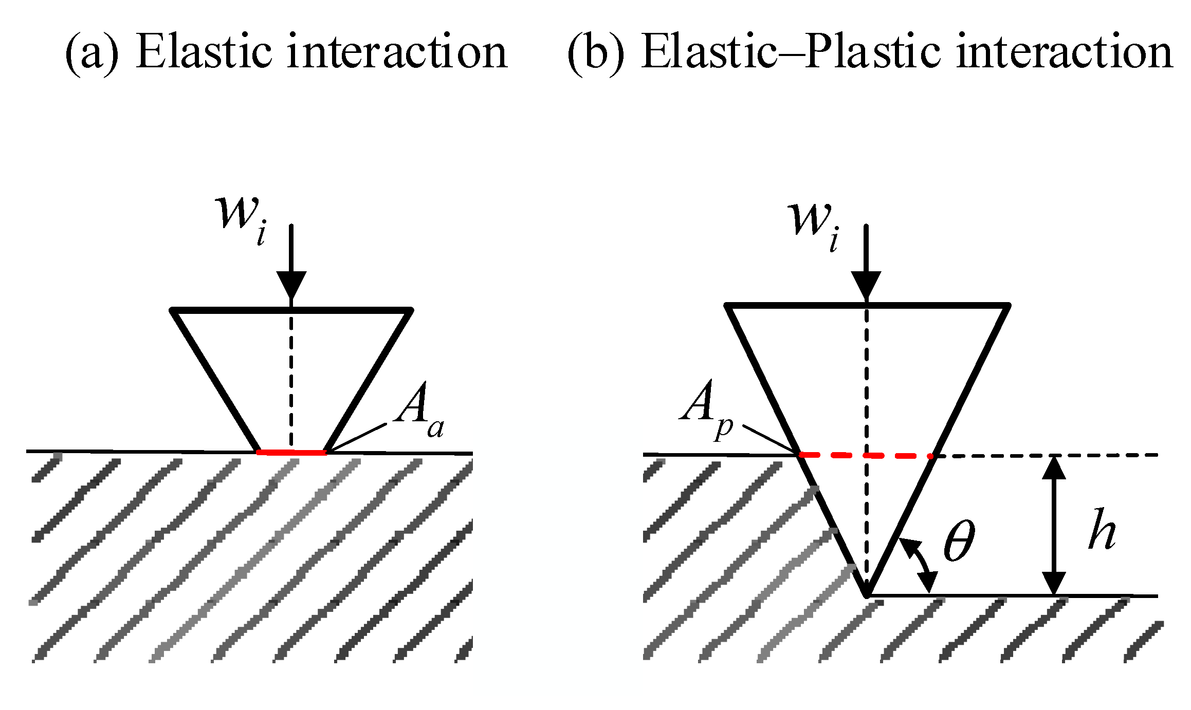
Figure 3.
The simulated rough surface (a) surface topograpy for ; (b) comparison between the generated and prescribed ACF.
Figure 3.
The simulated rough surface (a) surface topograpy for ; (b) comparison between the generated and prescribed ACF.
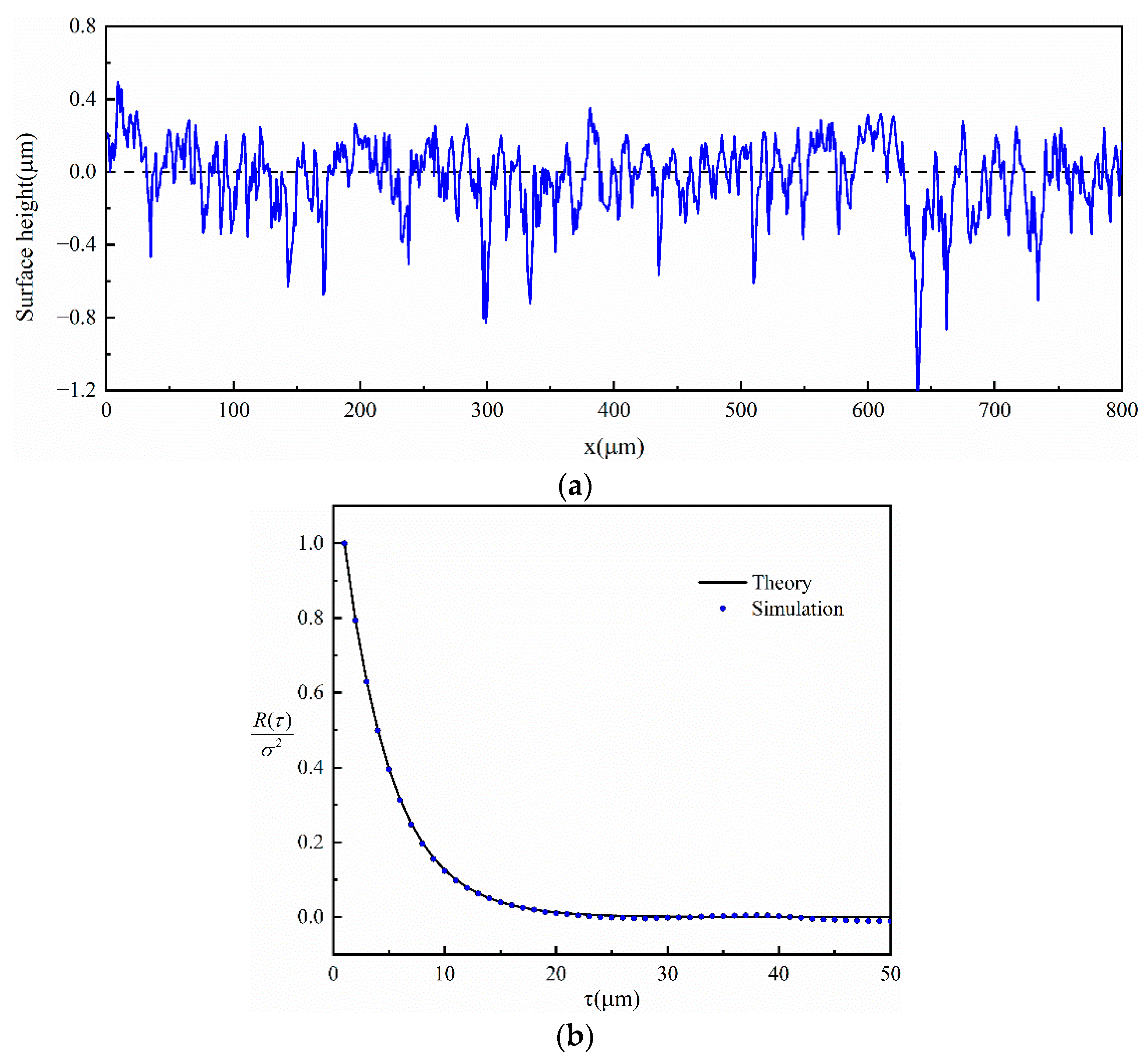
Figure 4.
Rough surface with (a) (b) .
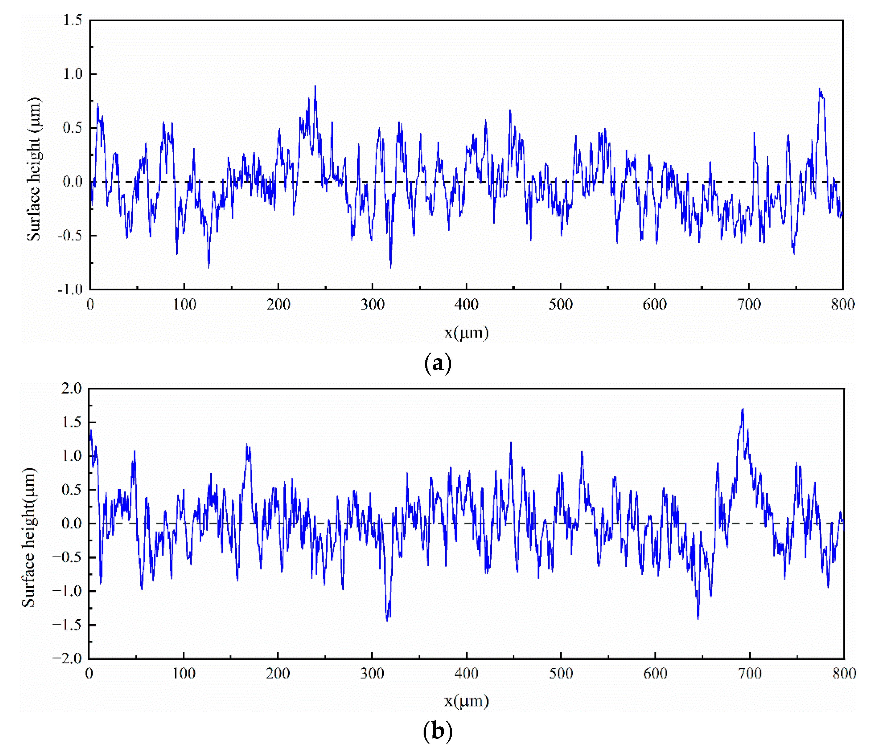
Figure 5.
Contact pressure and gap distribution under diffierent operating conditions and surface roughness: (a) ; (b) ; (c) ; (d) .
Figure 5.
Contact pressure and gap distribution under diffierent operating conditions and surface roughness: (a) ; (b) ; (c) ; (d) .
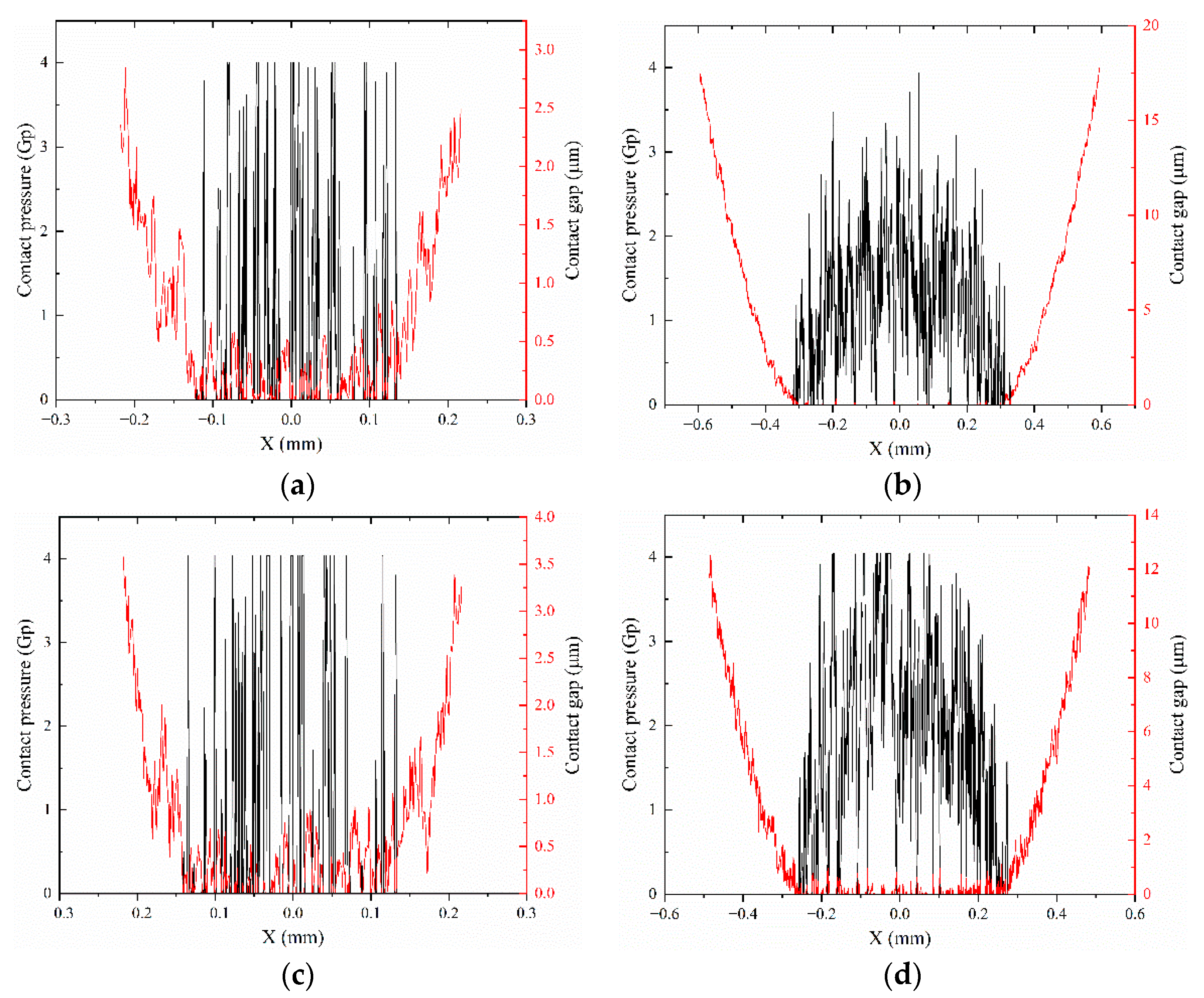
Figure 6.
Comparison of experiment results and current predictions.
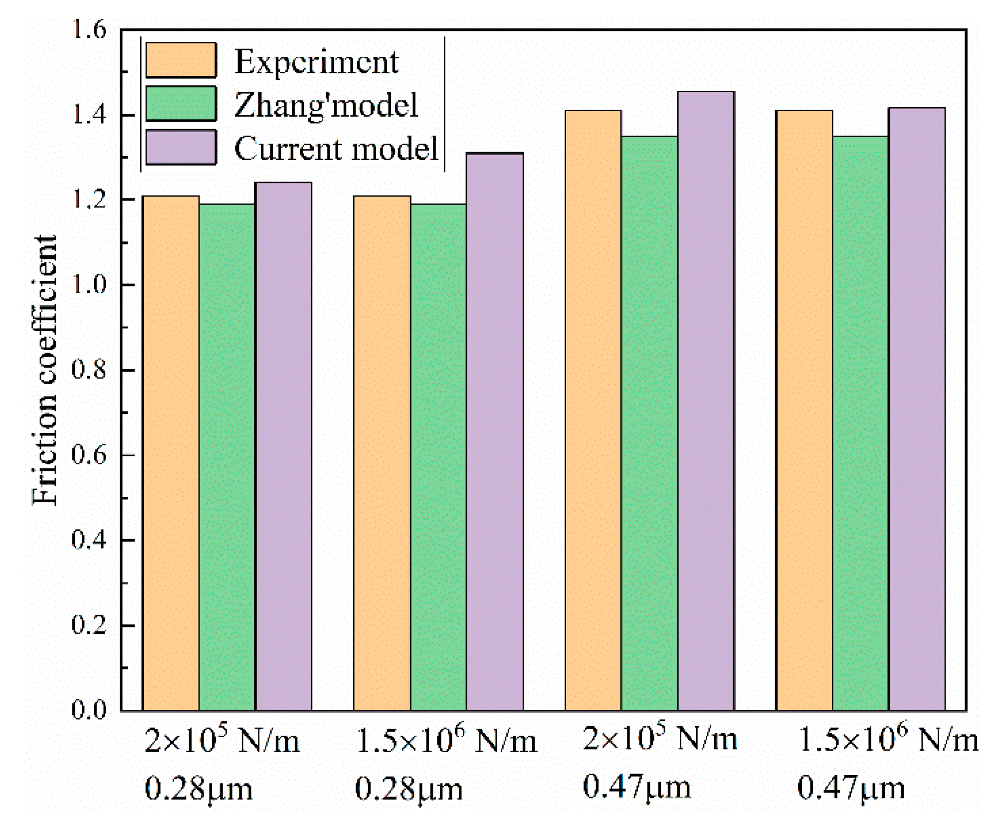
Figure 7.
Rough surface with diffierent skewness.
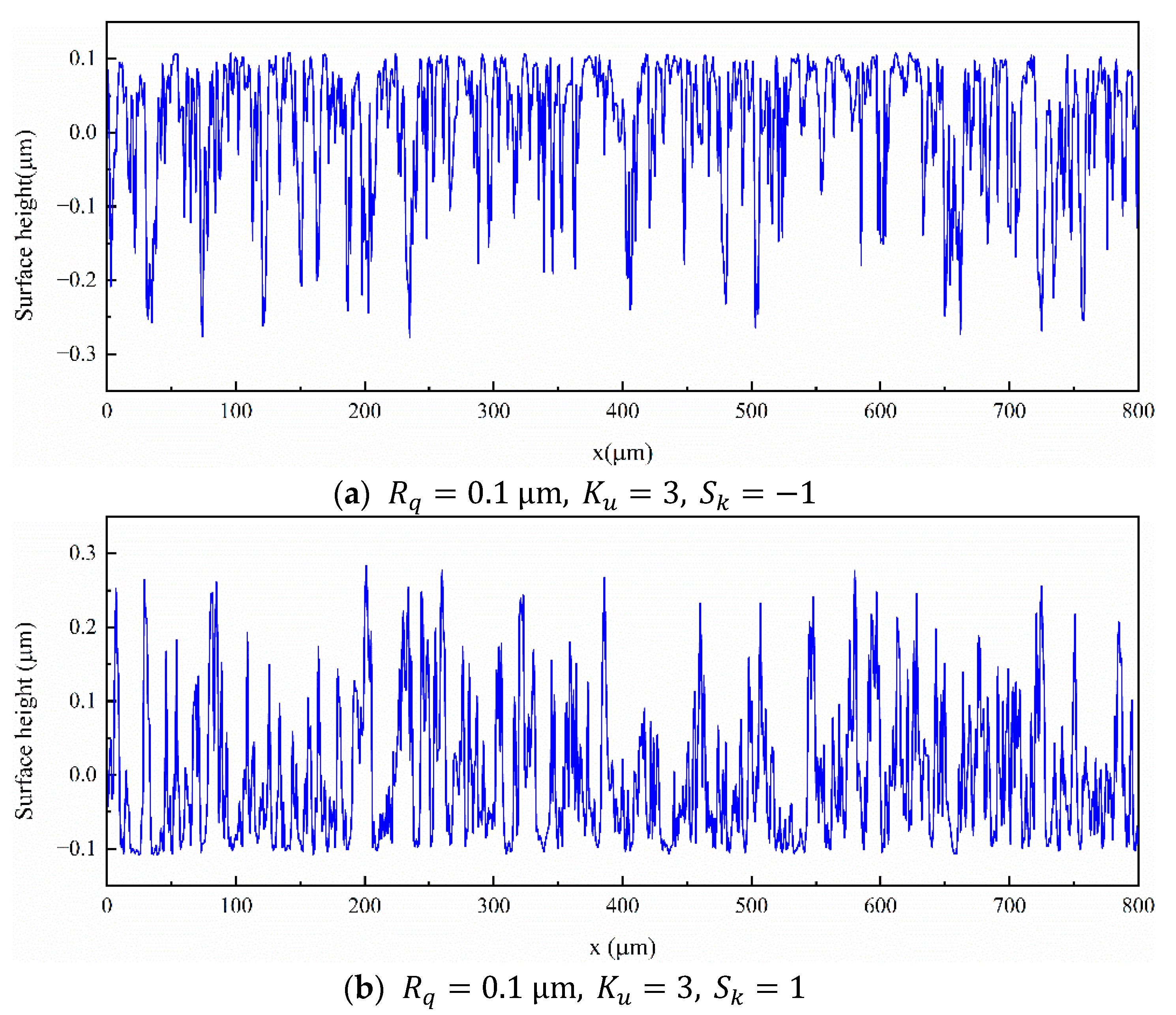
Figure 8.
The distribution of contact pressure and gap under different skewness.

Figure 9.
The effect of roughness amplitude on the friction coeficient.
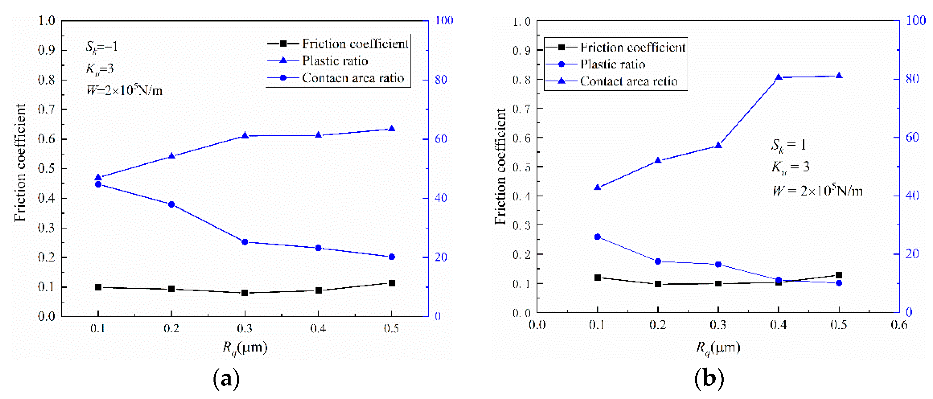
Figure 10.
The variation of average contact pressure with the roughness amplitude.
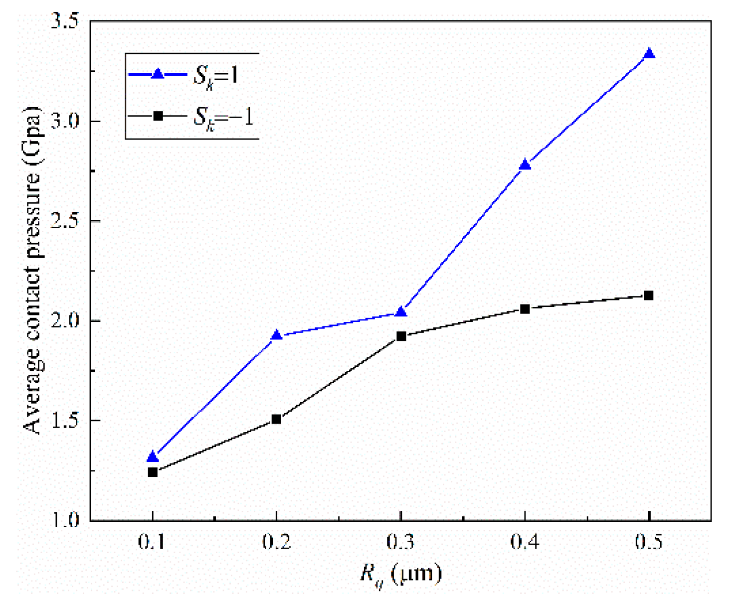
Figure 11.
Rough surface with diffierent skewness.
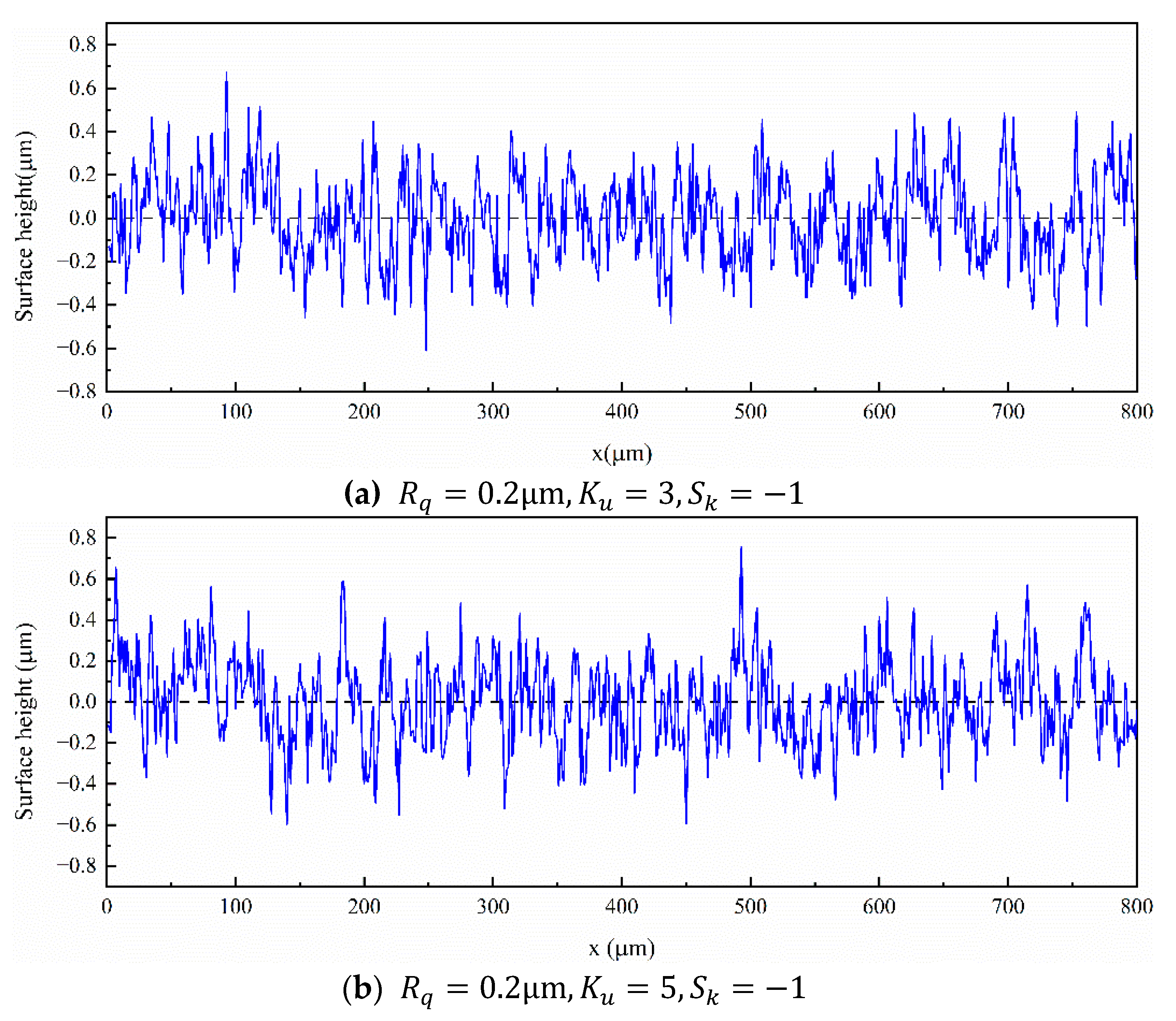
Figure 12.
Effect of kurtosis on friction coefficient, plastic ratio, and contact area ratio.
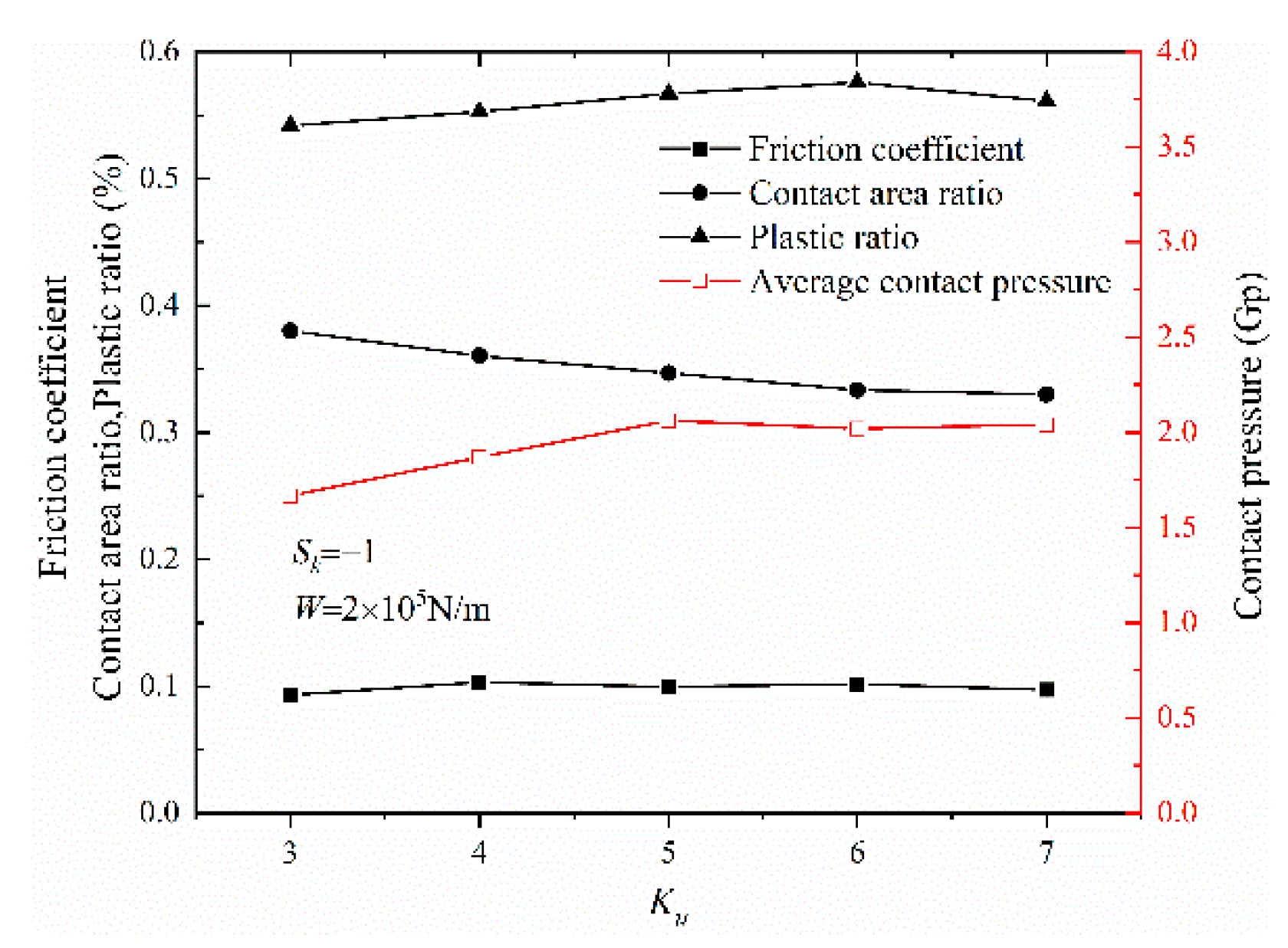
Figure 13.
Rough surface with and .
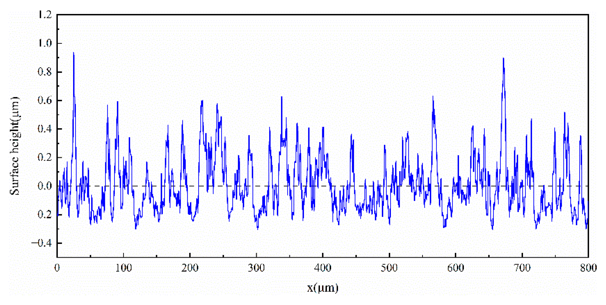
Figure 14.
Effect of load on friction coefficient, plastic ratio, and contact area ratio.
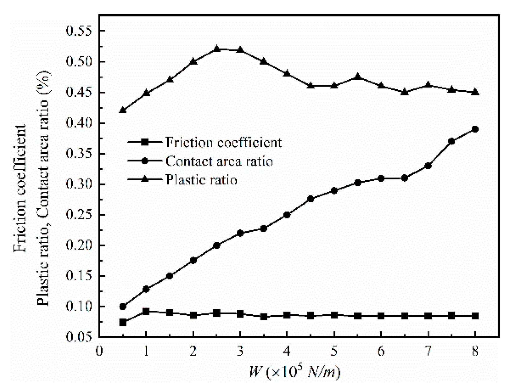
Figure 15.
Variations of average contact pressure and Herzian width with applied load.

Table 1.
Experiment operating parameters for validation.
| Applied load W (N/m) | 2 × 10⁵ and 1.5 × 10⁶ |
| Equivalent radius () | 0.0053 |
| Surface roughness | 0.28 and 0.47 |
| Equivalent elastic modulus | 2.28 × 10¹¹ |
| Hardness of rollers H (Gpa) | 4.04 |
Table 2.
Rough surfaces generated by the current method for investigating a friction coefficient.
| Surfaces | ||||
|---|---|---|---|---|
| 1–5 | 0.1–0.5 | −1 | 3 | |
| 6–10 | 0.1–0.5 | 1 | 3 | |
| 11–15 | 0.3 | −1 | 3–7 | |
| 12 | 0.3 | 0.5–8 | 1 | 4 |
Publisher’s Note: MDPI stays neutral with regard to jurisdictional claims in published maps and institutional affiliations. |
© 2022 by the authors. Licensee MDPI, Basel, Switzerland. This article is an open access article distributed under the terms and conditions of the Creative Commons Attribution (CC BY) license (https://creativecommons.org/licenses/by/4.0/).
Share and Cite
MDPI and ACS Style
Ren, J.; Yuan, H. Contact Analysis and Friction Prediction of Non-Gaussian Random Surfaces. Appl. Sci. 2022, 12, 11237. https://doi.org/10.3390/app122111237
AMA Style
Ren J, Yuan H. Contact Analysis and Friction Prediction of Non-Gaussian Random Surfaces. Applied Sciences. 2022; 12(21):11237. https://doi.org/10.3390/app122111237
Chicago/Turabian StyleRen, Jinzhao, and Huiqun Yuan. 2022. "Contact Analysis and Friction Prediction of Non-Gaussian Random Surfaces" Applied Sciences 12, no. 21: 11237. https://doi.org/10.3390/app122111237
Note that from the first issue of 2016, this journal uses article numbers instead of page numbers. See further details here.