
CFD Body Force Propeller Model with Blade Rotational Effect
Department of Systems and Naval Mechatronic Engineering, National Cheng Kung University, Tainan 70101, Taiwan
Appl. Sci. 2022, 12(21), 11273; https://doi.org/10.3390/app122111273
Submission received: 19 September 2022
/
Revised: 25 October 2022
/
Accepted: 3 November 2022
/
Published: 7 November 2022
(This article belongs to the Topic Innovation of Applied System)
Abstract
:The purpose of this study is to consider propeller geometry and blade rotation in the propeller model in a CFD code. To predict propeller performance, a body force propeller model was developed based on blade element theory and coupled with URANS (unsteady Reynolds-averaged Navier–Stokes) solver CFDSHIP-IOWA V4.5 both implicitly and interactively. The model was executed inside the flow solver every inner iteration. The grid points inside each 2D blade geometry were identified by a numerical search algorithm. To calculate the lift coefficient, the total flow velocities at 25% foil chord length were obtained using the inverse distance weighting interpolation from the RANS solution. The body forces were distributed linearly along the chord length with the maximal value located at the leading edge and zero at the trailing edge. The main achievements are: (1) for a KP505 propeller in an open water condition, the error of the thrust coefficient generally is around or less than 3%, which is a better prediction than the previous model. (2) For a behind-hull condition, the error is about 1%. (3) For an E1619 propeller in an open water condition, the error is around 6%. (4) The blade-to-blade effect and unsteady flow field between blades are sufficiently resolved by the model.
1. Introduction
Over the decades, CFD (computational fluid dynamic) has been widely applied to solve ship hydrodynamics problems. In this paper, CFD is also referred as the RANS (Reynolds-averaged Navier–Stokes) solver or URANS (unsteady RANS). CFD not only predicts the global values but also provides flow field details. The capability of the state-of-the-art CFD to consider discretized real propeller geometry behind a ship hull was demonstrated in the latest CFD workshop on ship hydrodynamics [1] (abbreviated as T2015). Three types of ship hull forms were suggested, with their own propellers and rudders: JBC (Japan Bulk Carrier), KCS, and ONRT (ONR tumblehome).
In some CFD studies, the dynamic overset grid method provides the domain connectivity information among overlapping grid blocks of ship hull and propeller. In T2015, it was implemented in OpenFOAM by Shen and Korpus [2] and the naoe-FOAM-SJTU group [3,4,5,6,7] for unstructured grids. For structured grids, Mofidi et al. [8] performed self-propulsion and course keeping for ONRT with twin propellers using overset grid in REX.
Another method is to exchange flow field data through an interface between the rotating and fixed part of grid, the so-called sliding mesh approach. Many CFD codes equip this function including commercial, academic, and open-source code, such as the following works presented at T2015: Liu et al. [9] and Qiu et al. [10] for Fluent; Bugalski et al. [11], Park and Jun [12], Kim and Jun [13], and Tenzer et al. [14] for Star-CCM+; Wu et al. [15] and d’Aure et al. [16] for FineMarine; Schuiling et al. [17] for ReFRESCO; Deng et al. [18] for ISIS-CFD; Arai et al. [19] and Abbas et al. [20] for OpenFOAM.
Regardless of whether the overset grid or sliding mesh approach is used, CFD simulations considering realistic and rotating propellers are still expensive and time-consuming. Meanwhile, several body force propeller models have been developed to save computational time and grid generation effort. Generally, propeller programs are based on the small disturbance method and potential flow theory. Thus, a numerical procedure or coupling method is required to subtract the propeller-induced velocity or obtain the effective wake from a viscous flow solution. Force distribution is predicted by propeller program and then transferred to RANS as body force, which is the source term of momentum equations. Normally, a propeller/actuator disk or a specific propeller plane is utilized to exchange those velocities and body forces between RANS and propeller code.
A body force propeller model can be a prescribed model as well, e.g., a Hough and Ordway circulation distribution [21]. Based on known propeller open water data, a given thrust and torque can be transformed to a body force distribution in CFD grids. In T2015, the model was implemented by Broglia et al. [22] in CNR-INSEAN code, Sadat-Hosseini et al. [23] for CFDSHIP-IOWA, and Lidtke et al. [24] in OpenFOAM and Star-CCM+.
In fact, body force propeller models coupled with RANS code have been under development, have a long history of use, and have been described in many publications. Until now, it has been very useful, effective, and efficient for ship applications. Stern et al. [25] coupled PUF-2 propeller code with a RANS code based on the finite analytical method. Simonsen and Stern [26] introduced a linear-induced velocity subtraction between the Yamazaki propeller model [27] and CFDSHIIP-IOWA. The propeller model was based on the lifting line method. PUF-14 code was coupled with CFDSHIP-IOWA later, as well in Chase et al. [28]. Lee and Chen [29] implemented MPUF3A propeller code inside a Chimera RANS solver to study propeller cavitation in propeller–hull interaction. Viscous nominal wake was obtained first, and then, the wake was updated by solving body forces in RANS. In the end, an effective wake for MPUF3A would be obtained. In a similar manner, Chou et al. [30] used MIT-PSF-2 propeller code in a RANS code UVW. The propeller inflow for MIT-PSF-2 is circumferentially averaged from the RANS solution. Using the circumferentially averaged inflow and updating the nominal wake to an effective one, Chen et al. [31] coupled an unsteady propeller panel code developed by Hsin [32] with Star-CCM+. Widen et al. [33] applied the blade element momentum theory in OpenFOAM to model a propeller behind a ship. Basically, those models were based on the quasi-steady assumption that the propeller rotates much faster than the ship’s advance speed. Those models only could predict time-averaged propeller flow field.
More advanced propeller models have also been proposed to distribute body force on 3D propeller geometry to consider the blade-to-blade effect or blade rotation. Kerwin et al. [34] combined a RANS solver and a vortex lattice method. The blade geometry was described by the B-spline surface for easy manipulation in design purpose. The RANS cells inside the 3D blade shape were first identified. The force per volume solved by the vortex lattice method was imposed at the cell center. The propeller panel code panMARE was utilized by Greve et al. [35] in RANS code FreSco+. A plane was located at an upstream propeller to transfer the flow velocities along the propeller’s angular and radial directions. A cell search algorithm was proposed to find the RANS cell center closest to the panel for panMARE. Later, the free surface effect was considered [36]. The singularities were distributed on the free surface geometry extracted by Fourier transform from RANS simulations with the propeller model. In the presented work, the cell was only searched in the 2D propeller plane. The side/lateral geometry of the propeller blade was neglected.
In the above-mentioned propeller models, generally, the strength of the free and bound vortex was solved inside the propeller program. The bound vortex was distributed on the propeller surface or along the foil sections. The free vortex was shedding from the trailing edge of the propeller or foil to the far downstream. Therefore, not only the propeller-induced velocity subtraction was required, but the direction of the free vortex was also assumed. However, in CFD simulations and real situations, especially when the propeller operates behind the ship hull, the free vortex is not necessarily guaranteed to be the same as assumed in the propeller program. It is much more complicated and involves the propeller tip vortex and the influence from hull–propeller–rudder interaction. To resolve this issue, a propeller model based on a quasi-steady assumption and blade element theory (BET) had been proposed [37] and has had some applications [38,39,40,41,42]. In the following discussion, it is called the “average model”, i.e., the body forces are distributed in average on the circular plane or actuator disk. The total velocity from the CFD flow solution is directly used as propeller inflow, so that the propeller-induced velocity subtraction is no longer needed. As a result, only the free vortex is solved in the propeller model. The bound vortex imbedded inside the CFD flow solution is used in the propeller computation, i.e., the propeller model and the CFD share the same bound vortex.
The purpose of the presented work is to develop the average model [37] further to consider blade rotation and more realistic geometry. It is still based on BET using total velocity and coupled with the RANS solver CFDSHIP-IOWA V4.5 implicitly and interactively. The innovation of the proposed propeller model is summarized as follows. The blade geometry in the 2D propeller plane is constructed by chord length, pitch, and skew distribution. The grid points inside the blade’s leading and trailing edges are identified by a numerical search algorithm. The propeller’s local thrust and torque are calculated using the lift and drag coefficients. The total velocities at 25% of chord length along foil section are provided via the inverse distance weighting interpolation from a RANS solution. The body force is distributed linearly along the chord length with a peak value at the leading edge and a value of zero at the trailing edge. Several actual applications of the proposed model are conducted successfully. A five-bladed KP505 propeller is simulated in open water for advance coefficient J = 0.3 to 1.0. A grid independence test is conducted for J = 0.5, 0.7, and 0.8. The predicted thrust and torque coefficients show good agreement with experimental values. The unsteady flow phenomena of the blade-to-blade effect and vortex shedding are simulated successfully. The E1619 propeller in open water and KP505 propeller behind KCS (KRISO container ship) hull are investigated for one J.
2. Numerical Methods
2.1. CFDSHIP-IOWA
The simulations were performed by the URANS (unsteady Reynolds-averaged Navier–Stokes) solver CFDSHIP-IOWA V4.5 [43] to model the viscous flow field around ship and propeller complex geometries, ship motions and unsteady propeller rotational flow. A multi-block structured grid with overset grid capability was used. The solver featured semi-captive, full-6DOF (degree of freedom), parallel, and high-performance computing (HPC) capabilities. The non-dimensional governing equations in the solver were [41]:
where t is time, u is the vector form of velocity field, is the grid velocity for considering ship motions, and PS is the pressure term. The gravity term is included in PS. is the source term, which will represent the body forces produced by propeller model (Section 2.2 and Section 2.3). is the effective Reynolds number defined by ship speed U, ship length L, kinematic viscosity of fluid , and turbulent viscosity solved by the SST (shear stress transport) k–ω turbulence model without wall function [44]:
The SST k–ω model is widely used in ship hydrodynamics application, and its robustness and global reliability had been concluded at T2015 [45] and the previous workshop [46].
To model the free surface, the governing equation of the single-phase level set method [47] is:
where is the level set function or distance function. The free surface is defined along the iso-surface of , and the undisturbed free surface is located at z/L = 0. indicates that the grid is full of water. In the region of , i.e., air, URANS is not solved.
The numerical methods to discretize and solve the above-mentioned governing equation are based on the second-order finite-difference method. The Euler backward method is used for the time derivatives, the upwind method is used for the convection term, and the central difference is used for the diffusion term. The velocity and pressure field were coupled by the projection method. The details have been addressed in [41].
2.2. Average (Body-Force Propeller) Model
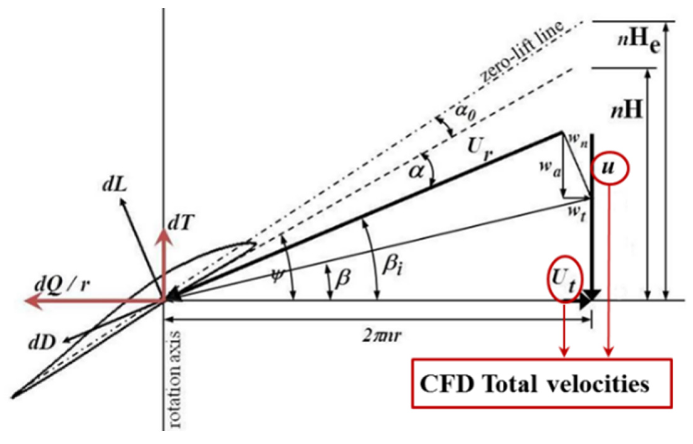
In the average model [37], the flow total velocities (u/U, v/U, and w/U) provided by the URANS solver were directly input into the inflow to calculate the lift and drag on each blade element as shown in Figure 1. The lift coefficient CL was obtained by
CD = 0.01.
The local thrust dT and torque dQ, at each grid point inside the propeller disk (cylindrical block) are calculated from the CL and CD on the corresponding blade element. Propeller pitch is considered to calculate α. Chord length is needed when computing dT and dQ from CL and CD. Finally, the axial and tangential body forces (fbx, fbθ), i.e., force per volume, are obtained as:
As implied in Equation (7) of [37] and Equation (8), the model is based on the average effect of dT and dQ among N blades, propeller rotation perimeter 2πr at certain radius r, and thickness of the propeller actuator disk Δx.
The average effect, i.e., the quasi-steady assumption, is useful for ship applications because propellers rotate at high speeds in many scenarios such as self-propulsion in calm water or waves and seakeeping and manoeuvring problems. The momentum equations in the URANS solver are solved along with those body forces as the source terms. The six components of total propeller forces and components are considered in the equations of motions in a 6DOF solver. The flow field is solved in an earth-fixed coordinate, 6DOF motions are solved in ship-fixed coordinate, and the propeller model computation is in the propeller-shaft coordinate. Thus, several coordinate transformations are required in the code.
2.3. Rotating Blade (Body Force Propeller) Model
The numerical procedure to consider 2D blade geometry and rotation is explained as follows:
2.3.1. Blade Geometry Generation (2D Outline)
According to the non-dimensional chord length C/, pitch P/, and skew distribution along the propeller radius, which are generally provided by the propeller offset table, the propeller geometry on an axial plane (x: shaft axis) or a y–z plane can be constructed. For an N-bladed propeller, the mid-chord line would be:
herein, = 1, 2 …, N. Here, k′ = 1 is to produce mid-chord line. The leading and trailing edge can then be generated from the mid-chord line:
At certain time t, the coordinate transformation due to blade rotation is:
in which n is propeller rotation rate (RPS, revolution per second).
If a 3D model of propeller geometry is available, the leading and trailing edge points and relative to the propeller center (0,0,0) can be extracted first. Next, the propeller skew (), pitch P, and chord length C can be calculated by Equations (19)–(21), respectively. Finally, the propeller blade outline can be constructed by following the previous Equations (9)–(15).
2.3.2. Cell Search Algorithm
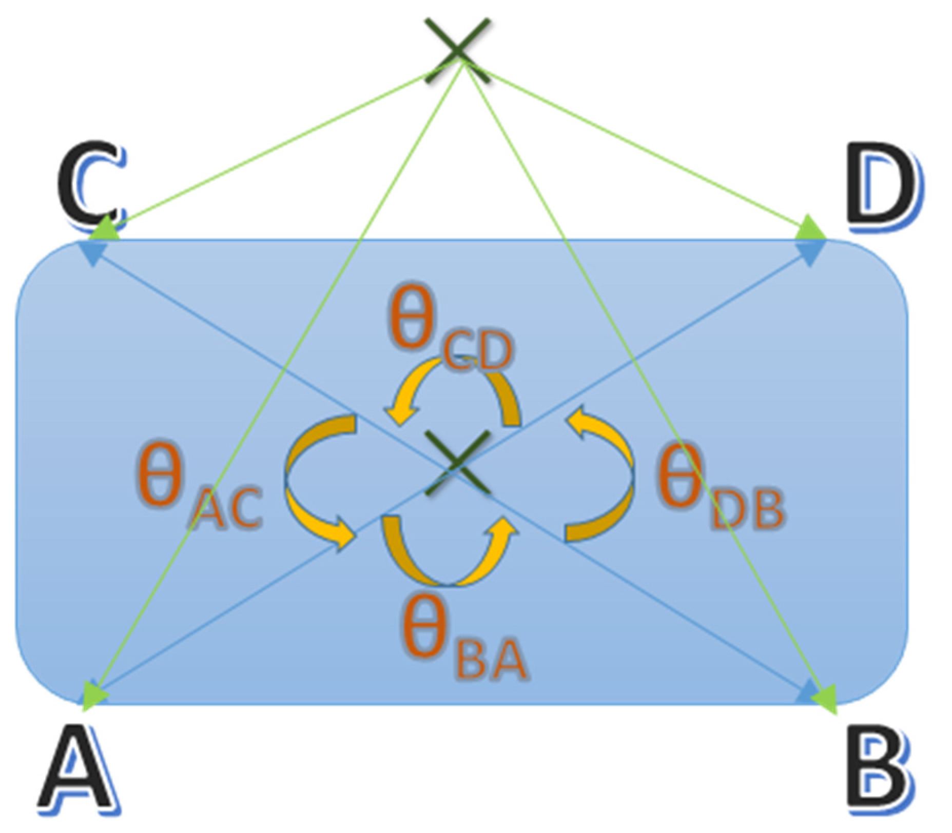
Searching for and identifying the RANS grids inside the propeller geometry outline is required. In this study, the search algorithm is based on dot product and angle summation. If the propeller geometry outline from Section 2.3.1 is split into several convex cells, the vector between the RANS grid point and each cell edge point can be defined as shown in Figure 2. By calculating the dot product, the angle between a pair of two adjacent vectors is obtained. There are four pairs of vectors corresponding to four angles. If Equation (22) is satisfied, the RANS grid point is inside the cell (propeller outline).
θAC + θCD + θDB + θBA = 2π,
θAC + θCD + θDB + θBA < 2π.
Instead, if Equation (23) is satisfied, the RANS grid point is outside the cell (propeller outline).
2.3.3. Blade Element Theory at ¼ Chord Position
Once the RANS grid point is identified inside one blade, the propeller computation is conducted on the corresponding foil section/blade element at that propeller radius. The total velocities are obtained for the 25% chord position , which is the usual location of the aerodynamic center for a foil section.
can be generated by Equations (3) and (4) using k’ = 0.5. The cell search algorithm in Section 2.3.1 is performed again to locate the RANS grid points surrounding the point , such as for points A, B, C, and D as shown in Figure 2. Accordingly, the total velocities at are obtained by the inverse distance weighting interpolation from the velocities on point A, B, C, and D:
where is the distance between and grid point. The grid point A, B, C, and D are assigned to i = 1, 2, 3, 4, respectively. The power parameter p is a positive real number, and is set as 1.51294159474 which is a common value used in CFD-SHIPIOWA V4.5.
The main part of propeller computation is the same as in the average model in Section 2.2. The only difference in this case is the body force distribution. In the rotating blade model, the linear body force distribution is specified along the chord length C with the maximal value at leading edge, and a value of zero at the trailing edge. If is at x’/C portion of the chord length C, the body forces are distributed axially and tangentially as below:
Figure 3 illustrates the linear distribution of the axial and tangential body force.
2.4. Computational Domain and Boundary Conditions
Two simulation conditions are considered in the presented study. The first condition is the simulation of a single propeller in open water conditions. Two different propellers, KP505 and E1619, are simulated in open water using the same CFD setup and grid system. The second simulation condition is the behind hull condition, i.e., the simulation of a KCS model ship hull appending an operating KP505 propeller simplified by the propeller models (Section 2.2 and Section 2.3). The computational domain and boundary conditions for the two conditions are explained separately in the following Section 2.4.1 and Section 2.4.2.
2.4.1. Open Water Propeller Test
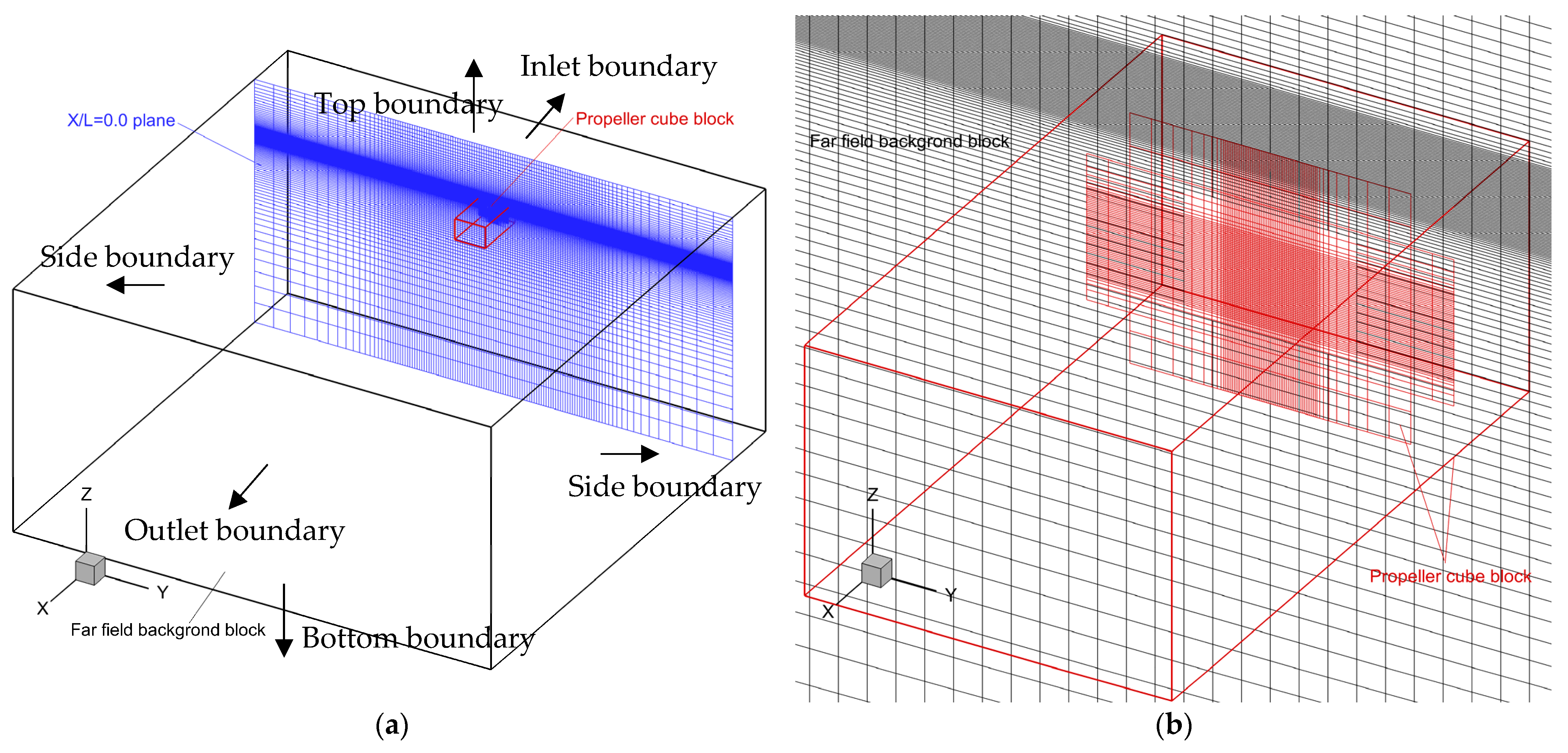
The overset grid system and computational domain are the same as in the previous work [39] for the wave condition with the deepest propeller immersion depth. Here, it is only for the calm water condition, but the free surface is considered. Although only the propeller is simulated here, for the further application of the behind hull condition, the CFD computational domain is non-dimensionalised by the model length of KCS: L = Lpp (length between perpendiculars) = 3.2 m. The domain size is −0.24 < x/L < 1.75 from upstream to downstream, −1 < y/L < 1 from side to side, and −0.79 < z/L < 0.22 from top to bottom. The propeller plane is at x/L = 0.0. The domain consisted of two overset grid blocks: the propeller cube and far-field background, as shown in Figure 4. Inside the propeller cube, the grid number is 50 × 50 on the x/L = 0 plane to cover the propeller diameter. Table 1 shows the grid number detail. The total grid number is 3.5 M (million). The uniform inflow boundary condition is specified on the inlet, the exit condition for the outlet, the zero-gradient condition on both sides, and the far-field condition on the top and bottom face of the domain. The non-dimensional inflow velocity U is set as 1, and the open water test for different J is conducted by adjusting propeller rotation rate n. The mathematical formulae for the boundary conditions are listed in Table 2 and specified on the boundaries indicated in Figure 4a. There is no solid surface in the open water test here because no physical propeller exits inside the domain. The body force propeller models simplify the propeller. The grid system and CFD setup are the same for the rotating blade and average propeller model, and for KP505 and E1619 propeller.
2.4.2. Propeller behind Hull Condition
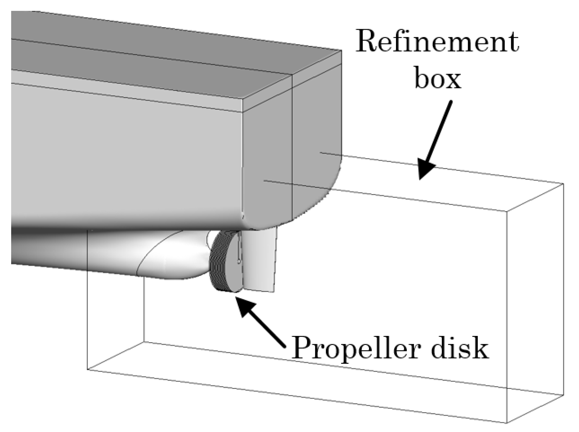
The propeller KP505 behind the KCS hull with a rudder in calm water is also tested in the presented work. A propeller disk (cylinder grid block) is required for applying both the average and rotating blade body force propeller models. The same CFD grid system including the propeller disk, and the setup is shared between the two propeller models. Figure 5 explains the computational domain and boundary conditions detailed in Table 2 accordingly. Figure 6 shows the propeller disk is attached on the ship stern bulb with the propeller boss and in front of the rudder. The disk has a central tunnel, which is also the propeller boss surface. The rotating hub velocity, i.e., propeller rotational velocity, is specified on the inner surface of the disk central tunnel. In this section, the ship vertical motions including heave and pitch are considered to predict the sinkage and trim in CFD simulation using dynamic overset grid performed by Suggar. An identical grid system was used in the previous study [41] as well.
The entire grid system is composed of nine blocks to describe the complicated geometry: starboard and portside for hull, cover (hull top), stern (including shaft tube and dummy boss), and rudder (attached under transom) and one background. The total grid number is around 13 M (million). To capture turbulence, the minimum size of the grid approximately is 1 × 10⁻⁶ normal to the solid surface corresponding to y+ < 1. Fine grids are generated in the x-direction near the ship and the z-direction near the free surface to capture and maintain the propagating waves.
3. Results
3.1. KP505 Propeller in Open Water Test
KP505 is a five-bladed propeller with a skew angle designed for a KCS container ship. The main propeller dimensions are available on the T2015 workshop website [1]. The geometric details are shown in Figure 7 for the technical drawing and Table 3 for the offset table. Because the offset table was available, the 2D geometry outline was extracted using Equations (3)–(9).
3.1.1. Thrust and Torque Coefficient
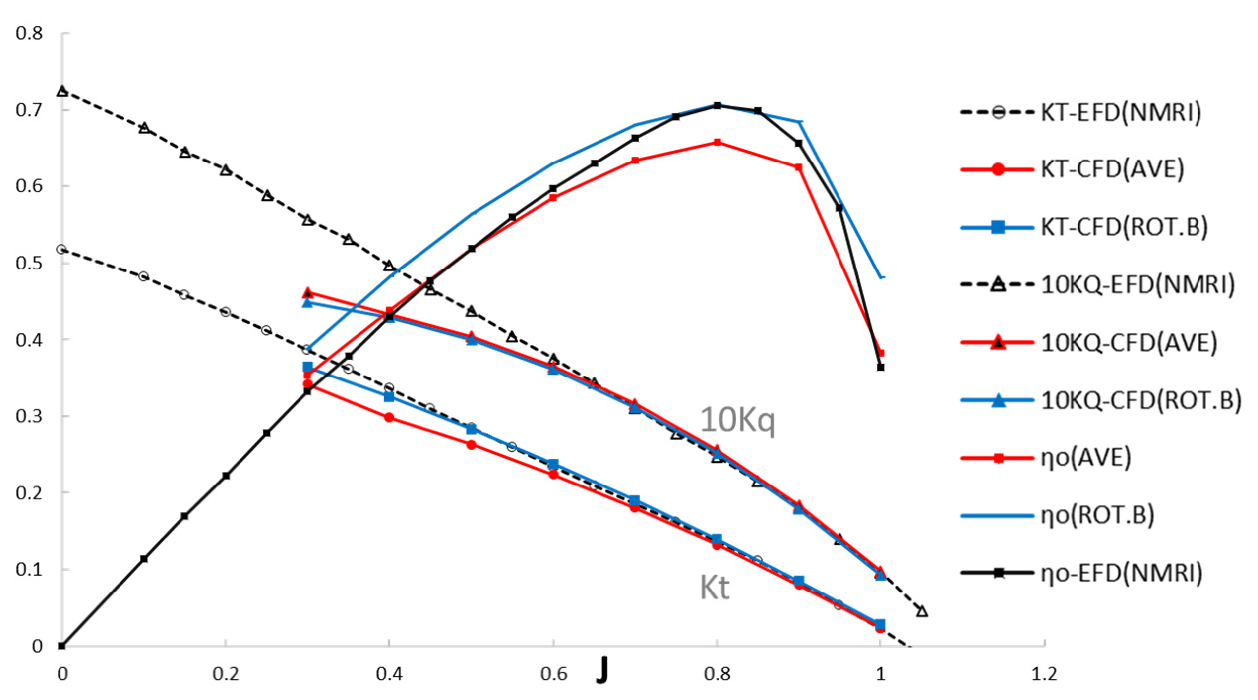
As shown in Figure 8, the propeller thrust and torque coefficient (KT, KQ) predicted by the proposed rotating blade model were compared with the average model result and experimental data provided by NMRI (National Maritime Research Institute, Tokyo, Japan) for the T2015 workshop [1]. The result of both propeller models shows good agreement with the experiment, especially for the high J (advance coefficient) region. The KT values were from J = 0.3 to 1.0 in the experiment, and the rotating blade and average models are listed in Table 4. In the table, the error E%D for the two models are included as well, and evaluated as follows:
wherein D represents the experimental data and S is the simulation value. For the rotating blade model, the KT in low J (J 0.5) is under-predicted and the KT is over-predicted at high J (J > 0.5). The absolute error |E%D| is less than or around 3%, except for at the two extreme values of J, i.e., 0.3 and 1.0. The smallest error is less than 1%, at J = 0.5. Zero error is expected between J = 0.5 and 0.6. From low to high J excluding J = 1.0, the average model provides under-predicted errors increasing from around 3% to more than 10%. The |E%D| of the average model is generally larger than that of the rotating blade model (except for at J = 0.7 and 1.0).
For J = 0.1, KT is close to zero, leading to prediction difficulty. Furthermore, it is easy to obtain larger error value because the very small D value is the denominator of Equation (30). In the following discussion for KT, J = 0.1 will not be included.
As J decreases, the KT and KQ of both models predict lower values and deviate more clearly from the experimental data. Especially at low J value, the performance of both models is limited by the blade element theory which cannot consider foil section geometry. Equation (5) may not be suitable for high-angle attack conditions. Because CD is assumed as a small constant, CL is the dominated component which is computed in the current propeller computation. With the consideration of 2D blade geometry, more realistic body force distribution and blade-to-blade interaction, the rotating blade model can provide a larger CL, producing better KT prediction. In contrast, the average model is a highly simplified model, which is merely an actuator disk. In other words, due to lack of the foil geometry consideration, the CL of the average model is generally too low. The KT of the rotating body force is around 7% larger than the average model one, on average.
The KQ values of J = 0.3 to 1.0 of the experiment, rotating blade, and average model are listed in Table 5. In the table, the error E%D for the two models are included as well and evaluated as in Equation (3). Both models show a similar trend and error level. As J decreases, |E%D| becomes worse. The error raises close to 10% when J 0.5. This issue is caused by the assumption of constant CD = 0.01, i.e., Equation (6). With low values of J corresponding to a high-angle attack condition, the real CD is larger than 0.01, so both models predict lower a lower value KQ. With high values of J, e.g., J > 0.6, CD = 0.01 is very close to a real situation with a small angle of attack. Consequently, both models could provide considerably small |E%D| with under- or over-prediction.
However, the rotating blade model does not perform better than the average model for KQ. For only J = 0.7, 0.8, and 0.9, the rotating blade model provides better error, and the |E%D| of J = 0.9 is the lowest amongst all data. In contrast to KT, The KQ of the rotating body force is around 2% smaller (on average) than that of the average model. For propeller torque computation, the foil section drag is more relevant, but CD only can be assumed as a constant in both propeller models currently. Because CD = 0.01 is only applied inside the blade region, the KQ is all smaller for the rotating blade model. Instead, CD = 0.01 was specified on the whole propeller disk area in the average model, so that the KQ is all larger.
3.1.2. Grid Independence Test
Based on the Section 3.1.1 result, the condition J = 0.5, 0.7, and 0.8 are selected to check grid independency of the propeller model and CFD method of the presented work. J = 0.5 has the minimal KT error, which is under-predicted less and around 1% in Table 4. J = 0.7 has the minimal KQ error, which is over-predicted nearly only 0.2% in Table 5. The KT and KQ predictions are performed in balance at J = 0.8. with error about 1.7–1.8%. The averaged absolute error for J = 0.8 is 1.75% which is second lowest among all J values. It is only slightly higher than the error of J = 0.7 (1.57%), because the KQ error of J = 0.7 is really low.
The analysis of grid independence and uncertainty here is based on the verification and validation theory suggested by ITTC 7.5-03-01-01 guideline [48]. A different grid size and density are required. The grid in the previous section and Table 2 is served as medium grid, and then the grid number is increased by (Ni, Nj, Nk) to become a fine grid. Reducing the grid number, the coarse grid is built by (Ni, Nj, Nk). Finally, the total grid number is 1.2 M (1,217,280) and 9.8 M (9,777,246) for the coarse and fine grid, respectively. The simulation values of fine, medium, and coarse grid are assigned in this section as S1, S2, and S3, respectively. The grid dependence test results for KT and KQ are presented in Table 6 and Table 7, respectively. All S2 values are the same as the S values in Section 3.1.1. The D value and E%D calculation follows Section 3.1.1 as well.
The grid independence is judged by the RG value, which is calculated as below:
Grid independence is accomplished for |RG| < 1, meaning that the value difference between the medium and fine grid is smaller than the difference between medium and coarse grid. As shown in Table 5 and Table 6, all CFD results achieve grid independence, i.e., as the grid number increases, the results converge. Monotonic convergence (M.C.) is reached for 0 < RG < 1, and oscillating convergence (O.C.) is reached for −1 < RG < 0. Except for the result that the KQ of J = 0.5 is M.C., the other CFD results satisfy the O.C. condition.
For M.C., the grid uncertainty (UG) is estimated by the generalized Richardson extrapolation with factor of safety suggested by [48]. For O.C., UG is simply evaluated from the minimal and maximal values among three different grid results [48]:
which is presented as percentage of D in Table 5 and Table 6. The result achieving a UG > |E%D| of S1 would be considered as valid. As a consequence, for a KT of J = 0.5 and 0.8 and a KQ of J = 0.7 and 0.8, validation is achieved. Once grid convergence is confirmed, it strongly depends on if S1 could produce small enough error, i.e., how accurate the simulation can reach as the grid grows finer. For J = 0.8, KT and KQ both are validated. This indicates that the current CFD method and setup is the most suitable for the J = 0.8 condition.
In actuality, for KT of J = 0.7, the UG is only slightly smaller than |E%D| of S1 with a less than 1% difference. Thus, the comparisons between the CFD results themselves are only slightly less confident than comparisons with the experiment. This is also because the KT is slightly deviated from D somehow from S2 to S1, i.e., when refining the grid from medium to fine grid. The |E%D| increase is very small, also less than 1%. In fact, if comparing UG with |E%D| of S2, it can be considered to be validated, i.e., UG > |E%D| of S2.
For KQ of J = 0.5, a very small UG value is found, which reflects that S1 and S2 are extremely close to each other. Thus, the confidence level for the comparison of the CFD results themselves is much higher than that of comparison with the experiment. As Table 6 reveals, E%D rises to close to 9% as the grid number increases from S3 to S2, and then to S1. This is related to the fact that constant CD = 0.01 is unsuitable for low J condition, previously discussed. A larger drag coefficient would increase propeller torque in low J condition because the high angle of attack. A severe increase in error can be observed in Figure 8 and Table 5 as well. Future development of the propeller model, e.g., a more sophisticated CD correction, is required.
3.1.3. Body Force Distribution
Figure 9 presents a comparison of axial body force (fbx) distribution for J = 0.8 between the rotating blade and average model result. As mentioned in the previous section, in the rotating blade model, the body force is maximal along the leading edge and zero along the trailing edge. The distribution is linear. The figure also shows the cells (marked by the thin lines) identified inside the propeller blade outline (marked by the thick black lines). For the average model, the body force distribution is axisymmetric on a disk inside the propeller radius.
3.1.4. Propeller Wake Field
Figure 10 shows the velocity profile behind the propeller for J = 0.8. The flooded contour is the axial velocity, and the vector field includes both lateral and vertical velocities. For the rotating blade model, the blade-to-blade effect to the flow field is clearly observed at x/L = 0.005 (Figure 10a). In the radial direction, the high-velocity region is located around r/R = 0.4 to 0.8. It is not axisymmetric along the circumferential direction. The velocity drops slightly between two adjacent blades, i.e., the trailing edge of the current blade and the leading edge of the next blade. The area shrinks as well. The flood contour near the blade leading edge has a clear concave shape. However, at just slightly downstream (e.g., x/L = 0.01 in Figure 10b) the flow field of rotating blade model becomes almost axisymmetric. The contour pattern is almost identical to the average model one in Figure 10c, which is steady, i.e., it would not change by time.
In Figure 11 (J = 0.8) and Figure 12 (J = 0.6), the free surface waves caused by the propeller excitement have a very small amplitude, because the propeller immersion depth is in deep water. In the comparison of both propeller models, the wave amplitude of the rotating blade model at a specific timepoint is smaller than that of the average model at the same timepoint. It decays more obviously and faster in the far downstream region as well. This phenomenon is more obvious for J = 0.6, and the waves become more laterally scattered downstream in the rotating blade model. This is because the body forces are only distributed on the blades, producing discontinuous influence in the lateral direction on the free surface. Comparing the different J values, the lower J shows a higher axial velocity on the propeller plane, a larger wave amplitude, and a shorter effective pitch indicated by the streamlines.
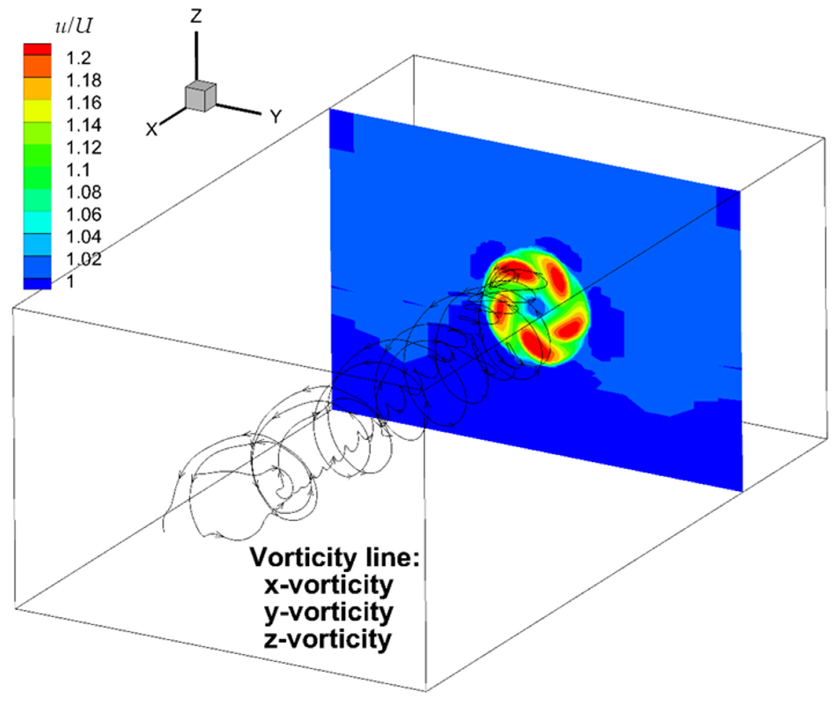
Figure 13 plots the 3D vorticity lines to observe the vortex shedding behind the propeller KP505. The propeller rotational flow with (high frequency) tip vortex shedding is clear in the figure. Additionally, on the propeller plane each blade tip corresponds with a lower velocity area outside the propeller radius.
3.2. E1619 Propeller in Open Water Test
In contrast to KP505 and Section 3.1, this section will investigate a propeller with a short chord length, i.e., a small EAR (expanded blade area ratio) and available for a 3D geometry model instead of an offset table. The seven-bladed and highly skewed submarine propeller E1619 was chosen. The main particulars are shown in Table 8. Its 3D model was provided by INSEAN (Italian Ship Model Basin), and the 2D geometry outline was extracted using Equations (10)–(15). The CFD setup and grid system are exactly the same as the one used in Section 3.1. This is also proof of the high flexibility of the presented propeller model; it is convenient and easy to switch between not only two body force propeller models but also different propeller geometries.
For J = 0.8, the CFD using the presented blade rotating blade propeller model predicts KT = 0.205. Against the experimental KT = 0.218, the error E%D is around 6% under-predicted. Figure 14 illustrates the axial velocity distribution directly following the propeller plane. To compare the result in Figure 14, please refer the Figure 4.13 on p. 36 in [49]. The area of high velocity behind each blade body is described well for real propeller simulations (CFDSHIP-IOWA using overset grid) [49], LDV experiments [49], and the proposed rotating blade propeller model. The velocity drops between the two blades are captured as well.
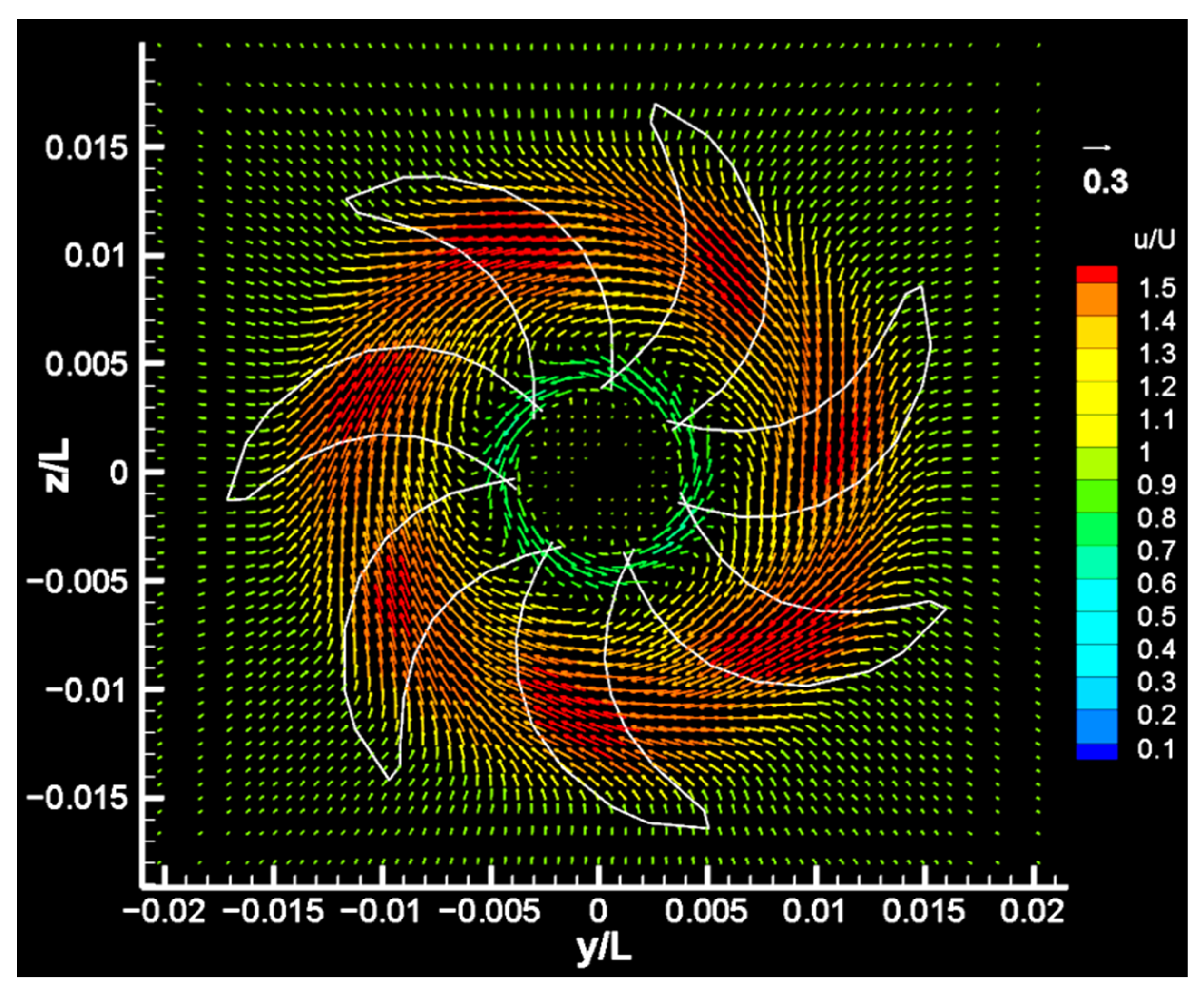
However, when using the rotating blade propeller model the lower velocity area outside the propeller radius next to each blade tip is not clear for the E1619 propeller (Figure 14). In contrast, it is clearer for the KP505 propeller in Figure 15. It can also be observed clearly in the real propeller simulation [49] and the LDV experiment [49]. Because of the small chord length and expanded blade area ratio of E1619, the grid numbers across its narrow tip are less than can be covered by that of the KP505. The grid number is insufficient to adequately resolve the flow field phenomena. This issue will be investigated by a finer grid in the future.
The propeller downstream vector field was presented in Figure 16 for the rotating blade model. Due to lack of an experimental vector field, the PIV measurement behind a submarine with an X-rudder [50,51], e.g., Figure 13 in [51], could be used a reference for a brief comparison. A submarine is a slender body and the rudder is outside the propeller radius. Both results show that the vector directions are twisted in front of the blade’s leading edge in the propeller’s rotational direction. The vectors pointing to the propeller center change to the propeller’s rotational direction around 0.7 R. The axial velocity increases behind the blade body.
3.3. KP505 Propeller behind KCS Hull
Table 9 shows the results of the propeller thrust coefficient KT for the experiments and CFD using the average and the rotating blade body force model for the behind-hull condition. The propeller rotational speed is 16.3 RPS and was obtained using a self-propulsion test in a towing tank at Osaka University for a 3.2 m long ship model at Froude number Fr = 0.26 [41]. Both models under-predicted the KT by around 1%. The rotating blade result was obtained by restarting from the average model result to save computational time. The time step is required to be very small for the rotating blade model to obtain a converged and stable result. In the presented work, the time step for the average model was around 0.0055 s, while it was 0.00022 s for the blade rotating model (around 1.3 degrees of propeller rotation).
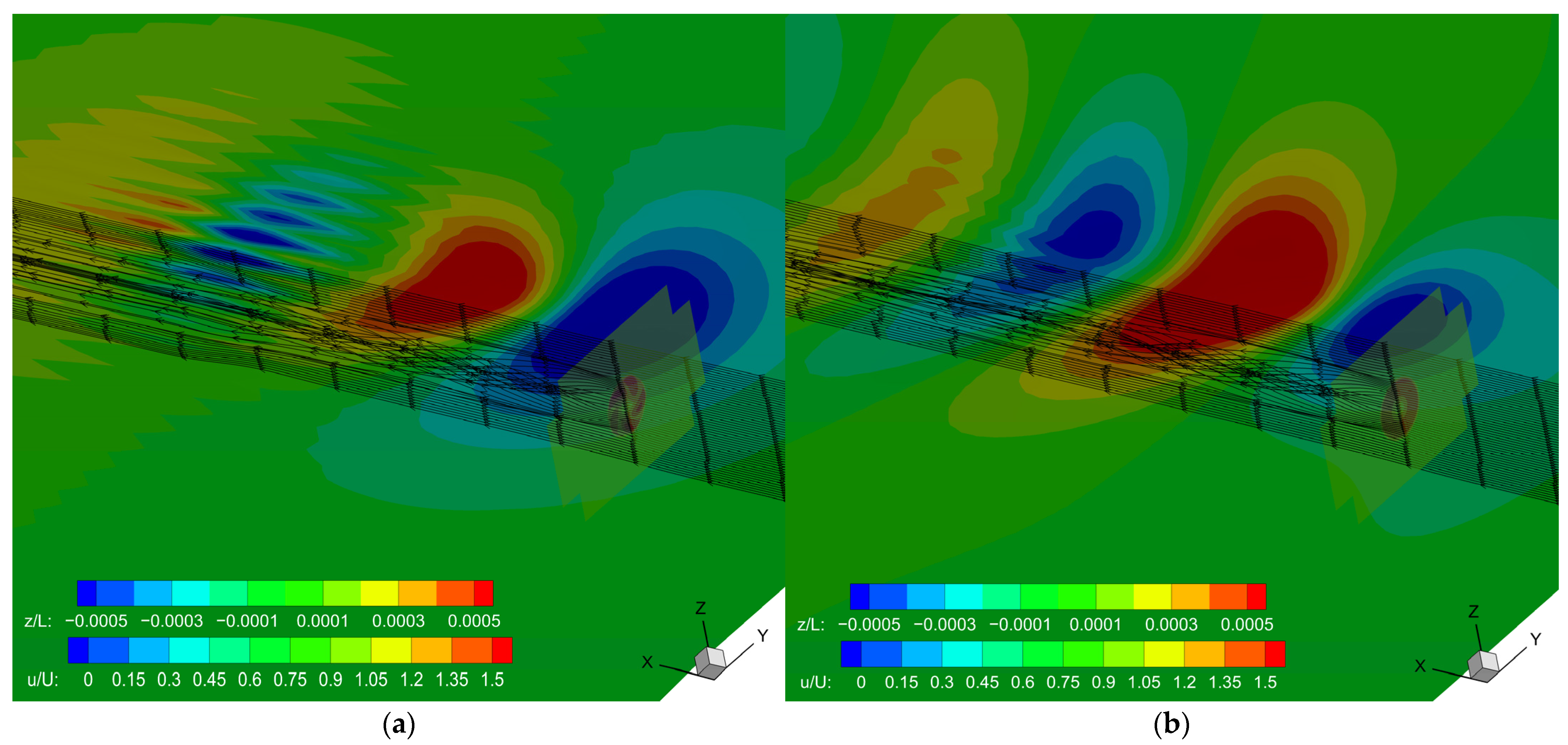
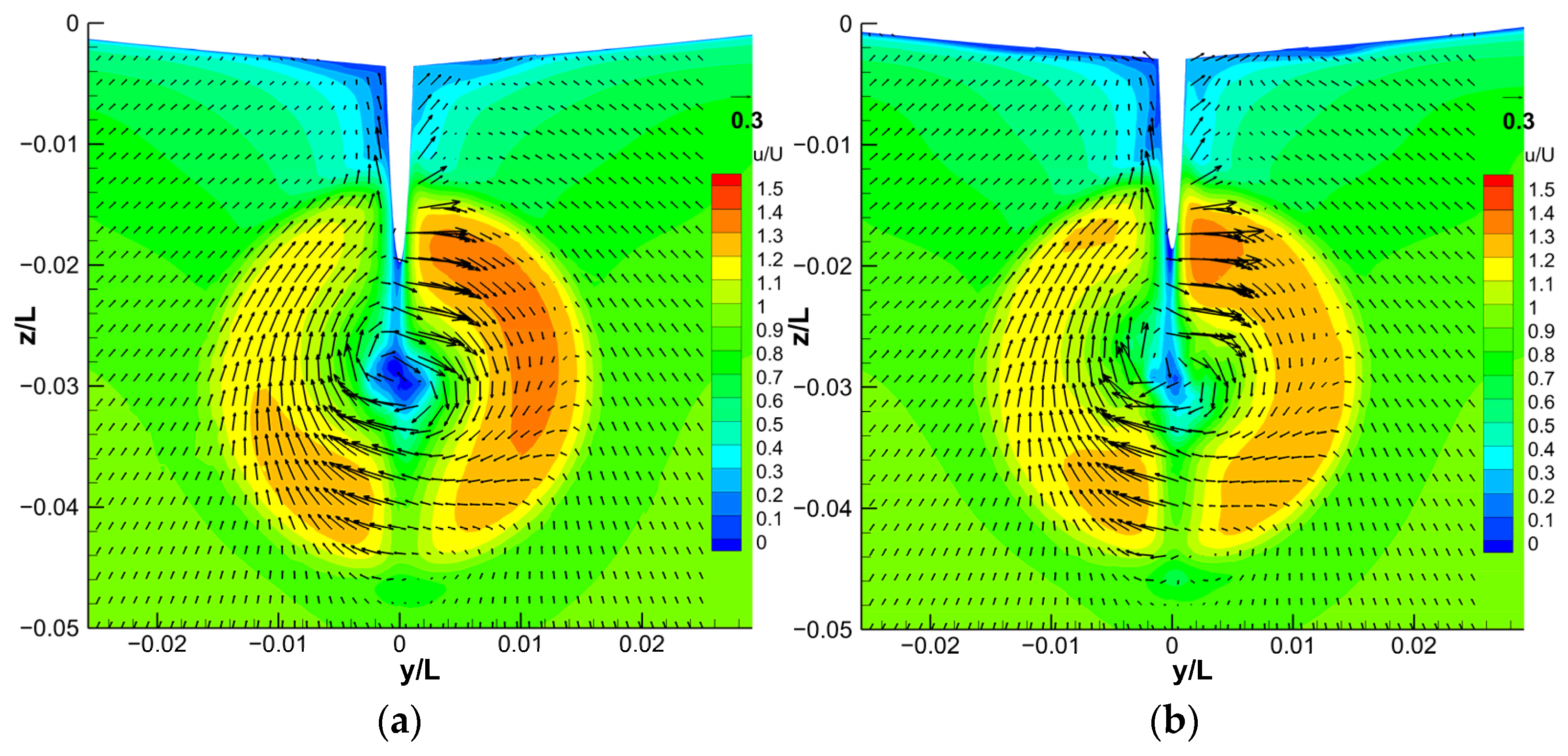
Figure 17 presents the flow field plotted by the axial velocity contour (u/U) and vector field for cross flow (v/U, w/U) after the rudder, i.e., x/L = 1.025. U is the ship model speed. x/L = 0.0 is at the ship FP (front perpendicular). Figure 17a is the PIV (particle image velocimetry) measurement. Figure 17b is the result of the CFD using the average model. Figure 17c is the result of the CFD using the rotating blade model. The three results show a similar flow pattern. Because of the right-rotating propeller, high axial velocity is located mainly in the starboard. The highest u/U values in (a) and (c) are in a more similar position near z/L = −0.04, where is the lower part of the starboard side flow field. The highest u/U in Figure 17b is a longer band region in the middle of the starboard side flow field. The clockwise-rotating flow is interfered by the rudder in the middle, so the portside cross flow was twisted to form an upward jet and it is pointing downward in the starboard. The hub vortex is separated, becoming two cores as well: the portside core is in the lower position and starboard core is in the higher position. A vortex was induced by outer upward flow and starboard downward cross flow around (y/L, z/L) = (0.01, −0.02). This is the corner of the high u/U contour (in yellow color, i.e., u/U = 1.2–1.3). In Figure 17a,c, the corner shape is sharper than the one in Figure 17b. Basically, the flow field away from the propeller is nearly steady even though the propeller rotational flow is unsteady. This can also be seen in Figure 18 for the flow field between the propeller and rudder, i.e., x/L = 0.99. The propeller plane is at x/L = 0.9825 (the ship AP is at x/L = 1.0 and the ship FP is at x/L = 0). In Figure 18, both models show a similar flow field pattern, but the average model has a larger high-axial-velocity area in the starboard side.
In conclusion, for the downstream steady flow field behind the propeller, the above comparison indicates that the rotating blade model result is closer to the experimental model, because it considers a more realistic geometry. Comparing it with the average model, the body forces of the rotating blade model are distributed only on the blade with lower thrust prediction (Table 9) such that the distribution of high velocity downstream is more scattered and has lower values.
When the wake field is near the propeller, the rotating blade model reveals an unsteady phenomena. The x/L = 0.985 section is right behind the propeller plane (x/L = 0.9825). Figure 19 indicates the average model result. Because of the right-rotating propeller, the region of high axial velocity is observed in the starboard side. This is a time-averaged and steady flow field. Instead, the results of the rotating blade model plotted in Figure 20 for different blade positions show an unsteady flow field changing by time (the force computation is still under a quasi-steady assumption). In Figure 20, the flow field around every 18 degrees of the index blade rotation is plotted. Four time instants are divided, from the index blade near approximate 0 degrees (tip pointing up vertically) to 54 degrees. The index blade at 72 degrees is the next blade at 0 degrees again because it is a five-bladed propeller (360/5 = 72 degrees). At a different time instant, the high-axial-velocity area still occurs in the starboard side but at a lower position, i.e., the fourth quadrant (Figure 19). As the blade rotates into the fourth quadrant one after another, high axial velocity is generated on the blade area inside the quadrant and moves along with the blade until it leaves the quadrant.
4. Conclusions
The rotating blade propeller model has been developed successfully based on the blade element theory and using total velocity from RANS solution. A cell search algorithm was implemented to identify the RANS grid points inside the 2D propeller geometry. The propeller computation is based on the 25% chord length position along a foil section. The body forces were distributed linearly across the chord line with a maximal value at the trailing edge and a value of zero at the linear edge. Simulations for the KP505 and E1619 propellers in open water, and the KP505 propeller behind the KCS hull were successfully conducted.
For KP505 propeller, the results showed good agreement with experimental data and had a small error mainly in high-load conditions. The propeller thrust coefficient was predicted well by the rotating blade model. For the KP505 propeller in open water conditions, the absolute error of the thrust coefficient was generally around or less than 3%. The lowest error was less than 1% under-prediction for the advance coefficient J = 0.5. Prediction of torque coefficient was not as successful because of the constant drag coefficient assumption. Grid independence was achieved for J = 0.5, 0.7, and 0.8. The CFD result was also validated for J = 0.8, i.e., the comparison between the converged CFD result and the experiment was more confident than the comparison between the CFD results themselves.
In open water and behind-hull conditions, the unsteady phenomena and blade-to-blade effect occur only when the propeller wake field is very close to the propeller. This also supports the conclusion that the body force propeller model can be applied to many ship applications.
For KP505 appended and operating behind the KCS hull in calm water, the thrust coefficient of the rotating blade model error was about 1%. For the downstream wake field, the rotating blade model provided a steady result closer to the experimental result than the average model’s result. The high-velocity distribution was more scattered and had a lower value because the body forces were only distributed on the blades and the thrust was under-predicted. For the wake field right after the propeller, the unsteady phenomena were obvious. As the blades rotated into the fourth quadrant in sequence, the starboard area of high axial velocity appeared on the incoming blade and moved together with the blade until the blade left the quadrant. For the average model, the area of high axial velocity simply remained on the starboard side constantly and did not change over time.
For E1619 in open water condition, the error was under-predicted by around 6%. The high-velocity areas behind each blade and velocity drops between the two blades are sufficiently captured by the rotating blade model. However, the area of lower velocity outside the propeller tip was not clear, because the grid number was not sufficient around the narrow blade tip.
The contribution of the presented study is the implementation of the total velocity concept and blade rotation with 2D blade geometry in a CFD body force propeller model. Discretized real propeller simulation is still time consuming. Grid generation is difficult and complicated. The rotating blade body force model will be a great alternative for considering unsteady flow field phenomena and blade-to-blade effect. Only an additional cylinder disk is required. Grid generation is easy with a lower grid number. The same grid system can be applied for different propellers. In this study, it was also proven that the propeller model works in open water and behind-hull conditions.
In future work, the propeller computation will be developed further to solve the vortex lattice on the grid cell found on propeller plane. Additionally, the linear body force distribution will be replaced with data from literature or a more realistic curve to represent the pressure difference distribution on a foil. Furthermore, side/lateral geometry will be included to consider propeller chamber and thickness. To do so, a 3D cell search algorithm will be required to identify the RANS grid point inside the body volume of the real propeller. Using this method, the body force will be able to be distributed in an arbitrary 3D shape such as a realistic propeller geometry.
Funding
The authors would like to thank the Ministry of Science and Technology (MOST) for their support of the project [MOST 111-2221-E-006-153]. It was thanks to the generous patronage of the MOST that this study was smoothly performed.
Institutional Review Board Statement
Not applicable.
Informed Consent Statement
Not applicable.
Data Availability Statement
Not applicable.
Conflicts of Interest
The authors declare no conflict of interest.
Nomenclature
| AP | Ship after perpendicular [-] |
| α | Angle of attack (AOA) |
| β | Closure coefficient in turbulence model [-] |
| C | Chord length [m] |
| CL | Lift coefficient [-] |
| CD | Drag coefficient [-] |
| D | Experimental data [-] |
| Propeller diameter [m] | |
| dT | Local thrust [N] |
| dQ | Local torque [N∙m] |
| Δx | Thickness of propeller actuator disk [m] |
| E%D | Error [-] |
| fbx | Axial body force [N] |
| fbθ | Tangential body forces [N] |
| FP | Ship front perpendicular [-] |
| i | Grid point index in one RANS cell [-] |
| J | Propeller advance coefficient [-] |
| k | Turbulence kinetic energy [m2⋅s−2] |
| k1 | Empirical correction for finite blade width [-] |
| k’ | Coefficient to produce mid- or 25% chord line [-] |
| KT | Propeller thrust and torque coefficient [-] |
| KQ | Propeller torque coefficient [-] |
| L | Model ship length (=Lpp) [m] |
| Lpp | Length between perpendiculars (=L) [m] |
| n | Propeller rotation rate [rps, s−1] |
| Which propeller blade in number order [-] | |
| υt | Turbulence viscousity [m2⋅s−1] |
| N | Number of propeller blades [-] |
| Ni | Grid number in axial direction [-] |
| Nj | Grid number in lateral direction [-] |
| Nk | Grid number in vertical direction [-] |
| M | Million [-] |
| ω | Specific turbulence dissipation rate [s−1] |
| p | Power parameter [-] |
| P | Pitch [m] |
| PS | Pressure [N⋅m2] |
| ϕ | Level set function [-] |
| r | Radial coordinate (position) in cylinder/propeller coordinate [m] |
| Distance between foil 25% chord position and grid point [m] | |
| R | Propeller radius [m] |
| Re | Reynolds number [-] |
| Effective Reynolds number [-] | |
| RG | Grid independence indicator [-] |
| S | Simulation value [-] |
| S1 | Simulation value of fine grid [-] |
| S2 | Simulation value of medium grid [-] |
| S3 | Simulation value of coarse grid [-] |
| Source term (vector) [N⋅m−3] | |
| t | Time [s] |
| Propeller skew angle | |
| u | Axial flow velocity [m/s] |
| u | Vector form of velocity field [m/s] |
| Grid velocity [m/s] | |
| Axial velocity at grid point [m/s] | |
| Axial velocity at foil 25% chord position [m/s] | |
| U | Inflow or inlet velocity, i.e., ship speed [m/s] |
| UG | Grid uncertainty [-] |
| v | Lateral flow velocity [m/s] |
| Lateral velocity at grid point [m/s] | |
| Lateral velocity at foil 25% chord position [m/s] | |
| w | Vertical flow velocity [m/s] |
| Vertical velocity at grid point [m/s] | |
| Vertical velocity at foil 25% chord position [m/s] | |
| Weighting function [-] | |
| x | Axial position/direction in Cartesian coordinate [m] |
| x’ | Position along foil chord length [m] |
| Axial position of blade leading edge [m] | |
| Foil 25% chord position in axial coordinate [m] | |
| Axial position of blade trailing edge [m] | |
| y | Lateral position/direction in Cartesian coordinate [m] |
| Lateral position of blade leading edge [m] | |
| Foil 25% chord position in lateral coordinate [m] | |
| Lateral position of blade trailing edge [m] | |
| y+ | Non-dimensional thickness of the first layer grid from solid surface [-] |
| z | Vertical position/direction in Cartesian coordinate [m] |
| Vertical position of blade leading edge [m] | |
| Foil 25% chord position in vertical coordinate [m] | |
| Vertical position of blade trailing edge [m] |
References
- Tokyo 2015 Workshop on CFD in Ship Hydrodynamics. Available online: https://t2015.nmri.go.jp/index.html (accessed on 4 December 2015).
- Shen, Z.; Korpus, R. Numerical simulations of ship self-propulsion and maneuvering using dynamic overset grids in OpenFOAM. In Proceedings of the Tokyo 2015 CFD Workshop, Tokyo, Japan, 2–4 December 2015. [Google Scholar]
- Liu, X.; Zhao, W.; Wan, D. Verification and Validation for CFD Simulation of KRISO Container Ship. In Proceedings of the Tokyo 2015 CFD Workshop, Tokyo, Japan, 2–4 December 2015. [Google Scholar]
- Sun, T.; Yin, C.; Wu, J.; Wan, D. Numerical Computations of Resistance for Japan Bulk Carrier in Calm Water. In Proceedings of the Tokyo 2015 CFD Workshop, Tokyo, Japan, 2–4 December 2015. [Google Scholar]
- Wang, J.; Liu, X.; Wan, D. Numerical prediction of free running at model point for ONR Tumblehome using overset grid method. In Proceedings of the Tokyo 2015 CFD Workshop, Tokyo, Japan, 2–4 December 2015. [Google Scholar]
- Wu, J.; Yin, C.; Sun, T.; Wan, D. CFD-Based Numerical Simulation of Self-Propulsion for Japan Bulk Carrier. In Proceedings of the Tokyo 2015 CFD Workshop, Tokyo, Japan, 2–4 December 2015. [Google Scholar]
- Yin, C.; Wu, J.; Sun, T.; Wan, D. A numerical study for self-propelled JBC with and without energy saving device. In Proceedings of the Tokyo 2015 CFD Workshop, Tokyo, Japan, 2–4 December 2015. [Google Scholar]
- Mofidi, A.; Castro, A.; Carrica, P.M. Self-Propulsion and Course Keeping of ONR Tumblehome in Calm Water and Waves. In Proceedings of the Tokyo 2015 CFD Workshop, Tokyo, Japan, 2–4 December 2015. [Google Scholar]
- Liu, D.; Zhang, Z.; Zhao, F. The Numerical Simulation on the Interaction between Propeller and JBC Hull with and without ESD. In Proceedings of the Tokyo 2015 CFD Workshop, Tokyo, Japan, 2–4 December 2015. [Google Scholar]
- Qiu, G.; Wu, C.; Zhao, F.; Wang, W. CFD Simulation of Self-Propulsion ONRT Model in Head Wave. In Proceedings of the Tokyo 2015 CFD Workshop, Tokyo, Japan, 2–4 December 2015. [Google Scholar]
- Bugalski, T.; Wawrzusiszyn, M.; Hoffmann, P. Numerical Simulations of the KCS-Resistance and Self-Propulsion. In Proceedings of the Tokyo 2015 CFD Workshop, Tokyo, Japan, 2–4 December 2015. [Google Scholar]
- Park, S.H.; Jun, J.H. Numerical Simulations of KCS and ONRT Using STAR-CCM+. In Proceedings of the Tokyo 2015 CFD Workshop, Tokyo, Japan, 2–4 December 2015. [Google Scholar]
- Kim, G.H.; Jun, J.H. Numerical Simulations for Predicting Resistance and Self-Propulsion Performances of JBC Using OpenFOAM and STAR-CCM+. In Proceedings of the Tokyo 2015 CFD Workshop, Tokyo, Japan, 2–4 December 2015. [Google Scholar]
- Tenzer, M.; Sigmund, S.; Lantermann, U.; el Moctar, B. Prediction of Ship Resistance and Ship Motion in Calm Water and Regular Waves Using RANSE. In Proceedings of the Tokyo 2015 CFD Workshop, Tokyo, Japan, 2–4 December 2015. [Google Scholar]
- Wu, Q.; Feng, X.M.; Yu, H.; Wang, J.B.; Cai, R.Q. Prediction of Ship Resistance and Propulsion Performance on a Bulk Carrier. In Proceedings of the Tokyo 2015 CFD Workshop, Tokyo, Japan, 2–4 December 2015. [Google Scholar]
- d’Aure, B.; Mallol, B.; Hirsch, C. Resistance and Seakeeping CFD Simulations for the Korean Container Ship. In Proceedings of the Tokyo 2015 CFD Workshop, Tokyo, Japan, 2–4 December 2015. [Google Scholar]
- Schuiling, B.; Windt, J.; Rijpkema, D.; van Terwisga, T. Computational Study on Power Reduction by a Pre-Duct for a Bulk Carrier. In Proceedings of the Tokyo 2015 CFD Workshop, Tokyo, Japan, 2–4 December 2015. [Google Scholar]
- Deng, G.; Leroyer, A.; Guilmineau, E.; Queutey, P.; Visonneau, M.; Wackers, J.; del Toro Llorens, A. Verification and Validation of Resistance and Propulsion Computation. In Proceedings of the Tokyo 2015 CFD Workshop, Tokyo, Japan, 2–4 December 2015. [Google Scholar]
- Arai, Y.; Takai, M.; Kawamura, T. Ship Flow Computations Using OpenFOAM with Rotating Propeller. In Proceedings of the Tokyo 2015 CFD Workshop, Tokyo, Japan, 2–4 December 2015. [Google Scholar]
- Abbas, N.; Kornev, N. Computations of the Japan Bulk Carrier Using URANS and URANS/LES Methods Implemented into OpenFOAM Toolkit. In Proceedings of the Tokyo 2015 CFD Workshop, Tokyo, Japan, 2–4 December 2015. [Google Scholar]
- Hough, G.R.; Ordway, D.E. The generalized actuator disc. Theor. App. Mech. 1965, 2, 317–336. [Google Scholar]
- Broglia, R.; Dubbioso, G.; Zaghi, S. Numerical Computation of the JBC with and without Energy Saving Device. In Proceedings of the Tokyo 2015 CFD Workshop, Tokyo, Japan, 2–4 December 2015. [Google Scholar]
- Sadat-Hosseini, H.; Sanada, Y.; Stern, F. ONRT Coure Keeping and Turning Circle Maneuvering in Regular Waves. In Proceedings of the Tokyo 2015 CFD Workshop, Tokyo, Japan, 2–4 December 2015. [Google Scholar]
- Lidtke, A.; Lakshmynarayanana, A.P.; Camilleri, J.; Badoe, C.E.; Banks, J.; Phillips, A.B.; Turnock, S.R. RANS Computations of Flow around a Bulk Carrier with Energy Saving Device. In Proceedings of the Tokyo 2015 CFD Workshop, Tokyo, Japan, 2–4 December 2015. [Google Scholar]
- Stern, F.; Kim, H.T.; Zhang, D.H.; Toda, Y.; Kerwin, J.; Jessup, S. Computation of Viscous Flow around Propeller-Body Configurations: Series 60 CB=0.6 ship model. J. Ship Res. 1994, 38, 137–157. [Google Scholar] [CrossRef]
- Simonsen, C.; Stern, F. RANS Maneuvering Simulation of Esso Osaka with Rudder and a Body-Force Propeller. J. Ship Res. 2005, 49, 98–120. [Google Scholar] [CrossRef]
- Yamazaki, R. On the Propulsion Theory of Ships on Still Water—Introduction. In Memoirs of the Faculty of Engineering; Kyushu University: Kyushu, Japan, 1968; Volume 27, pp. 187–220. [Google Scholar]
- Chase, N.; Thad, M.; Carrica, P.M. Overset Simulation of a Submarine and Propeller in Towed, Self-propelled and Maneuvering Conditions. In Proceedings of the 29th Symposium on Naval Hydrodynamics (SNH), Gothenburg, Sweden, 26–31 August 2012. [Google Scholar]
- Lee, S.K.; Chen, H.C. The Influence of Propeller/Hull Interaction on Propeller Induced Cavitating Pressure. In Proceedings of the 15th International Ocean and Polar Engineering Conference (ISOPE), Seoul, Korea, 19–24 June 2005. [Google Scholar]
- Chou, S.K.; Hsin, C.Y.; Chen, W.C.; Chau, S.W. Simulating the Self-Propulsion Test by a Coupled Viscous/Potential Flow Computation. In Proceedings of the 8th International Symposium on Practical Design of Ships and Other Floating Structures (PRADS), Shanghai, China, 16–21 August 2001. [Google Scholar]
- Chen, K.C.; Hsin, C.Y.; Lee, C.P. Evaluation of the Effect of Ship Motion on Propeller Performance. In Proceedings of the 6th Pan Asian Association of Maritime Societies (PAAMES) meeting and Advanced Maritime Engineering Conference (AMEC), Hangzhou, China, 28–30 October 2014. [Google Scholar]
- Hsin, C.Y. Development and Analysis of Panel Methods for Propellers in Unsteady Flows. Ph.D. Thesis, Massachusetts Institute of Technology, Cambridge, MA, USA, 6 September 1990. [Google Scholar]
- Winden, B.; Badoe, C.; Turnock, S.R.; Phillips, A.B.; Hudson, D.A. Self Propulsion in Waves Using a Coupled RANS-BEMt Model and Active RPM Control. In Proceedings of the 16th Numerical Towing Tank Symposium (NuTTS’13), Mulheim, Germany, 2–4 September 2013. [Google Scholar]
- Kerwin, J.E.; Keenan, D.P.; Black, S.D.; Diggs, J.G. A Coupled Viscous/Potential Flow Design Method for Wake-Adapted Multi-Stage, Ducted Propulsors Using Generalized Geometry. Trans.-Soc. Nav. Archit. Mar. Eng. 1994, 102, 23–56. [Google Scholar]
- Greve, M.; Wöckner-Kluwe, K.; Abdel-Maksoud, M.; Rung, T. Viscous-Inviscid Coupling Methods for Advanced Marine Propeller Applications. Int. J. Rotating Mach. 2012, 2012, 743060. [Google Scholar] [CrossRef] [Green Version]
- Greve, M.; Abdel-Maksoud, M. Potential Theory Based Simulations of Unsteady Propeller Forces Including Free Surface Effects. In Proceedings of the 4th International Symposium on Marine Propulsors (SMP15), Austin, TX, USA, 31 May–4 June 2015. [Google Scholar]
- Tokogz, E.; Wu, P.C.; Yokota, S.; Toda, Y. Application of new body-force concept to the free surface effect on the hydrodynamic force and flow around a rotating propeller. In Proceedings of the 24th International Ocean and Polar Engineering Conference (ISOPE), Busan, Korea, 15–20 June 2014. [Google Scholar]
- Wu, P.C.; Tokgoz, E.; Okawa, K.; Toda, Y. Computation and Experiment of Propeller Performance and Flow Field around Self-propelled Model Ship in Regular Head Waves. In Proceedings of the 31st Symposium on Naval Hydrodynamics (SNH), Monterey, CA, USA, 11–16 September 2016. [Google Scholar]
- Wu, P.C.; Tokgoz, E.; Takasu, S.; Shibano, Y.; Toda, Y. Application of Propeller Model in Waves near Free Surface in Open Water and Behind-Hull Condition. J. Jpn. Soc. Nav. Archit. Ocean Eng. 2016, 23, 160–166. [Google Scholar]
- Truong, T.; Wu, P.C.; Kishi, J.; Toda, Y. Improvement of Rudder-Bulb-Fin System in Ship and Propeller Wake Field of KVLCC2 Tanker in Calm Water. In Proceedings of the 28th International Ocean and Polar Engineering Conference (ISOPE), Sapporo, Japan, 10–15 June 2018. [Google Scholar]
- Wu, P.C.; Hossain, M.A.; Kawakami, N.; Tamaki, K.; Kyaw, H.A.; Matsumoto, A.; Toda, Y. EFD and CFD Study of Forces, Ship Motions and Flow Field for KRISO Container Ship Model in Waves. J. Ship Res. 2020, 64, 61–80. [Google Scholar] [CrossRef]
- Roychoudhury, S.; Kawamoto, K.; Wu, P.C.; Sanada, Y.; Toda, Y. Course-Keeping of KRISO Container Ship in Calm Water and Head Waves. In Proceedings of the 33rd Symposium on Naval Hydrodynamics, Osaka, Japan, 18–23 October 2020. [Google Scholar]
- CFDSHIP-IOWA. Available online: https://www2.iihr.uiowa.edu/shiphydro/cfd-code/1171-2/ (accessed on 1 July 2015).
- Menter, F.R. Two-equation eddy-viscosity turbulence models for engineering applications. AIAA-Journal 1994, 32, 269–289. [Google Scholar] [CrossRef] [Green Version]
- Hino, T.; Stern, F.; Larsson, L.; Visonneau, M.; Hirata, N.; Kim, J. Numerical Ship Hydrodynamics: An Assessment of the Tokyo 2015 Workshop; Springer Nature: Cham, Switzerland, 2021; pp. 13, 271, 277. [Google Scholar]
- Larsson, L.; Stern, F.; Visonneau, M. Numerical Ship Hydrodynamics: An Assessment of the Gothenburg 2010 Workshop; Springer Science + Business Media: Dordrecht, The Netherlands, 2014; pp. 14, 251, 253. [Google Scholar]
- Carrica, P.M.; Wilson, P.V.; Stern, F. An unsteady single-phase level set method for viscous free surface flows. Int. J. Numer. Meth. Fluids. 2007, 53, 229–256. [Google Scholar] [CrossRef]
- ITTC 7.5-03-01-01. Available online: https://ittc.info/media/4184/75-03-01-01.pdf (accessed on 20 September 2008).
- Chase, N. Simulations of the DARPA Suboff Submarine Including Self-Propulsion with the E1619 Propeller. Master’s Thesis, University of Iowa, Iowa City, IA, USA, 1 May 2012. [Google Scholar]
- Di Felice, F.; Felli, M.; Liefvendahl, M.; Svennberg, U. Numerical and experimental analysis of the wake behavior of a generic submarine propeller, In Proceedings of the First International Symposium Marine Propulsors, Trondheim, Norway, 22–24 June 2009.
- Di Felice, F.; Pereira, J.A. Developments and Applications of PIV in Naval Hydrodynamics. In Particle Image Velocimetry "New Developments and Recent Applications"; Schröder, A., Willert, C., Eds.; Springer GmbH: Heidelberg, Germany, 2008; Volume 112, pp. 475–503. [Google Scholar]
Figure 1.
Blade element theory [37].
Figure 1.
Blade element theory [37].

Figure 2.
Cell search algorithm.

Figure 3.
Linear body force distribution.

Figure 4.
Overset grid system for the open water propeller (the grids are plotted on propeller plane at x/L = 0): (a) far view; (b) near view.
Figure 4.
Overset grid system for the open water propeller (the grids are plotted on propeller plane at x/L = 0): (a) far view; (b) near view.

Figure 5.
Computational domain and boundary conditions for propeller behind hull condition [41].
Figure 5.
Computational domain and boundary conditions for propeller behind hull condition [41].

Figure 6.
Propeller disk for behind hull condition [41].
Figure 6.
Propeller disk for behind hull condition [41].

Figure 7.
Technical drawing of KP505 propeller. Blue line is the mid-chord line made by Equations (3) and (4). Red and green lines are the leading and trailing edges, respectively, generated by Equations (5) and (6).
Figure 7.
Technical drawing of KP505 propeller. Blue line is the mid-chord line made by Equations (3) and (4). Red and green lines are the leading and trailing edges, respectively, generated by Equations (5) and (6).

Figure 8.
Open water curve for KP505 propeller. EFD(NMRI) = experiment, CFD(AVE) = average body force propeller model, CFD(ROT.B) = rotating blade body force body force.
Figure 8.
Open water curve for KP505 propeller. EFD(NMRI) = experiment, CFD(AVE) = average body force propeller model, CFD(ROT.B) = rotating blade body force body force.

Figure 9.
Body force distribution on the propeller plane (J = 0.8): (a) rotating blade model; (b) average model.
Figure 9.
Body force distribution on the propeller plane (J = 0.8): (a) rotating blade model; (b) average model.

Figure 10.
Propeller wake flow field: (a) rotating blade model (on x/L = 0.005 plane behind the propeller); (b) rotating blade model (on x/L = 0.01 plane behind the propeller); (c) average model (on x/L = 0.005 plane behind the propeller). Here, x/L = 0 is at the propeller center.
Figure 10.
Propeller wake flow field: (a) rotating blade model (on x/L = 0.005 plane behind the propeller); (b) rotating blade model (on x/L = 0.01 plane behind the propeller); (c) average model (on x/L = 0.005 plane behind the propeller). Here, x/L = 0 is at the propeller center.

Figure 11.
Free surface elevation and streamline (J = 0.8): (a) rotating blade model; (b) average model. (The u/U distribution is the slice at propeller plane x/L = 0 and the undisturbed free surface is at z/L = 0).
Figure 11.
Free surface elevation and streamline (J = 0.8): (a) rotating blade model; (b) average model. (The u/U distribution is the slice at propeller plane x/L = 0 and the undisturbed free surface is at z/L = 0).

Figure 12.
Free surface elevation and streamline (J = 0.6): (a) rotating blade model; (b) average model. (The u/U distribution is the slice at propeller plane x/L = 0 and the undisturbed free surface is at z/L = 0).
Figure 12.
Free surface elevation and streamline (J = 0.6): (a) rotating blade model; (b) average model. (The u/U distribution is the slice at propeller plane x/L = 0 and the undisturbed free surface is at z/L = 0).

Figure 13.
Vortex shedding (right-wise rotation) for KP505 propeller (J = 0.7).

Figure 14.
E1619 axial velocity distribution at x = 0.17R behind the propeller for the rotating blade model. The propeller center is at x = 0. The arrow points out the low-velocity region outside blade tip.
Figure 14.
E1619 axial velocity distribution at x = 0.17R behind the propeller for the rotating blade model. The propeller center is at x = 0. The arrow points out the low-velocity region outside blade tip.

Figure 15.
KP505 axial velocity distribution at x = 0.0.098R behind the propeller for the rotating blade body model. The propeller center is at x = 0. The arrow points out the low-velocity area outside blade tip.
Figure 15.
KP505 axial velocity distribution at x = 0.0.098R behind the propeller for the rotating blade body model. The propeller center is at x = 0. The arrow points out the low-velocity area outside blade tip.

Figure 16.
Vector field solved by the rotating blade propeller model for E1619 propeller. The vectors are colored by the axial velocity.
Figure 16.
Vector field solved by the rotating blade propeller model for E1619 propeller. The vectors are colored by the axial velocity.

Figure 17.
Propeller wake field after rudder (x/L = 1.025): (a) PIV measurement [41]; (b) CFD average model [41]; (c) CFD rotating blade model.

Figure 18.
Wake field between propeller and rudder (x/L = 0.99): (a) average model; (b) rotating blade model.
Figure 18.
Wake field between propeller and rudder (x/L = 0.99): (a) average model; (b) rotating blade model.

Figure 19.
Wake field after propeller (x/L = 0.985) for the average model.

Figure 20.
Flow field after propeller (x/L = 0.985) for the rotating blade model when the index blade is near: (a) 0-degree position; (b) 18-degrees position; (c) 36-degrees position; (d) 54-degrees position.
Figure 20.
Flow field after propeller (x/L = 0.985) for the rotating blade model when the index blade is near: (a) 0-degree position; (b) 18-degrees position; (c) 36-degrees position; (d) 54-degrees position.


Table 1.
Grid size (Ni, Nj, Nk are the grid number in the x, y, z direction, respectively).
| Grid Block Name | Ni | Nj | Nk | Grid Number |
|---|---|---|---|---|
| Background | 149 | 121 | 159 | 2,866,611 |
| Propeller cube | 125 | 73 | 64 | 584,000 |
| Total: 3,450,611 |
Table 2.
Boundary conditions.
| Boundary | Condition | u | v | w | PS | k | ω | υt | ϕ |
|---|---|---|---|---|---|---|---|---|---|
| Inlet | Uniform inflow | U | 0 | 0 | 0 | 0 | 0 | 0 | z = 0 as free surface |
| Outlet | Exit | ∇2u = 0 | ∇2v =0 | ∇2w = 0 | ∇PS = 0 | ∇k = 0 | ∇ω = 0 | ∇υt = 0 | ∇ϕ = 0 |
| Sides | Zero-gradient | ∇u = 0 | ∇v = 0 | ∇w = 0 | ∇PS = 0 | ∇k = 0 | ∇ω = 0 | ∇υt = 0 | ∇ϕ = 0 |
| Top | Far Field #2 | U | 0 | 0 | ∇PS = 0 | ∇k = 0 | ∇ω = 0 | ∇υt = 0 | ∇ϕ = 1 |
| Bottom | Far Field #1 | U | ∇v = 0 | ∇w = 0 | 0 | ∇k = 0 | ∇ω = 0 | ∇υt = 0 | ∇ϕ = −1 |
| Solid surface | No-slip | 0 | 0 | 0 | ∇PS = 0 | 0 | ∇υt = 0 | ∇ϕ = 0 |
Table 3.
Offset table of KP505 propeller.
| r/R | P | C | |
|---|---|---|---|
| 0.18 | 0.8347 | −4.72 | 0.2313 |
| 0.25 | 0.8912 | −6.98 | 0.2618 |
| 0.3 | 0.9269 | −7.82 | 0.2809 |
| 0.4 | 0.9783 | −7.74 | 0.3138 |
| 0.5 | 1.0079 | −5.56 | 0.3403 |
| 0.6 | 1.013 | −1.5 | 0.3573 |
| 0.7 | 0.9967 | 4.11 | 0.359 |
| 0.8 | 0.9566 | 10.48 | 0.3376 |
| 0.9 | 0.9006 | 17.17 | 0.2797 |
| 0.95 | 0.8683 | 20.63 | 0.2225 |
| 1 | 0.8331 | 24.18 | 0.0001 |
Table 4.
Error analysis for thrust coefficient KT.
| J | Experiment | Rotating Blade Model | Average Model | ||
|---|---|---|---|---|---|
| D | S | E%D | S | E%D | |
| 0.3 | 0.387 | 0.365 | 5.80% | 0.342 | 11.70% |
| 0.4 | 0.336 | 0.325 | 3.20% | 0.298 | 11.17% |
| 0.5 | 0.285 | 0.283 | 0.65% | 0.263 | 7.60% |
| 0.6 | 0.235 | 0.238 | −1.40% | 0.224 | 4.71% |
| 0.7 | 0.185 | 0.190 | −2.95% | 0.180 | 2.56% |
| 0.8 | 0.137 | 0.139 | −1.82% | 0.132 | 3.41% |
| 0.9 | 0.083 | 0.085 | −2.82% | 0.080 | 3.53% |
| 1.0 | 0.022 | 0.028 | −27.59% | 0.023 | −6.74% |
Table 5.
Error analysis for propeller torque coefficient KQ.
| J | Experiment | Rotating Blade Model | Average Model | ||
|---|---|---|---|---|---|
| D | S | E%D | S | E%D | |
| 0.3 | 0.557 | 0.449 | 19.40% | 0.462 | 17.09% |
| 0.4 | 0.497 | 0.429 | 13.64% | 0.433 | 12.87% |
| 0.5 | 0.437 | 0.400 | 8.49% | 0.404 | 7.54% |
| 0.6 | 0.376 | 0.361 | 4.02% | 0.365 | 2.82% |
| 0.7 | 0.311 | 0.312 | −0.19% | 0.316 | −1.73% |
| 0.8 | 0.247 | 0.251 | −1.68% | 0.256 | −3.67% |
| 0.9 | 0.181 | 0.179 | 1.36% | 0.184 | −1.39% |
| 1.0 | 0.096 | 0.093 | 3.30% | 0.098 | −1.75% |
Table 6.
Grid independence test result for KT.
| S1 | S2 | S3 | D | RG | UG%D | |
|---|---|---|---|---|---|---|
| J = 0.5 | 0.28354 | 0.28316 | 0.29838 | 0.285 | −0.0249 | 2.67% |
| E%D | 0.51% | 0.65% | −4.70% | O.C. | Validated | |
| J = 0.7 | 0.19189 | 0.19045 | 0.20169 | 0.185 | −0.128 | 3.04% |
| E%D | −3.72% | −2.95% | −9.02% | O.C. | Not Validated | |
| J = 0.8 | 0.14030 | 0.13949 | 0.14805 | 0.137 | −0.0947 | 3.13% |
| E%D | −2.41% | −1.82% | −8.07% | O.C. | Validated |
Table 7.
Grid independence test result for KQ.
| S1 | S2 | S3 | D | RG | UG%D | |
|---|---|---|---|---|---|---|
| J = 0.5 | 0.39950 | 0.39988 | 0.41204 | 0.437 | 0.0312 | 0.00350% |
| E%D | 8.58% | 8.49% | 5.71% | M.C. | Not Validated | |
| J = 0.7 | 0.31273 | 0.31159 | 0.32422 | 0.311 | −0.0902 | 2.03% |
| E%D | −0.56% | −0.19% | −4.25% | O.C. | Validated | |
| J = 0.8 | 0.25185 | 0.25114 | 0.247 | 0.247 | −0.0657 | 2.22% |
| E%D | −1.96% | −1.68% | −6.11% | O.C. | Validated |
Table 8.
E1619 propeller particulars.
| Number of blades | 7 |
| Diameter (mm) | 485 |
| Hub diameter ratio | 0.226 |
| Pitch at r/R = 0.7 | 1.15 |
| Chord length (mm) at r/R = 0.75 | 6.8 |
Table 9.
KT result for behind hull condition.
| Method | KT | E%D | |
|---|---|---|---|
| D | Experiment | 0.2522 | -- |
| S | CFD (average model) | 0.2497 | 0.97% |
| S | CFD (rotating blade model) | 0.2487 | 1.39% |
Publisher’s Note: MDPI stays neutral with regard to jurisdictional claims in published maps and institutional affiliations. |
© 2022 by the author. Licensee MDPI, Basel, Switzerland. This article is an open access article distributed under the terms and conditions of the Creative Commons Attribution (CC BY) license (https://creativecommons.org/licenses/by/4.0/).
Share and Cite
MDPI and ACS Style
Wu, P.-C. CFD Body Force Propeller Model with Blade Rotational Effect. Appl. Sci. 2022, 12, 11273. https://doi.org/10.3390/app122111273
AMA Style
Wu P-C. CFD Body Force Propeller Model with Blade Rotational Effect. Applied Sciences. 2022; 12(21):11273. https://doi.org/10.3390/app122111273
Chicago/Turabian StyleWu, Ping-Chen. 2022. "CFD Body Force Propeller Model with Blade Rotational Effect" Applied Sciences 12, no. 21: 11273. https://doi.org/10.3390/app122111273
Note that from the first issue of 2016, this journal uses article numbers instead of page numbers. See further details here.