Abstract
This work presents a free new database designed from a real industrial process to recognize, identify, and classify the quality of the red raspberry accurately, automatically, and in real time. Raspberry trays with recently harvested fresh fruit enter the industry’s selection and quality control process to be categorized and subsequently their purchase price is determined. This selection is carried out from a sample of a complete batch to evaluate the quality of the raspberry. This database aims to solve one of the major problems in the industry: evaluating the largest amount of fruit possible and not a single sample. This major dataset enables researchers in various disciplines to develop practical machine-learning (ML) algorithms to improve red raspberry quality in the industry, by identifying different diseases and defects in the fruit, and by overcoming limitations by increasing the performance detection rate accuracy and reducing computation time. This database is made up of two packages and can be downloaded free from the Laboratory of Technological Research in Pattern Recognition repository at the Catholic University of the Maule. The RGB image package contains 286 raw original images with a resolution of 3948 × 2748 pixels from raspberry trays acquired during a typical process in the industry. Furthermore, the labeled images are available with the annotations for two diseases (86 albinism labels and 164 fungus rust labels) and two defects (115 over-ripeness labels, and 244 peduncle labels). The MATLAB code package contains three well-known ML methodological approaches, which can be used to classify and detect the quality of red raspberries. Two are statistical-based learning methods for feature extraction coupled with a conventional artificial neural network (ANN) as a classifier and detector. The first method uses four predictive learning from descriptive statistical measures, such as variance, standard deviation, mean, and median. The second method uses three predictive learning from a statistical model based on the generalized extreme value distribution parameters, such as location, scale, and shape. The third ML approach uses a convolution neural network based on a pre-trained fastest region approach (Faster R-CNN) that extracts its features directly from images to classify and detect fruit quality. The classification performance metric was assessed in terms of true and false positive rates, and accuracy. On average, for all types of raspberries studied, the following accuracies were achieved: Faster R-CNN 91.2%, descriptive statistics 81%, and generalized extreme value 84.5%. These performance metrics were compared to manual data annotations by industry quality control staff, accomplishing the parameters and standards of agribusiness. This work shows promising results, which can shed a new light on fruit quality standards methodologies in the industry.
1. Introduction
Chile is a country characterized by having a diverse production of fruit that is then exported to other countries. The raspberry Rubus idaeus L. has three varieties, namely red, yellow, or black. This fruit grows in a woody, evergreen shrub that is distributed from the Maule Region to the rest of the world. Most production comes from family farms, as the cost of labor is very low and unskilled. Therefore, the effects and control of insects and other pests, diseases, and weeds are crucial in raspberry production, and quality. A study of raspberry fruit quality, plant architectures, environmental impact, sustainability, and diseases or pest resistance are currently ongoing. We refer the reader to Section 2 for more details on the quality standard requirements that red raspberries must satisfy. In this work, we will concentrate on the quality selection of red raspberries in the industry, specifically during the fresh fruit selection that will be used in the individually quick-frozen (IQF) method. Quick-frozen raspberries are products prepared from fresh, clean, sound, ripe, and stemmed raspberries of firm texture conforming to the characteristics of the three varieties of Rubus idaeus L. [1]. For this purpose, a prototype quality control equipment was designed to acquire RGB images of red raspberries in a tray to detect and classify their quality and therefore their diseases or defects using a computer vision system (CVS). For detailed information about this patented equipment, we refer the reader to our previous work [2]. The use of equipment is a motivation because in the industry, the process of fruit quality verification depends on human expertise. From this manual inspection, the percentage of fresh fruit that meets the conditions to be processed and paid as IQF is decided. This percentage is usually about 70% and determines the price of an entire batch of fruit, see Figure 1. This percentage is regulated according to the laws of supply and demand of the fruit. When the harvest is poor with a lack of fruit, the industry receives the entire harvest from the farmer and when the harvest was abundant, the industry establishes a percentage, usually around this percentage, but it can vary between industries. Finally, the industry is independent in deciding this percentage.
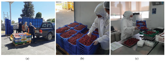
Figure 1.
Harvested fresh fruit that enters the industry’s selection and quality control process. (a) Fruit reception. All harvested fresh fruit is received for the quality control process. (b) Fruit selection. Harvested fresh fruit is visually checked before choosing a random sample to be inspected. (c) Fruit sample. One kilogram of red raspberries is selected as a sample unit from an entire batch.
It is important to note that the processing companies control the quality control process completely, which in some cases translates into bad practices, such as an underestimation of the quality of the fruit. This causes three problems. The first is regarding visual inspection, which is subjective and error-prone. The second is that only a few samples of the total number of trays are inspected, which usually does not reach statistical significance. This implies that based on the human expert’s criteria for the product, the quality, the purchase price, and the destination are determined. Finally, the industry wastes a lot of time and resources with the process of staff training for this task, because they are hired only during the fruit harvest, and they are not stable industry staff. Therefore, seeking clarity in the quality standards between the industry and the harvest by the farmer is one of the great challenges of the agro-industry. This work fits into this purpose. Note that the farmers do not classify the fruit, they cannot do it because this is a socioeconomic activity of family farming that uses a workforce unskilled for the recollection of the fruit. Thus, this responsibility is delegated to the industry, trusting in its criteria. The industry has a responsibility to determine a fair price by recognizing, identifying, and classifying the defects, errors, damage, and diseases of the fruit that enters the quality selection process. Likewise, the industry can analyze and judge the criteria that it has been using to classify this fruit and thus recognize the different biases between the industry and the harvest by the farmer. In short, when technology allows and detection algorithms are fully validated, fair, objective and unbiased quality ratings can be achieved. This is a challenge that begins with the use of this database. This database aims to solve one of the major problems in the industry. It will evaluate the largest amount of fruit as possible, and not a single sample as representing an entire batch. It is important to highlight that the RGB images in the database were acquired in an industrial context, just as is done, without process variations, see Figure 2a. The detection process in the machine takes between 2 and 5 min, see Figure 2b. This is an acceptable detection time for the industry.
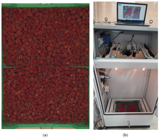
Figure 2.
Raspberries and equipment. (a) RGB image of raspberries in a tray to be evaluated. Note that it is a sample unit of the fruit, which is uniformly distributed throughout the tray, avoiding overlap between the fruit as much as possible. (b) Patented device for the acquisition of the images. Observe that the tray is placed at the bottom of the device, at the top is the lighting system, and an external computer to store the images.
Studies and investigations on the detection of the quality of the fruit are extensive and varied, specifically as regards raspberry fruit; to the best of our knowledge, this is the first RGB image database for the industrial applications of red raspberries’ automatic quality estimation. Table 1 shows some freely accessible database examples from different countries with the corresponding access to their repositories. Observe that the study objective focuses mainly on identifying and classifying diseases or defects to detect the quality of the fruit. This is because there is an interest in controlling the quality of the fruit since it can be significantly affected by damage or stains due to pathological injury, pests, or diseases, which ultimately degrade its quality and cause financial losses to the farmers.
It is well-known that data plays a critical role in machine learning approaches. The characteristics of these datasets must be clear and precise, such as their annotations or labels, because they directly influence the behavior of a model, which needs a training and testing stage to detect what has been learned, thus allowing applying the model to new data never seen before. Image quantity and resolution play a fundamental role during this process. In the examples in Table 1, the images are of high quality, with a very high resolution, which allows for the additional details that are stored in the pixels. These details are crucial in the analysis of the quality of the fruit, since, for example, a change in color, shade, or contrast, can help identify a disease or a defect; or to apply image techniques such as segmentation [3] or augmentation [4,5]. Please note that the images are generally captured in fieldwork, which is why it is often difficult to transport the necessary equipment to capture the appropriate images. In general, high-resolution cameras or cell phones are used. Furthermore, synthetic images can be generated from some samples. For example, in [6], a near-infrared (NIR) image generation method was used to yield a set of images re-processed from two public datasets with realistic results.
In this work, we present a free new database designed from a real industrial process with the aim of recognizing, identifying, and classifying the red raspberry’s quality from their RGB images in a tray, with recently harvested fresh fruit that enters the industry’s selection and quality control process, as Figure 1 shows. This major dataset has two large free packages: Images and Code, which allow researchers and students to improve red raspberry quality, by identifying different diseases and defects in the fruit and by overcoming limitations by increasing detection rate accuracy and reducing computation time. Second, we want to stimulate multidisciplinary research in diverse disciplines, such as agriculture, informatics, electronics, or data science, to develop practical applications in artificial intelligence, computer vision, or machine learning. A target of our free code, which is available with well-known methods to experiment with the data. Worth noting is that statistical-based learning methods have not been used before as image classifiers for fruit quality detection. In the first approach, four predictor learnings were used from descriptive statistical measures were used, such as the variance, the standard deviation, the mean, and the median. In the second approach, a statistical model based on the generalized extreme value distribution was estimated. This distribution has three parameters (location, scale, and shape) that can be used as predictor learnings from the raspberry tray image.
The two main contributions of this work are as follows:
- To the best of our knowledge, this is the first RGB image database for the industrial applications of red raspberries’ quality estimation in a tray. The images were acquired with a high-resolution camera in a controlled space, with a lighting system consisting of LED lights, which diffusely emit the illumination to avoid light hits (white spots) and shadows (black) on the fruit, as well as halogen lights. This allows excellent image characteristics to test image signal processing algorithms and ML approaches.
- To the best of our knowledge, the well-known statistical-based learning methods have not been used before as image classifiers for fruit quality detection. Statistical-based learning algorithms like this are extremely quick for use in real-time systems, but lack robustness.
This article is organized as follows: Section 2 introduces the standard quality of the red raspberries in the industry, and the diseases and defects used in this free database. Section 3 introduces the Raspberries-LITRP Database, and Section 4 the experiments applied to this dataset. Section 5 shows the results and discussion to apply this experimentation. Advantages, limitations, conclusions, and perspectives for future work are finally reported in Section 6.

Table 1.
Summary of some freely accessible databases related to studies on fruit quality. Data access can be consulted in the references.
Table 1.
Summary of some freely accessible databases related to studies on fruit quality. Data access can be consulted in the references.
| Fruits | Study Objetive | Image Dataset | Image Resolution | Code | Annotations | Repository | Country | Ref. |
|---|---|---|---|---|---|---|---|---|
| Raspberry | Diseases Defects | 286 | 3948 × 2748 | Yes | Yes | Raspberies LITRP | Chile | [This work] |
| Apple | Precision agriculture | 6089+ | Multifold | Not | Yes | Fuji Apples | España | Gene-Mola et al. [7,8] |
| Multifruit | Detection | 1515 | 3456 × 3456 | Not | Yes | QuinceSet | Japan | Kaufmane et al. [9] |
| Banana | Diseases Pathogens | 8000 | 3096 × 4128 | Not | Yes | PSFDMusa | India | Medhi et al. [10] |
| Guava | Disease | 527 | 2320 × 1540 | Not | Not | Guava | Bangladesh | Rajbongshi et al. [11] |
| Multifruit | Rotten detection | 12,335 | Multifold | Not | Not | Fresh Rotten | Bangladesh | Sultana et al. [12] |
| Multifruit | Detection | 127k synthetic images | Multifold | Not | Yes | deepNIR | Australia | Sa et al. [6] |
| Multifruit | Good, bad and mixed quality | 19,500 | 3024 × 3024 | Not | Not | FruitNet | India | Meshram et al. [13] |
| Palm date | Localization classification | 2576 | 5184 × 3456 4449 × 3071 4376 × 3375 | Not | Yes | Medjool Dates | Mexico | Perez-Perez et al. [14] |
| Apple | To augmentation methods | 800 | 1080 × 1920 | Not | Yes | Scifresh | USA | Gao et al. [5] |
| Grapes | Instance segmentation | 300 | 1365 × 2048 | Not | Yes | Embrapa WGISD | Brazil | Santos et al. [3] |
| Citrus | Diseases | 759 | 5202 × 3465 | Not | Yes | Citrus Plant | Pakistan | Harif et al. [15] |
| Multifruit | Robotic harvesting classification | 8079 | 5184 × 3456 4272 × 2848 | Not | Yes | Date Fruit | Saudi Arabia | Altaheri et al. [16] |
| Mango | Detection in tree canopy images | 1730 | 612 × 512 | Not | Yes | Mango YOLO | Australia | Koirala et al. [17] |
| Apple Mangoes Almonds | Multifold | 1120 1964 620 | 308 × 202 500 × 500 308 × 202 | Not | Yes | ACFR Orchard Fruit | Australia | Bargoti et al. [4] |
2. Red Raspberry
Raspberries contain a wide variety of vitamins, minerals, nutrients, sugars, and acids, which contribute to their sweetness, aroma, and healthful properties. The overall quality is when the fruit is harvested at optimum ripeness and at its highest sugar and aromatic level. The raspberry’s flavor should be sweet when ripe and not excessively acidic. The texture should be firm but juicy, and it should have a typical soft aroma. The nutritional benefits for human health are high due to the carbohydrate, vitamin, mineral, dietary fiber, and polyphenolic compounds that are present in the fruit. However, nevertheless, the composition of these chemicals can be highly variable depending on the environment, such as growing locations, fruit ripeness at harvest, and storage conditions.
2.1. Standard Quality Requirements for Raspberries in the Industry
Standard quality control is essential for every aspect of raspberry production. Its objective is to prevent a non-conforming product from reaching the next stage of the process or reaching the final customer. Therefore, different types of quality control are necessary, from the reception of the fruit to the final test of the finished product, along with its shelf life. In the first instance, the farmer is responsible for observing the fruit quality. The fruit that is susceptible to a slight deterioration due to its development and its tendency to perish, or that has a slight lack of freshness and turgidity, should be discarded. Obviously, they cannot be offered for sale or marketed. This is the first test to know if the conservation or the harvest criterion of the fruit should be changed. The raspberries in the industry must have some minimum and maturity requirements to enable them to withstand transportation, handling, and finally, to arrive in satisfactory condition at the place of destination. According to the International Codex Alimentarious [1], 300 grams of drained berry ingredients are used as a sample unit from an entire batch to segregate and assess raspberry quality. In Chile, each industry has its own standard based on this codex. On average, they evaluate 1 kilogram as a sample unit. The quality factors of raspberries are divided into two large groups:
Quick frozen:
- of good, reasonably uniform color, characteristic of the variety.
- clean, sound and practically free from foreign matter.
- free from foreign flavor and odor.
Visual defects:
- practically free from sand and grit.
- when presented as free-flowing, practically free from berries adhering one to another, and which cannot be easily separated when in the frozen state.
- reasonably free from uncolored berries.
- practically free from completely uncolored berries.
- reasonably free from stalks (cap stems).
- practically free from extraneous vegetable matter.
- reasonably free from damage or blemish due to pathological injury or pests (diseases).
- normally developed.
- of similar varietal characteristics.
- reasonably free from disintegrated berries or berries not intact.
2.2. Red Raspberry Diseases
Insects transmit viruses and are generally correlated to the local climate, thus they can cause damage to roots, canes, and fruit. Diseases, such as bacteria, fungi, and those caused by viruses, vary greatly between raspberry species and depend on soil types, such as clay versus sand. In another way, excessive or deficient levels of plant nutrients together with high temperatures, chemical toxicity hail, or wind, can affect the disease levels. We now introduce the two diseases studied in this paper, which are part of the database.
Albinism: It is a mottled white and is insipid and tasteless in flavor. In the course of the production season, the raspberries can acquire albinism during periods of warm weather followed by overcast and foggy skies or by an excess of nitrogen fertility. Once there is a change in the weather or throttling down on the quantity of nitrogen, albino fruit disappears. See Figure 3a.
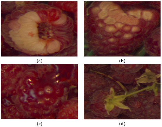
Figure 3.
Raspberries’ diseases and defects used in this database. (a) Albinism. (b) Fungus-Rust. (c) Over-ripeness. (d) Peduncle. Note that to the inexpert eye, the albinism disease can be confused with the over-ripeness defect.
Fungus-Rust: Rust is a disease of the foliage of raspberries, caused by the fungus Phragmidium rubi-idaei. Depending on the time of year, particularly during the wet weather, this fungus can produce several different types of spores, thus it changes the raspberry’s appearance. See Figure 3b.
2.3. Red Raspberry Defects
The defects admitted in a small percentage are the fruit bitten by birds or eaten by beetles, larvae, or worms.
Over-ripeness: It is given by softening of the fruit, in this state the loss of firmness is high, and its color change gives a dehydrated appearance. Its main characteristic is the coating color that turns to a darker red. See Figure 3c.
Peduncle: Is the point of attachment or stem attached to the fruit, or flower. See Figure 3d.
We refer the reader to [18,19,20] for a comprehensive treatment of raspberry fruit.
3. Raspberries-LITRP Database
In this section, we explain the process of red raspberry RGB image acquisition in Section 3.1, and image labeling in Section 3.2. Then, we introduce the database structure contents in Section 3.3 so that it can be used for free.
3.1. RGB Images Acquisition
The idea behind machine vision methods is basically to mimic the recognition and analysis process that occurs within the human brain. The objective of this acquisition was to obtain the best RGB image quality of raspberries using a controlled environment especially designed to be used in a typical fruit categorization routine within the industry. For this purpose, a device was designed, which is patented, to acquire RGB images of red raspberries in a tray and subsequently detect their quality through various algorithms. An RGB camera in the visible spectrum was used for the raspberry tray’s image acquisition. A Basler model acA4024-8gc GigE with a SONY IMX-304 CMOS color sensor of a maximum resolution of pixels with a pixel size of 3.45 mm was used. Figure 2a shows an example of the RGB image acquisition of red raspberries in a tray. In total, 286 raspberry tray images were acquired, each one with a resolution of pixels.
3.2. Image Labeling
The database has four classes, two for diseases such as albinism and fungus rust; and two for defects such as over-ripeness and peduncle. During the industrial-quality process, a human expert manually tagged each class for each tray of red raspberries, and an image was taken simultaneously. This process is crucial because we have the human expert’s annotations that are the data’s ground truth to permit a better performance in the training and testing stages during the classification and detection phases. The importance of these labeled images is that instead of processing the whole image, the detection algorithm focuses on specific Regions of Interest (RoI): diseases, or defects. For this purpose, for each tray image of red raspberries, the detection algorithm will seek RoIs using the results of previously processed bounding boxes (frames). Note that these bounding boxes were validated with the annotations of the human expert of the industry, see Figure 4. Then, for each tray image of red raspberries, a bounding box was fitted to each raspberry disease or defect class as follows, albinism 786 labels, fungus rust 164 labels, over-ripeness 115 labels, and peduncle 244 labels.
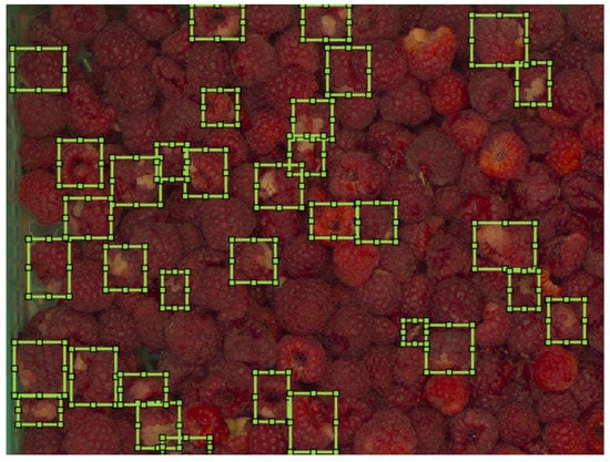
Figure 4.
Raspberry images labeled example. Due to the problem to resolve being to detect red raspberry quality, the goal is to precisely locate each raspberry in a tray image using a bounding box and label it with the relevant class, disease, or defect. Note that these bounding boxes vary greatly in size and can be located in any region of a tray image. Therefore, the first task is to generate a large set of ground truth bounding boxes to design a correct classifier to detect raspberry quality.
3.3. Raspberries-LITRP Database Structure
The Raspberries-LITRP database contains several folders with different images, such as raw original images of the raspberry trays, and the labeled images with the annotated diseases and defects previously preprocessed using bounding boxes through the MATLAB Image Labeler app, see Figure 4. Additionally, the MATLAB code is available to apply three approaches such as descriptive statistics, statistical modeling, and convolutional neural networks. This database is available in the repository from the LITRP laboratory within the Universidad Católica del Maule. To request a copy of the database, the researcher must fill out and sign the License Agreement Form, and then send it by email to the Principal Researcher. After receiving the email including the signed agreement document, a link will be sent to download the database.
The contents of the database are summarized below:
RGB images package
-

- A folder named OriginalTray with 286 raw original images of the raspberry trays, each one with a resolution of pixels.
-

- A folder named ProcessedTray with 1100 images of each raspberry tray splitting in four. Each image was split into four equal sections and resizing each of these with a resolution of pixels. This process was carried out with the aim of facilitating memory management during the training stage; please note that the quality of the image is maintained.
-

- A folder named AlbinismLabel with the next content:
-

- A folder named images with 786 albinism labels.
-

- A .mat file named AlbinismgTruth with the ground-truth information about the albinism disease class.
-

- A .mat file named imageLabelingSession from the albinism session created by the MATLAB Image Labeler app.
-
-

- A folder named FungusRustLabel with the next content:
-

- A folder named images with 164 fungus rust labels.
-

- A .mat file named FungusRustgTruth with the ground-truth information about the fungus rust disease class.
-

- A .mat file named imageLabelingSession from the fungus rust session created by the MATLAB Image Labeler app.
-
-

- A folder named OverripenessLabel with the next content:
-

- A folder named images with 115 over-ripeness labels.
-

- A .mat file named OverripenessgTruth with the ground-truth information about the over-ripeness defect class.
-

- A .mat file named imageLabelingSession from the over-ripeness session created by the MATLAB Image Labeler app.
-
-

- A folder named PenducleLabel with the next content:
-

- A folder named images with 244 peduncle labels.
-

- A .mat file named PenduclegTruth with the ground-truth information about the peduncle defect class.
-

- A .mat file named imageLabelingSession from the peduncle session created by the MATLAB Image Labeler app.
-
MATLAB code package
-

- A folder name code, with the following MATLAB scripts:
-

- main: This script is the main file that call all the subroutines: (a) load all ground-truth raspberry data, (b) split the data in into an 90% for training data and a 10% for testing data, and (c) call the classification experimental methods using statistical analysis and CNNs.
-

- statisticalAnalysis: to extract the features in a table for both training and testing stages using descriptive statistics and statistical modeling.
-

- cnnDetector: to estimate the raspberry quality in both training and testing stages, using CNNs approaches.
-
-

- A folder name mats, with the following .mat files:
-

- Tables for descriptive statistical testing and training stages.
-

- Tables for statistical modeling for testing and training stages.
-
-

- A folder named papers with our works on the subject in .pdf format.
-

- Disease and Defect Detection System for Raspberries Based on Convolutional Neural Network [2].
-

- A Review of Convolutional Neural Network Applied to Fruit Image Processing [21].
-

- Raspberries-LITRP Database: RGB images database for the industrial applications of red raspberries automatic quality estimation [our present work].
-
4. How to Experiment with the Database
In this section, we presented three well-known experimentation methodologies. The first method in Section 4.1 uses descriptive statistics measurements such as the variance, the standard deviation, the mean, and the median. In the second method, in Section 4.2, a statistical model was designed across the generalized extreme value distribution in Section 4.2. Please note that these two methods are designed to extract manual features from the data in Section 4.3, thus the chi-squared test was used to estimate the more significant features in Section 4.4. Finally, these features are used as inputs in a bilayer neural network in Section 4.5 that is used as a classifier to detect the fruit quality. The last method uses a CNN approach described in Section 4.6 of our previous work [2]. Finally, in Section 4.7 the performance metrics are introduced.
4.1. Descriptive Statistics
A preliminary analysis based on descriptive statistics is important because it gives the possibility to characterize the data based on its statistical properties. In other words, it allows us to obtain an idea of what the data are like. These properties can be summarized in four measures:
- Frequency distribution: It can be used to estimate how often something occurs, such as count, percentage, or frequency.
- Central tendency: It locates the distribution by various points, such as the mean, median, or mode.
- Variation or dispersion: It shows how the data are dispersed or spread, typically in relation to one of the measures from the central tendency; such as range, mean deviation, variance, or standard deviation.
- Location: It is standardized scores that describe how these scores fall in relation to one another, such as percentile ranks and quartile ranks.
4.2. Statistical Modeling
A statistical model is a probability distribution constructed to allow inferences to be drawn or decisions made from data. A probability distribution is a mathematical function that gives the probabilities of the occurrence of different possible outcomes to understand a specific process that explains or predicts future results. Typically, in many statistical applications, the interest in the process under study focuses on estimating some characteristics of the central tendency of the population, such as the mean, median, and mode. However, in some other application areas, the interest is in estimating the maximum or the minimum values, when the data have extreme conditions or singular values more than regular or mean values. The generalized extreme value distribution [22] is a flexible distribution that can be used for this purpose. Please note that generalized order statistics permit the unification of several models in one, via a distributional approach with unknown parameters.
Generalized Extreme Value Distribution
The generalized extreme value is a family that combines three different class types of distributions according to their tails, that correspond to the limiting distribution of block maxima. The types are:
- Type I (Gumbel domain): Distributions whose tails decrease exponentially.
- Type II (Fréchet domain): Distributions whose tails decrease as a polynomial.
- Type III (Weibull domain): Distributions whose tails are finite.
The generalized extreme value distribution has three parameters, called scale (), shape (), and location (), and its probability density function (PDF) is given by
where
determines the domain of the PDF as follows:
The parameters and can be calculated using the maximum likelihood estimators
The generalized extreme value distribution has the following advantages: (1) It can be adapted to the types of non-homogeneous patterns of extreme value variation observed in the dataset. (2) It is easy to incorporate all relevant information into an inference, and (3) it is beneficial to quantify uncertainties in estimation. Second, this distribution has the following disadvantages: (1) the model is developed using asymptotic arguments, which implies that necessary to take care is needed in treating them as exact results for finite samples. (2) The model is derived under an idealized circumstance, which may be reasonable, not exact, or only for a process under study. (3) The model may lead to wastage of information when implemented in practice because in the worst case, it can store only the maximum observed value over a specified period [23].
4.3. Feature Construction
The feature construction process is crucial for the design of a model and, consequently, the success of a machine-learning application. A model may use some or all of the estimated features to learn from the data. A ranking test, such as the Chi-square, can help make that decision, with the aim that the features may interact with each other to improve the model target. Please note that in a classification scheme, features may be differently correlated depending on the different classes. For example, for disease or defect classes, a model that uses descriptive statistics might use various features such as variance (), standard deviation (), mean (), and median (). On the other hand, a statistical model that uses the generalized extreme value can have characteristics according to its parameters, such as scale (), shape (), and location (). The features are also called attributes, predictor variables, explanatory variables, or independent variables [24]; and have their corresponding domain. Observe that Equation (7) shows the predictors for the descriptive statistical domain, and Equation (8) shows the predictors for its statistical model domain.
4.4. Feature Ranking
An important defining characteristic of a learning system is its use of features or rules as a fundamental building block of modeling [25]. Please note that the features or rules are defined from statistical parameters calculated from the data. Basically, a feature or rule defines a condition or a specific state to decide a class or take an action. The features can be used to generalize relationships between characteristics in the data and the target class to be classified or detected. Therefore, a feature ranking is interesting for discovering the most useful parameters and to design strategies to solve the model. The final model solution is a collaborative and competitive ensemble of classifiers or detectors, which captures generalized relationships between specific feature values in each condition designed and specific outcomes in the action or class. For this purpose, the Chi-square test can be used. The goal of this test is to examine whether each predictor variable is independent of a response variable using an individual chi-square test, and then rank the features according to their level of importance features according to their level of significance.
Chi-Square Test
The chi-square test is defined as
where represents the number of trials resulting in outcome i and represents the number of trials we would expect to result in outcome i when the hypothesized probabilities represent the actual probabilities assigned to each outcome.
It is important to note that if a boxplot or normal probability plot from data shows a substantial skewness or a substantial number of outliers, the chi-square-based inference procedures should not be applied. We refer the reader to [26,27] for a comprehensive treatment of the mathematical properties of the chi-square test.
4.5. Bilayer Neural Network
The ANN aims to associate a given input feature that represents the pattern to one of the classes of interest. The simplest ANN can be represented by the model given in Figure 5. The inputs are signals, samples, or features of the data. They are usually normalized to improve the learning algorithm. The weights are values used to weigh each one of the inputs. Their objective is the quantification of their relevance within neuron functionality. The bias (b) is a variable used to specify an appropriate threshold, in other words, it is the way to generate a trigger value toward the neuron output by the linear aggregator. The linear aggregator () assembles all input signals weighted by the weights to produce an activation of the neuron. The activate function (f) limits the neuron output within a reasonable range of values given by the difference () between the linear aggregator and the activation threshold. An excitatory potential for a positive value or inhibitory otherwise. The activation functions can be classified into two groups: (1) partially differentiable functions such as step function, signal function, and a symmetric ramp function. (2) fully differentiable functions such as logistic function, hyperbolic tangent function, and Gaussian function. The outputs are the final values produced by the neuron for a particular set of input signals. The model for one output y can be expressed as
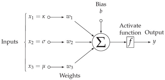
Figure 5.
Structure of a classical artificial neural network. The model shows how each neuron in a network can be implemented. This example is for data from three input features.
A Rectified Linear Unit (ReLU) layer can be used to perform the threshold operation on each element of the input, where any value less than zero is set to zero as follows
A bilayered neural network is a network with two hidden layers, see Figure 6. Each layer extracts patterns associated with the process of interest, where their learning algorithms architectures are based on the backpropagation algorithm and the competitive rules. During this process is when the network extracts discriminant characteristics from the input layer to make the feature map. Moreover, in the training stage, the forward (when the input is inserted into the network) and backward (when the weights are tuned) stages let the weights and thresholds of the neurons be adjusted automatically in each iteration, to reduce the final error between the network responses and the desired responses. For example, for a binary detection pattern, the first output may be for a healthy pattern, and the second output for a defective pattern.
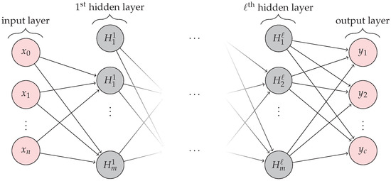
Figure 6.
A Topological configuration of a bilayer neural network used only two hidden layers . The input is propagated layer-by-layer toward the output layer, note that the outputs of the neurons from the first neural layer are the inputs of the neurons from the second hidden neural layer. This example is a multilayer-perceptron for input features data, layers, and outputs.
To use the bilayered neural network as a quality detector, the observations are classifiers according to their scores using the softmax activation function. These scores, which accompany the end fully connected layer in the network, are estimated through the decision rule or posterior probability, that an observation x is of class k
where is the conditional probability of x given the class k, K is the number of classes in the response variable, is the prior probability for class k, it tells us how likely each of the classes is a prior, or before the data x is observed, and is the k output from the end fully connected layer for the observation x. We refer the reader to [28,29] for a comprehensive treatment of the mathematical properties of the neural networks.
4.6. Convolutional Neural Network
The convolutional neural network also called ConvNet or simply CCN is a special kind of multilayer ANN whose original architecture, called LeNet-5, was first proposed by LeCun et al. in [30]. CNNs were inspired by the behavior of how neurons in the visual brain cortex fired each other (activation function) to respond to different input stimuli such as an image (features). Therefore, a certain group of neurons comes together focusing on particular properties to carry out a specific task. This is the idea behind the CCNs and their direct relation with the CVS. The underlying idea of CVS is to describe the world that we see in one or more images, and reconstruct their properties, such as shape, lighting, or color distributions, in the most similar way possible to how our brain would do it, in our case, mimic the process of the quality fruit recognition analysis that carries out by the industry human expert. The idea is to detect natural objects in heterogeneous samples with high variability between their classes, such as the quality and diseases of raspberries. To achieve this, different artificial neural network (ANN) architectures are widely used. ANNs are computational models inspired by the behavior nervous system of living beings. This implies that they can be interconnected with other neurons, with the objective of learning and saving information to make decisions or adapt to new data. Similar to how biological neurons work it. Convolutional neural networks (CNN) are specialized ANNs designed to process different types of data using convolution mathematical operation. They have a known grid-like topology that can be used in time series data (1-D grid) or image data (2-D grid), that take samples at regular time intervals, or across pixels, respectively. For a recent comprehensive review of CNNs applied to fruit image processing, see [21,31,32,33].
As an illustration, consider Figure 7. The input image enters into the CNN, which is composed of stacks of convolutional and pooling layer pairs. For the feature map extraction, the convolution layers convert the image using the convolution operation, similar to applying several digital filters. On the other hand, the pooling layer combines the neighboring pixels into a single pixel. Therefore, CNN extracts its own parameters directly from the image as a set of arrays called feature maps, these maps are composed of four main components: a filter bank called kernels, a convolution layer, a non-linearity activation function, and a pooling or subsampling layer. Note that this process is a dimensional reduction of the image. During the training stage, the weights of both layers are estimated. The feature map extraction is computed, and the input is classified based on this feature map. We refer the reader to [2,31,34] for a comprehensive explanation of CNNs. Regions with convolutional neural networks (R-CNN) are used to find and classify diseases and defects in raspberries, called objects, in a raspberry tray image in the industry. The process combines rectangular region proposals (images labeled) with convolutional neural network features in a two-stage detection algorithm. The first stage identifies a subset of regions in an image that might contain a disease or defect (object) to be classified in the second stage, see Figure 7. Transfer learning from a network trained from a large collection of images is used for this purpose. In this way, the Faster R-CNN detector only processes those regions that are likely to contain the disease or defect (object). This reduces the high computational cost, and it permits to obtain of model parameters from the labeled data. The network maps the input data to a specific class label. Thus, the pretrained network has already learned a rich set of raspberry fruit image features that are applicable to a wide range of new raspberry tray images. A starting point to solve a new classification or detection of fruit quality. This is why the training stage is crucial to correctly detect the class labels for new instances, which is typically done during the testing stage. Exist different architectures for this proposal such as LeNet, AlexNet, ZFNet, VGGNet, GoogLeNet, ResNet, Inception, Xception, SqueezeNet, and SuffleNet, and the list continues to evolve.
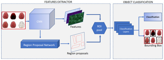
Figure 7.
Object detection using the Faster R-CNN process. The ROI pool consists of the features and the proposal regions to be classified in the next stage.
4.7. Performance Metrics
Let a binary classifier mapping in for the classes , where is the positive class, and is the negative class, and is the instance space, a set of all possibles instances. For a test dataset we have the following definitions:
Number of Positives
Number of Negatives
Number of True Positives
Number of False Positives
Number of True Negatives
Number of False Negatives
Recall or True Positive Rate or Sensitivity or Hit Rate
Is the proportion of positives correctly classified, or the estimation of , it is defined as
False Positive Rate or False Alarm Rate
Is the number of misclassified positive or false negative, or the estimation of , it is defined as
Accuracy
Is the probability of an arbitrary class being classified correctly, or the estimation of , it is defined as
4.8. Methodology Summary
Let be he matrix corresponding to an image of the raspberry tray to be analyzed, and ,and the sets of preprocessing images labeled with two diseases and two defects: albinism, fungal rust, over-ripeness, and peduncle, respectively. Figure 8, Figure 9 and Figure 10 show the different methodologies proposed in this paper:
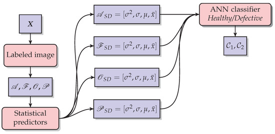
Figure 8.
The methodology used in descriptive statistics for each disease and defect. Statistical predictors such as variance (), standard deviation (), mean (), and median () are the inputs to be classified using a neural network. The Output is the class raspberry healthy () or the class raspberry defective ().
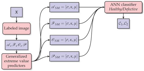
Figure 9.
The methodology used in statistical modeling for each disease and defect. Generalized extreme value parameters are the statistical predictors such as scale (), shape (), and location (). They are the inputs to be classified using a neural network. The output is the class raspberry healthy () or the class raspberry defective ().
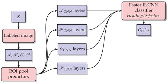
Figure 10.
The methodology used in the Faster R-CNN modeling for each disease and defect. The Faster R-CNN approach extracts its own parameters directly from the image as a set of arrays called feature maps, these maps are composed of four main components: a filter bank called kernels, a convolution layer, a non-linearity activation function, and a pooling or subsampling layer. Second, the proposed regions of the network are estimated. The feature maps and the region proposal together are the ROI pool predictors, which are used to classify and detect fruit quality for each layer. The Output is the class raspberry healthy () or the class raspberry defective ().
5. Results and Discussion
In this work, we presented a new database of red raspberries in a tray using RGB images to detect their quality in industrial applications. This database was evaluated using three well-known methods in order to estimate its classification performance, with promising results that can be implemented in real-time systems. Two statistical-based learning methods are coupled with a classical ANN, and the other one uses a Faster R-CNN method. As a first instance, the classification is based on a binary learning system between a healthy raspberry vs. a raspberry with a disease or defect. Please note that the defective raspberries were labeled previously using a bounding box as follows: 786 albinism disease labels, 164 fungus rust disease labels, 115 over-ripeness defect labels, and 244 peduncle defect labels. This section shows the results and discussion when applying the experimentation from Section 4 using 90% for the training set, and 10% for testing.
For the statistical-based learning methods, the bounds found are very interesting. For descriptive statistics, the bounds based on the median and variance allow us to differentiate between the diseases studied, while the thresholds based on the defects are not very clear. This may be because their bound values share part of the healthy raspberry values of the fruit. Similar results occur with statistical modeling using the generalized extreme value distribution. In general, all the parameters based on their bounds for a binary learning system allow differentiating between a healthy raspberry vs. a raspberry with disease or defect. Except for the shape () parameter for the peduncle, and the scale () parameter for the two defects. These results can be corroborated in the predictor ranking from Section 5.3. It is important to emphasize that the feature ranking test can vary between the different classes. This suggests that in the case of using the two most representative features as predictors, they must be different between classes. These results are in tune with the results of our previous work [2]. In this work, we found that different network architectures can be used to detect different raspberry diseases or defects. Another topic of interest in using statistical methods is the importance of bounds for the features. Because identifying the learning boundaries helps to ensure the success of model learning, by having a coverage limit, then it is possible to guarantee both the proper initialization of the population and the maintenance of the necessary learning time to yield the necessary outcomes. A big plus of CNNs is that they learn directly from data, eliminating the need for manual feature extraction, with highly accurate results during the classification and detection stages.
5.1. Descriptive Statistics
In this section, descriptive statistical measures were used as predictors, such as the variance, the standard deviation, the mean, and the median, see Equation (7). Table 2 shows that diseases and defects can be easily discriminated against according to their average threshold value and bounds. Remember that the classification is based on a binary learning system between a healthy raspberry vs. a defective raspberry, as shown in Figure 8.
Table 2.
Analysis using descriptive statistics. The table shows the average thresholds and the learning bounds of each class.
Table 2 shows that the average threshold for a healthy raspberry is lower for all predictors, except for the standard deviation for the over-ripeness defect. While for the bounds, comparisons can be made even though there are some overlaps. Let us take the median predictor as an example. The median has an average threshold value of for a healthy raspberry, which is lower than the rest of the average threshold values: for albinism disease, for fungus rust disease, for over-ripeness defect, and for peduncle defect. This suggests that each disease and each defect of a raspberry concerning a healthy raspberry can be discriminated by an average threshold. Similarly, it happens with the bounds. A healthy raspberry is between the values of . Then the lower bound has a value of 56 and the upper bound has a value of 169. By comparing the lower bounds, we can observe that the 56 value is different for all predictors. A value for albinism disease, a 27 value for fungus rust disease, a 59 value for over-ripeness defect, and a value for peduncle defect. While for the upper bounds, we can observe that the value of 169 is lower for all descriptors. A value for albinism disease, a 233 value for fungus rust disease, a 203 value for over-ripeness defect, and a 241 value for peduncle defect. There is some overlap. In the same way, it happens with the other predictors. Applying this analysis of all the predictors together, we suggest that these differences between the lower and upper bounds can achieve good performance on the ML approach. Note that these predictors are the input for the neural network to classify and detect diseases and defects in raspberries, see Figure 8. Figure 11 shows the representation of the distribution of numerical data for each class studied. Observe the large similarity that all the figures have.
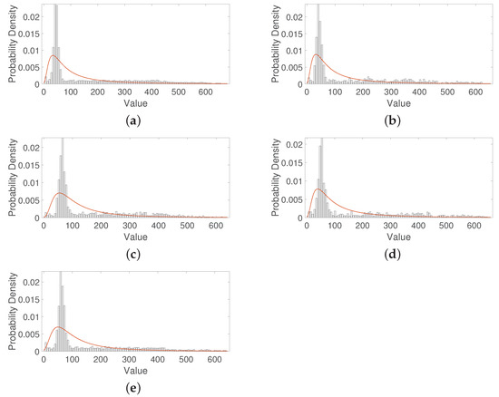
Figure 11.
Histograms and generalized extreme value fitting from the raspberry diseases and defects used in this database. (a) Raspberries with albinism disease. (b) Raspberries with the fungus rust disease. (c) Raspberries with the over-ripeness defect. (d) Raspberries with peduncle defect. (e) Healthy raspberry.
5.2. Statistical Modeling
This section shows the results to when applying Equations (1)–(3) related to the generalized extreme value distribution. Figure 11 shows the different histograms for each class. Please note how the distribution across the frequency of the numerical data is very similar and difficult to differentiate. One solution to this is to use statistical modeling through some probability distribution. Therefore, from the raspberry trays’ images, the generalized extreme value distribution was estimated for each class, see the red line in Figure 11. Table 3 shows the three parameters resulting from applying this distribution. For a binary learning system such as healthy raspberry vs. defective raspberry, see Figure 9; all average thresholds can be used for this discrimination, despite the fact that they are very close to each other. With respect to the bounds, the location parameter () and the shape () parameter can be interesting predictors to detect and discriminate the different, see Equation (8). While the scale () parameter values are very close between them and thus difficult to differentiate it.
Table 3.
Analysis using the generalized extreme value distribution. The table shows the average thresholds and the learning bounds of each class.
Let us take the location parameter predictor () as an example. has an average threshold value of for a healthy raspberry, which is different with respect to the rest of the average threshold values, for albinism disease, for fungus rust disease, for over-ripeness defect, and for peduncle defect. This suggests that each disease and each defect of a raspberry with respect to a healthy raspberry can be discriminated by an average threshold. Similarly, it happens with the bounds. A healthy raspberry is between the values , which is different too, with respect to the rest bounds values, for albinism disease, for fungus rust disease, for over-ripeness defect and for peduncle defect. Note that all values of the lower and upper bounds are different from each other, except for a small overlap between the upper bounds of the diseases. Similarly, there is an overlap between the other predictors. Applying this analysis of all the predictors together, we suggest that these differences between the lower and upper bounds can achieve good performance on the ML approach. Please note that these predictors are the input for the neural network to classify and detect diseases and defects in raspberries, as shown in Figure 9.
5.3. Feature ranking test
Boxplots were estimated from data, with the aim of verifying both the asymmetric and the outlier values. Figure 12 shows that the boxplots from the data are very symmetric. The outliers are not representing a problem because they are an outcome of the variability from data acquisition as seen in the variance of Table 2. Therefore, the chi-square test used to determine feature ranking can be applied using Equation (9).
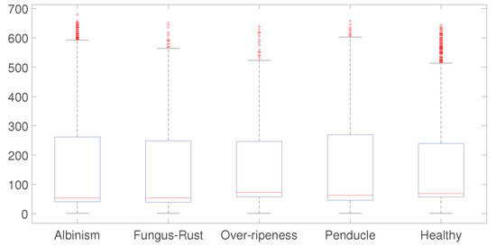
Figure 12.
Boxplots of each class show a generalized symmetry, and no significant outliers.
Figure 13 shows the feature ranking tests, using descriptive statistics with its predictors such as variance, standard deviation, mean, and median; and Figure 14 shows the feature ranking tests using statistical modeling, across the generalized extreme value distribution, respectively, across its predictors such as shape, scale, and location. Please observe these interesting results that can be corroborated with Table 2 and Table 3. Figure 13 shows that the median has a significant rank for all the diseases and defects studied and therefore can be used as a strong feature, while Figure 14 shows that the parameter, related to the location, and the parameter, related to the shape, are strong features. Please note the interesting central tendency and location in both figures. These features are determinants for the learning stages of classification and detection.
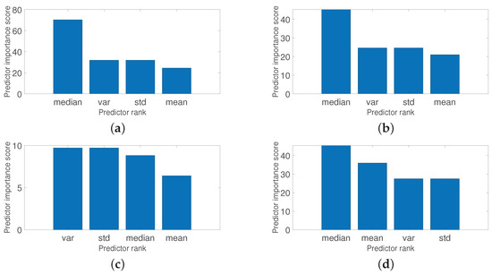
Figure 13.
Feature ranking from the raspberries diseases and defects using descriptive statistics. (a) Albinism. (b) Fungus-Rust. (c) Over-ripeness. (d) Peduncle.
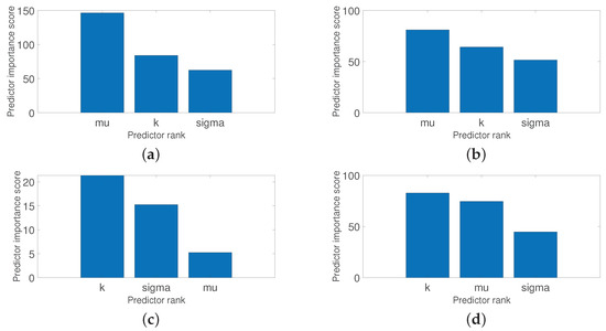
Figure 14.
Feature ranking from the raspberries diseases and defects using statistical modeling. (a) Albinism. (b) Fungus-Rust. (c) Over-ripeness. (d) Peduncle.
5.4. Classification Performance
In this section, classification performance results using the three well-known methodologies are exposed, see Figure 8, Figure 9 and Figure 10. Table 4 shows the classification performance metric under 100 iterations of these three methodologies studied, namely recall, false positive rate, and accuracy through Equations (20)–(22), respectively. Please note that this classification performance metric is directly related to the Receiver operating characteristic (ROC) curve, which is an output performance of the learning system. Remember that the database has 786 albinism disease labels, 164 fungus rust disease labels, 115 over-ripeness defect labels, and 244 peduncle defect labels.
Table 4.
True positive rate or recall (TPR), false positive rate (FPS), and accuracy (ACC) classification performance metric for the three methodologies used, such as a descriptive statistical coupled with an ANN (DS+ANN), statistical modeling coupled with an ANN (SM+ANN), and Faster R-CNN.
These results are very interesting. Please note that all the classifiers have difficulty in detecting the over-ripeness defect, this can be due to two reasons. The first is because the color of the raspberry is preserved, but darker, and the second is the over-ripeness is the defect with the least number of labels. Faster R-CNN is the best methodology with respect to the statistical-based learning methods coupled with an ANN. However, they also perform very well for all the defective raspberries studied. Faster R-CNN is very sensitive (TPR) with high fall-out response (FPR), which makes it have excellent detection accuracy. Second, the statistical-based learning methods are very sensitive (TPR) too, but with low fall-out response (FPR), nevertheless, they have good accuracy. This suggests that they may need a regularization parameter to help tune the FPR. Faster R-CNN detects fungus rust disease fairly well, even though the number of tags is low, while albinism disease and peduncle defect achieved a high detection performance, 98% and 100%, respectively. This is consistent with the results of our previous work [2]. The performance detection using the statistical-based models coupled with an ANN are very similar, they are all around 80%, except for the over-ripeness defect. For an illustration, Table 5 shows some recent works on fruit-based quality detection. CNN-based methods are currently at the forefront of developments to detect diseases or defects in different fruit. However, there are still works with other types of techniques, without using neural networks, for example, in [35] the classification was estimated directly using the segmentation technique in olives yielding a reasonable detection rate. Note that the detection accuracy rate is high in all studies, suggesting that there is a concern to improve the quality detection of diverse fruit in agribusiness.
Table 5.
Summary of some works related to studies on fruit-based quality detection. Note that CNNs predominate in DL approaches.
Because Table 5 shows different studies, with different techniques, for different fruit, with different amounts of images in their datasets, a comparative analysis should be made regarding fruit-based quality detection. Remarkable that CNN-based methods are currently at the forefront of developments in fruit quality detection. These methods generally outperform conventional feature-based extraction methods, but the computational cost can be sufficiently high. Therefore, feature-based extraction methods must not be detracted from them. They continue to prove themselves invaluable in several applications. Furthermore, the computational cost is usually pretty low. The performance detection rate of this work regarding those exposed in Table 5 shows excellent results in the detection of the quality of the fruit, both for the statistical-based learning methods and for the Faster R-CNN. These results suggest that we are accomplishing the parameters and standards of the industry to discriminate between a healthy raspberry and a raspberry with a disease or defect. Finally, this work showed that fruit-based quality detection works are highly diverse.
6. Conclusions
This work presented a new database of red raspberries in a tray using RGB images to detect their quality in industrial applications, as shown in Table 1. The images were acquired with a high-resolution camera in an ambient controlled space, with a lighting system consisting of LED lights, which diffusely emit the illumination to avoid light hits (white spots) and shadows (black areas) on the fruit, as well as halogen lights. This allows excellent image characteristics to test image signal processing algorithms and ML approaches without a preprocessing stage. This database contains two typical diseases and two typical defects that can be in the recently harvested fresh fruit that enter the industry’s selection and quality control process. This database was evaluated using three well-known methods, as follows:
The first two are related to feature extraction from statistical-based learning methods coupled with a conventional ANN as a classifier and a detector. Please note that these methods have not been used before as image classifiers for fruit quality detection. For descriptive statistics, all predictors were used. However, the median and the variance were the most representative predictors to discriminate between a healthy raspberry and a raspberry with some disease or defect, as shown in Figure 13. The same occurs with statistical modeling based on the generalized distribution of extreme values. All predictors were used, but the shape and the location parameters were the most significant predictors, as shown in Figure 14. Remember that these predictors are the input of the ANN whose function is to classify the raspberry. The generalized extreme value distribution achieved an 84.50% detection rate on average, while the descriptive statistical method achieved an 81% detection rate on average in the raspberry quality detection. The last method uses directly Faster R-CNN as feature extraction, classifier, and detector, achieving a 91.2% detection rate on average. These results are shown in the first three rows of Table 5. Please note that they are within detection rate standards.
It is interesting to emphasize that the statistical-based learning methods are quite simple, but nevertheless, they can be a potential ally in decision-making regarding raspberry diseases and defects. These results show promising results, which can shed new light on fruit quality standards’ methodology in the industry.
6.1. Advantages
The main advantages are that the database is easy to use, and the user can work with or without feature extraction methods, as well as different architectures using CNNs. For a new class, the database can be retrained, but only for that class. The pretrained CCNs permit transfer learning, allowing a reduction of the number of images and time required for training. The network is fine-tuned by making small adjustments to the weights, so that the feature maps learned for the original training are slightly adjusted to support the new class. Furthermore, the user can try different preprocessing techniques before using a classification learning system. Finally, this methodology can be expanded to other fruit.
6.2. Limitations
The main limitation is related to the angle and rotation of the raspberry in a tray during image capture. Remember that a small random sample is selected to define a complete batch during the quality control process in the industry, see Figure 1. Although the expert in quality control of the industry distributes the fruit in the tray in the most orderly way possible, avoiding overlaps between them. It is too hard to be 100% sure with a single layer. The trays cannot be shaken, and the fruit cannot be turned manually because it is a very delicate fruit. This limitation must be resolved at some point.
The other limitation is related to the training time using CNNs. In the case of training the entire database, this can be time-consuming due to the numerous parameters within the layers. For example, the ResNet algorithm can take around two weeks to fully train from scratch, while traditional feature extraction algorithms take a few seconds to a few hours to train an algorithm.
6.3. Future Work
Perspectives for future works are to increase the database with new diseases and defects classes. We also plan to improve classification and detection methods, identify different diseases and defects in fruit and overcoming limitations, increase the performance detection rate accuracy and reduce computation time. We will work together with industry quality experts to improve data estimation, detailing similarities and errors to streamline the process and improve fruit quality grading and detection accuracy. In addition, we will incorporate image signal preprocessing stages such as image segmentation, perform a multispectral analysis of red raspberries to estimate their best wavelength band of them. Regularization parameter estimation for the statistical-based learning methods at the classification stage is necessary to improve detection. Finally, the methodology should be expanded to other types of fruit in the industry.
Author Contributions
A.Q.R.: methodology, software, validation, formal analysis, conceptualization, writing—original draft and resources; M.M.: funding acquisition, conceptualization, methodology and writing—review; J.N.-T.: software and resources; C.F.: funding acquisition; A.V.: funding acquisition. All authors have read and agreed to the published version of the manuscript.
Funding
This research was funded by Innovation Fund for Competitiveness-FIC, Government of Maule, Chile-Project Transfer Development Equipment Estimation Quality of Raspberry, code 40.001.110-0. (Esta investigación fue financiada por el Fondo de Innovación para la Competitividad- FIC, Gobierno de Maule, Chile-Proyecto de Transferencia de Desarrollo de Equipo de Estimación de Calidad de la Frambuesa, código 40.001.110-0).
Institutional Review Board Statement
Not applicable.
Informed Consent Statement
Not applicable.
Data Availability Statement
Not applicable.
Acknowledgments
The authors thank the Laboratory of Technological Research in Recognition of Patterns (www.litrp.cl, accessed on 7 November 2022) of the Universidad Catolica del Maule, Chile, for providing the computer servers where the experiments were carried out.
Conflicts of Interest
The authors declare no conflict of interest.
Sample Availability
The data used in this study is available upon direct request to Marco Mora (mmora@ucm.cl) head of the Laboratory of Technological Research in Recognition of Patterns (www.litrp.cl, accessed on 10 November 2022).
Abbreviations
The following abbreviations are used in this manuscript:
| ANN | Artificial Neural Network |
| AP | Average Precision |
| CNN | Convolutional Neural Network |
| Cvs. | computer vision systems |
| DB | database |
| DL | Deep Learning |
| DR | Detection Rate |
| FCNN | Fully Convolutional Network |
| IQF | Individually quick-frozen |
| ML | Machine Learning |
| RGB | Red-Green-Blue |
| RNN | Recurrent Neural Network |
| RoI | Regions of Interest |
References
- Codex Alimentarious. Standard for Quick Frozen Raspberries CXS 69-1981, Adopted in 1981. Amended in 2019. Available online: https://www.fao.org/fao-who-codexalimentarius/en/ (accessed on 10 November 2022).
- Naranjo-Torres, J.; Mora, M.; Fredes, C.; Valenzuela, A. Disease and Defect Detection System for Raspberries Based on Convolutional Neural Networks. Appl. Sci. 2021, 11, 11868. [Google Scholar]
- Santos, T.T.; de Souza, L.L.; dos Santos, A.A.; Avila, S. Grape detection, segmentation, and tracking using deep neural networks and three-dimensional association. Comput. Electron. Agric. 2020, 170, 105247. Available online: https://zenodo.org/record/3361736#%23.Y0SRk9LMLlg (accessed on 10 November 2022).
- Bargoti, S.; Underwood, J. Deep fruit detection in orchards. In Proceedings of the 2017 IEEE International Conference on Robotics and Automation (ICRA), Singapore, 29 May 2017–3 June 2017; pp. 3626–3633. Available online: http://data.acfr.usyd.edu.au/ag/treecrops/2016-multifruit/ (accessed on 10 November 2022).
- Gao, F.; Fu, L.; Zhang, X.; Majeed, Y.; Li, R.; Karkee, M.; Zhang, Q. Multi-class fruit-on-plant detection for apple in SNAP system using Faster R-CNN. Comput. Electron. Agric. 2020, 176, 105634. Available online: https://github.com/fu3lab/Scifresh-apple-RGB-images-with-multi-class-label (accessed on 10 November 2022). [CrossRef]
- Sa, I.; Lim, J.Y.; Ahn, H.S.; MacDonald, B. deepNIR: Datasets for Generating Synthetic NIR Images and Improved Fruit Detection System Using Deep Learning Techniques. Sensors 2022, 22, 4721. Available online: https://inkyusa.github.io/deepNIR_dataset/ (accessed on 10 November 2022). [PubMed]
- Gene-Mola, J.; Vilaplana, V.; Rosell-Polo, J.R.; Morros, J.R.; Ruiz-Hidalgo, J.; Gregorio, E. KFuji RGB-DS database: Fuji apple multi-modal images for fruit detection with color, depth and range-corrected IR data. Data Brief 2019, 25, 104289. [Google Scholar]
- Gene-Mola, J.; Sanz-Cortiella, R.; Rosell-Polo, J.R.; Morros, J.R.; Ruiz-Hidalgo, J.; Vilaplana, V.; Gregorio, E. Fuji-SfM dataset: A collection of annotated images and point clouds for Fuji apple detection and location using structure-from-motion photogrammetry. Data Brief 2020, 30, 105591. Available online: https://www.grap.udl.cat/en/publications/datasetsg (accessed on 10 November 2022). [CrossRef]
- Kaufmane, E.; Sudars, K.; Namatevs, I.; Kalnina, I.; Judvaitis, J.; Balass, R.; Strauti, S. QuinceSet: Dataset of annotated Japanese quince images for object detection. Data Brief 2022, 42, 108332. Available online: https://zenodo.org/record/6402251#%23.Y2ARltLMLlg (accessed on 10 November 2022).
- Medhi, E.; Deb, N. PSFD-Musa: A dataset of banana plant, stem, fruit, leaf, and disease. Data Brief 2022, 43, 108427. Available online: https://data.mendeley.com/datasets/4wyymrcpyz/1 (accessed on 10 November 2022).
- Rajbongshi, A.; Sazzad, S.; Shakil, R.; Akter, B.; Sara, U. A comprehensive guava leaves and fruits dataset for guava disease recognition. Data Brief 2022, 42, 108174. Available online: https://data.mendeley.com/datasets/x84p2g3k6z/1 (accessed on 10 November 2022).
- Sultana, N.; Jahan, M.; Uddin, M.S. An extensive dataset for successful recognition of fresh and rotten fruits. Data Brief 2022, 44, 108552. Available online: https://data.mendeley.com/datasets/bdd69gyhv8/1 (accessed on 10 November 2022). [CrossRef]
- Meshram, V.; Patil, K. FruitNet: Indian fruits image dataset with quality for machine learning applications. Data Brief 2022, 40, 107686. Available online: https://data.mendeley.com/datasets/b6fftwbr2v/1 (accessed on 10 November 2022). [CrossRef]
- Perez-Perez, D.B.; Salomon-Torres, R.; Garcia-Vazquez, J.P. Dataset for localization and classification of Medjool dates in digital images. Data Brief 2021, 36, 107116. Available online: https://data.mendeley.com/datasets/872xk9npmz/1 (accessed on 10 November 2022). [CrossRef]
- Rauf, H.T.; Saleem, B.A.; Lali, M.I.U.; Khan, M.A.; Sharif, M.; Bukhari, S.A.C. A citrus fruits and leaves dataset for detection and classification of citrus diseases through machine learning. Data Brief 2019, 26, 104340. Available online: https://data.mendeley.com/datasets/3f83gxmv57/2 (accessed on 10 November 2022). [CrossRef] [PubMed]
- Altaheri, H.; Alsulaiman, M.; Muhammad, G.; Amin, S.U.; Bencherif, M.; Mekhtiche, M. Date fruit dataset for intelligent harvesting. Data Brief 2019, 26, 104514. Available online: https://ieee-dataport.org/open-access/date-fruit-dataset-automated-harvesting-and-visual-yield-estimation (accessed on 10 November 2022). [PubMed]
- Koirala, A.; Walsh, K.; Wang, Z.; McCarthy, C. Deep learning for real-time fruit detection and orchard fruit load estimation: Benchmarking of ’mangoyolo’. Precis. Agric. 2019, 20, 1107–1135. Available online: https://figshare.com/articles/dataset/MangoYOLO_data_set/13450661 (accessed on 10 November 2022).
- Funt, R.C.; Hall, H.K. Raspberries; CABI: Wallingford, UK, 2013. [Google Scholar]
- Dodge, B.; Wilcox, R. Diseases of Raspberries and Blackberries; CreateSpace: Scotts Valley, CA, USA, 2017. [Google Scholar]
- U.S. Deptartment of Agriculture. Raspberries. How To Plant, Grow and Harvest Raspberries: USDA Bulletin; CreateSpace: Scotts Valley, CA, USA, 2017.
- Naranjo-Torres, J.; Mora, M.; Hernández-García, R.; Barrientos, R.J.; Fredes, C.; Valenzuela, A. A Review of Convolutional Neural Network Applied to Fruit Image Processing. Appl. Sci. 2020, 10, 3443. [Google Scholar]
- Kotz, S.; Nadarajah, S. Extreme Value Distributions: Theory and Applications; ICP: London, UK, 2001. [Google Scholar]
- Coles, S. An Introduction to Statistical Modeling of Extreme Values; Springer: Berlin/Heidelberg, Germany, 2001. [Google Scholar]
- Flach, P. Machine Learning. The Art and Science of Algorithms that Make Sense of Data; Cambridge University Press: Cambridge, UK, 2001. [Google Scholar]
- Guyon, I.; Elisseeff, A. An Introduction to Variable and Feature Selection. J. Mach. Learn. Res. 2003, 3, 1157–1182. [Google Scholar]
- Voinov, V.; Nikulin, M.S.; Balakrishnan, N. Chi-Squared Goodness of Fit Tests with Applications; Academic Press: Cambridge, MA, USA, 2013. [Google Scholar]
- Ott, R.L.; Longneckern, M.T. An Introduction to Statistical Methods and Data Analysis; Cengage Learning: Boston, MA, USA, 2015. [Google Scholar]
- da Silva, I.N.; Spatti, D.H.; Flauzino, R.A.; Liboni, L.H.B.; dos Reis Alves, S.F. Artificial Neural Networks, A Practical Course; Springer: Berlin/Heidelberg, Germany, 2017. [Google Scholar]
- Hagan, M.T.; Beale, M.H.; Demuth, H.B. Neural Network Design; Martin Hagan: Stillwater, OK, USA, 2022. [Google Scholar]
- LeCun, Y. Generalization and network design strategies. In Technical Report CRG-TR-89-4; University of Toronto: Toronto, ON, Canada, 1989. [Google Scholar]
- Mamat, N.; Othman, M.F.; Abdoulghafor, R.; Belhaouari, S.B.; Mamat, N.; Mohd Hussein, S.F. Advanced Technology in Agriculture Industry by Implementing Image Annotation Technique and Deep Learning Approach: A Review. Agriculture 2022, 12, 1033. [Google Scholar]
- Wang, C.; Liu, S.; Wang, Y.; Xiong, J.; Zhang, Z.; Zhao, B.; Luo, L.; Lin, G.; He, P. Application of Convolutional Neural Network-Based Detection Methods in Fresh Fruit Production: A Comprehensive Review. Front. Plant Sci. 2022, 13, 868745. [Google Scholar]
- Wang, X.A.; Tang, J.; Whitty, M. Data-centric analysis of on-tree fruit detection: Experiments with deep learning. Comput. Electron. Agric. 2022, 194, 106748. [Google Scholar] [CrossRef]
- Khan, S.; Rahmani, H.; Shah, S.A.A.; Bennamoun, M. A Guide to Convolutional Neural Networks for Computer Vision; Morgan and Claypool: San Rafael, CA, USA, 2018. [Google Scholar]
- Cano Marchal, P.; Satorres Martínez, S.; Gómez Ortega, J.; Gámez García, J. Automatic System for the Detection of Defects on Olive Fruits in an Oil Mill. Appl. Sci. 2021, 11, 8167. [Google Scholar] [CrossRef]
- Gao, J.; Dai, S.; Huang, J.; Xiao, X.; Liu, L.; Wang, L.; Sun, X.; Guo, Y.; Li, M. Kiwifruit Detection Method in Orchard via an Improved Light-Weight YOLOv4. Agronomy 2022, 12, 1–15. [Google Scholar] [CrossRef]
- Huang, H.; Huang, T.; Li, Z.; Lyu, S.; Hong, T. Design of Citrus Fruit Detection System Based on Mobile Platform and Edge Computer Device. Sensors 2022, 22, 1–14. [Google Scholar]
- Wang, N.; Qian, T.; Yang, J.; Li, L.; Zhang, Y.; Zheng, X.; Xu, Y.; Zhao, H.; Zhao, J. An Enhanced YOLOv5 Model for Greenhouse Cucumber Fruit Recognition Based on Color Space Features. Agriculture 2022, 12, 1556. [Google Scholar] [CrossRef]
- Momeny, M.; Jahanbakhshi, A.; Neshat, A.A.; Hadipour-Rokni, R.; Zhang, Y.D.; Ampatzidis, Y. Detection of citrus black spot disease and ripeness level in orange fruit using learning-to-augment incorporated deep networks. Ecol. Inform. 2022, 71, 101829. [Google Scholar] [CrossRef]
- Nemade, S.B.; Sonavane, S.P. Co-occurrence patterns based fruit quality detection for hierarchical fruit image annotation. J. King Saud Univ. Comput. Inf. Sci. 2022, 34, 4592–4606. [Google Scholar]
- Liu, T.H.; Nie, X.N.; Wu, J.M.; Zhang, D.; Liu, W.; Cheng, Y.F.; Zheng, Y.; Qiu, J.; Qi, L. Pineapple (Ananas comosus) fruit detection and localization in natural environment based on binocular stereo visionand improved YOLOv3 model. Precis. Agric. 2022, 2022, 1–22. [Google Scholar]
- Zhou, X.; Lee, W.S.; Ampatzidis, Y.; Chen, Y.; Peres, N.; Fraisse, C. Strawberry Maturity Classification from UAV and Near-Ground Imaging Using Deep Learning. Smart Agric. Technol. 2021, 1, 100001. [Google Scholar]
- Janowski, A.; Kazmierczak, R.; Kowalczyk, C.; Szulwic, J. Detecting apples in the wild: Potential for harvest quantity estimation. Sustainability 2021, 13, 8054. [Google Scholar] [CrossRef]
- Parvathi, S.; Selvi, S.T. Detection of maturity stages of coconuts in complex background using Faster R-CNN model. Biosyst. Eng. 2021, 202, 119–132. [Google Scholar]
- Chu, P.; Li, Z.; Lammers, K.; Lu, R.; Liu, X. Deep learning-based apple detection using a suppression mask R-CNN. Pattern Recognit. Lett. 2021, 147, 206–211. [Google Scholar] [CrossRef]
- Dhiman, B.; Kumar, Y.; Hu, Y.C. A general purpose multi-fruit system for assessing the quality of fruits with the application of recurrent neural network. Soft Comput. 2021, 25, 9255–9272. [Google Scholar] [CrossRef]
- Perez-Borrero, I.; Marin-Santos, D.; Vasallo-Vazquez, M.J.; Gegundez-Arias, M.E. A new deep-learning strawberry instance segmentation methodology based on a fully convolutional neural network. Neural Comput. Appl. 2021, 33, 15059–15071. [Google Scholar] [CrossRef]
- Ni, X.; Li, C.; Jiang, H.; Takeda, F. Deep learning image segmentation and extraction of blueberry fruit traits associated with harvestability and yield. Hortic. Res. 2020, 7, 110. [Google Scholar] [CrossRef] [PubMed]
Publisher’s Note: MDPI stays neutral with regard to jurisdictional claims in published maps and institutional affiliations. |
© 2022 by the authors. Licensee MDPI, Basel, Switzerland. This article is an open access article distributed under the terms and conditions of the Creative Commons Attribution (CC BY) license (https://creativecommons.org/licenses/by/4.0/).