


An Anisotropic Damage Model of Quasi-Brittle Materials and Its Application to the Fracture Process Simulation

College of Pipeline and Civil Engineering, China University of Petroleum (East China), Qingdao 266580, China
*
Authors to whom correspondence should be addressed.
Appl. Sci. 2022, 12(23), 12073; https://doi.org/10.3390/app122312073
Submission received: 28 October 2022
/
Revised: 11 November 2022
/
Accepted: 23 November 2022
/
Published: 25 November 2022
(This article belongs to the Special Issue Fatigue and Fracture Mechanics: Applications and Trends)
Abstract
:Accurate predictions of the failure behaviors of quasi-brittle materials are of practical significance to underground engineering. In this work, a novel anisotropic damage model is proposed based on continuous damage mechanics. The anisotropic damage model includes a two-parameter parabolic-type failure criterion, a stiffness degradation model that considers anisotropic damage, and damage evolution equations for tension and shear, respectively. The advantage of this model is that the degradation of elastic stiffness only occurs in the direction parallel to the failure surface for shear damage, avoiding the interpenetration of crack surfaces. In addition, the shear damage evolution equation is established based on the equivalent shear strain on the failure face. A cyclic iterative method based on the proposed anisotropic damage model was developed to numerically simulate the fracture process of quasi-brittle materials. The developed model and method are important because the ready-made finite element software is difficult to simulate the anisotropic damage of quasi-brittle materials. The proposed anisotropic damage model was tested against a conventional damage model and validated against two benchmark experiments: uniaxial and biaxial compression tests and Brazilian splitting tests. The results demonstrate that the proposed anisotropic damage model simulates the mesoscale damage mode, macroscale fracture modes, and strength characteristics more effectively and accurately than conventional damage models.
1. Introduction
Quasi-brittle materials are widely used in civil and underground engineering. Among them, there are artificial materials, such as concrete and masonry, and natural materials, such as rock and hard clay. Quasi-brittle materials generally exhibit the following mechanical properties: inhomogeneity, anisotropy, structural discreteness, and nonlinearity. The failure of quasi-brittle materials causes engineering accidents and geological disasters, such as collapses, landslides, and tunnel collapses, creating challenges to the construction and operation of engineering structures. Therefore, exploring the failure behaviors of quasi-brittle materials is of great significance.
In the past decades, many research studies were carried out on material failure behaviors. Most of these studies are based on experimental methods, involving material splitting failure [1,2], impact failure [3], static uniaxial and triaxial compression failure [4,5,6], and dynamic uniaxial and triaxial compression failure [7,8]. This method is simple and easy to operate. However, it also has some disadvantages, such as complex sample preparation, long cycles, high cost, large dispersion of results, and unclear failure mechanism. With the development of computer technology and numerical computation, numerical simulations have been gradually used to study failures. A range of methods and models have been proposed to simulate the initiation and propagation of cracks, such as the traditional finite element method [9,10,11,12,13], discrete element method [14,15,16,17,18], extended finite element method [19,20,21], boundary element method [22,23,24], displacement discontinuity method [25,26,27,28,29], etc. The most popular ones are the finite element method and discrete element method. The discrete element method considers the material as a combination of particles and expresses cracks by bond-breaking between them. It is suitable to deal with discontinuities and large deformations in the joint rock mass. However, it encounters difficulties in simulating the deformation and failure of intact rocks. In addition, the discrete element method is relatively computationally intensive, which limits either the length of a simulation or the number of particles, and is difficult to apply to complex problems, such as multiscale and multifield problems.
The finite element method is mostly based on the damage model [30,31,32,33] or phase field model [34,35,36], and simulates the initiation and propagation of cracks through stiffness reduction. Compared with the discrete element method, this method has the advantages of a clear physical meaning of parameters, high calculation efficiency, and strong applicability. The phase field and damage modeling approaches have essential differences. The phase field method introduces an additional degree of freedom that greatly increases the dimension of the problem, and requires fine grids, thus requiring higher computing resources and being limited to small-scale problems. The damage method does not need to introduce an additional degree of freedom; thus, it is computationally efficient and suitable for large-scale engineering simulations. It assumes that materials may fail in tension or shear and introduce a damage variable to characterize the degradation of stiffness. The key to adopting the damage method to simulate material failure is to construct appropriate failure criteria, a stiffness degradation model, and the damage evolution equation.
The most-used tension failure criterion is the maximum tensile stress criterion. The commonly used shear failure criteria include the Mohr–Coulomb strength criterion [31,32,37,38] and the Drucker–Prager criterion [33,39]. These criteria approximate the envelope of the Mohr circles as a straight line. The error of this approximation is small under low-stress conditions but could be large under high-stress conditions. In addition, the simulation results based on these criteria in the tension–shear composite zone are far from the experimental results. Notably, it is impossible to describe the continuous change of failure mode with stress state because the connection between tension and shear failure envelopes is not smooth. In terms of the stiffness degradation model, most studies use the isotropic damage model. That is, stiffness degradation is assumed to be the same for all directions. This can be reasonable for tension damage, but not for compression shear damage. When compression shear damage occurs, stiffness weakens mainly along the crack plane direction. The isotropic damage assumption will cause the interpenetration of crack faces. With respect to the damage evolution equation, conventional damage models generally adopt the tension damage evolution equation based on tensile strain and the shear damage evolution equation based on compressive strain. As the tension cracks are opened and the two crack faces are separated, the physical meaning of the tensile strain as the primary indicator to measure the degree of tension damage is clear. The shear cracks are mostly closed and only a relative slip occurs between the two crack faces. Therefore, the adoption of compressive strain as a basic indicator for measuring the degree of shear damage is unreasonable.
Most studies use biaxial or triaxial compression tests of rock specimens to validate the damage models. A comparative analysis found that although these models simulate the general failure process, the following deficiencies still exist: (1) Tension–shear failure or compression–shear failure under low-stress conditions cannot be reflected. (2) The fracture morphology of the rock specimen exhibited a discontinuous mutation with confining pressure. (3) The fracture angle between the failure plane and the first principal stress plane did not change with the confining pressure. (4) There was no apparent regularity between the residual strength and confining pressure, which was inconsistent with the experimental results. (5) The shear crack faces interpenetrate each other and the relative sliding direction is unreasonable. The above problems existing in existing damage models cannot be ignored. The aim of this study is to propose a novel anisotropic damage model to more accurately simulate the meso- and macro-failure behaviors and strength characteristics of quasi-brittle materials.
Compared to conventional damage models, the anisotropic damage model has the following three improvements. First, a two-parameter parabolic-type yield criterion was used as the failure criterion. It can reflect the nonlinear strength characteristics of quasi-brittle materials. Moreover, it describes the pure tension, tension–shear, and compression–shear damages using only one continuous criterion, enabling the continuous transition of different failure modes. Second, an anisotropic stiffness degradation model was used instead of an isotropic degradation model to reflect the anisotropic mechanical characteristics of quasi-brittle materials after shear damage. Third, the shear strain on the failure plane was selected as the independent variable rather than compression strain to establish the shear damage evolution equation, for which the physical meaning is clearer. The proposed anisotropic damage model was implemented using COMSOL Multiphysics and MATLAB and validated against two benchmark simulations: uniaxial and biaxial compression tests and Brazilian splitting tests. The effectiveness and performance of the proposed anisotropic damage model were verified by comparing the simulation results with experimental results and other numerical simulation results.
The remainder of this paper is organized as follows: Section 2 presents a novel anisotropic damage model. Section 3 presents the implementation strategy of the numerical simulation. Section 4 evaluated the effectiveness of the proposed damage model. Section 5 presents the validation against the uniaxial and biaxial compression tests. Section 6 presents the validation against the Brazilian splitting test. Section 7 summarizes the applications of the proposed anisotropic damage model and discusses the scope for future research.
2. Anisotropic Damage Model
2.1. Failure Criterion
Two damage modes are typically assumed for quasi-brittle materials at the mesoscale: tension and shear. To unify the two types of damages with one criterion, the two-parameter parabolic-type yield criterion [40] was adopted as the failure criterion. It is assumed that the material will fail once the compressive stress σ normal to the failure plane and shear stress τ on the failure plane satisfy the following parabolic relationship:
where , , σt0 is the uniaxial tensile strength, and σc0 is the uniaxial compressive strength. In the absence of compressive stress, this failure criterion is reduced to , where is the shear strength of the failure plane without normal stress.
Figure 1 shows the two-parameter parabolic-type yield envelope and the Mohr circles. It can be observed that the parabolic envelope shows strong nonlinear characteristics in both tensile and compressive stress regions, making up for the deficiency of the linear yield criterion. The left-end point of the envelope corresponds to the uniaxial tensile strength of the material. According to the relationship between the Mohr circles and strength envelope in the critical state, the shear and compressive stresses on the failure plane are as follows:
where φ is the internal friction angle; σ1 and σ3 are the first and third principal stresses, respectively. Moreover, the compressive stresses are positive.
According to the failure condition Equation (1), tan φ = ∂τ/∂σ = n/2τ. Therefore, the stresses on the failure plane are as follows:
Hence, the failure condition can be expressed in terms of the principal stresses as follows:
When σ1 ≤ n − σt0, the material fails in tension. When σ1 > n − σt0, it fails in shear. Therefore, σ1 = n − σt0 is the critical principal stress for switching the failure mode. In addition, for shear failure, corresponds to compression–shear failure, whereas corresponds to the tension–shear failure.
It is necessary to further establish the failure conditions expressed by strains for shear failure. According to the shear strength of the failure plane without normal stress and Hooke’s law for shear, the failure initiation shear strain on the failure plane is as follows:
Hence, the shear failure condition can be expressed as follows:
where γeq is the equivalent shear strain on the failure plane, deduced using Equation (6), as follows:
where and .
As shown in Equation (8), the equivalent shear strain based on the two-parameter parabolic-type yield criterion is a nonlinear function of the strain, differing from the existing equivalent strain based on the linear yield criterion [41].
2.2. Stiffness Degradation Model
Based on the theory of continuous damage mechanics [42], the stress–strain relationship of the damaged zone can be established by introducing the degenerated elastic stiffness coefficient Cijkl as follows:
Under the assumption of isotropic damage, the degenerated stiffness coefficient Cijkl is expressed as
where is the initial elastic stiffness coefficient for isotropic materials, and are Lamé’s constants, and E and ν are Young’s modulus and Poisson’s ratio, respectively. D is the damage variable reflecting the damage state of the material. D = 0 corresponds to the undamaged state, D = 1 corresponds to the complete damage (fracture or failure) state, and 0 < D < 1 corresponds to the different degrees of damage.
The above model applies to tension damage. For compression shear damage, the damage parallel to the failure surface is usually larger, and the damage perpendicular to the failure surface is usually smaller and can be ignored. This will lead to obvious weakening of the shear stress parallel to the failure surface, while the normal stress vertical to the failure surface is basically unaffected. Therefore, it is not necessary to weaken the stiffness in all directions, but only in the direction parallel to the failure surface.
Assuming the unit normal tensor and tangent tensor of the failure surface are n and t respectively, then the shear stress on the failure surface is
where
Substituting Equation (10) into Equation (12) and letting D = 0, yields
Hence, the contribution of shear stress on the failure surface to the stress tensor is
where is the elastic stiffness coefficient contributing to the shear stress of the failure surface. Assuming the angle between the normal vector of the failure plane and the positive X-axis is α, is as follows:
Hence, the stiffness degradation model considering anisotropic damage can be written as follows:
2.3. Damage Evolution Equations
In this section, tension and shear damage evolution equation were established based on simplified constitutive relationships respectively. It should be noted that the shear damage evolution equation was proposed based on the equivalent shear strain on the failure face.
2.3.1. Tension Damage
An elastic–brittle strain-softening model was used for tension damage [43], as shown in the stress–strain relationship in Figure 2.
Hence, the damage variable can be obtained as follows:
where λt = σtr/σt0 is the residual tensile strength coefficient; σtr is the residual tensile strength; εt0 = σt0/E0 is the elastic ultimate tensile strain; εtu is the ultimate tensile strain before complete failure; is the equivalent tensile strain and ε1, ε2, ε3 are the first, second, third principal strains, respectively.
2.3.2. Shear Damage
An elastic–brittle–plastic strain-softening model was used for shear damage, as shown in the shear stress–shear strain relationship in Figure 3.
Hence, the damage variable can be obtained as follows:
where λs = τr /τ0 is the residual shear strength coefficient, τr is the shear residual strength, and τ0 is the shear strength.
Owing to the nonlinear relationship between the equivalent shear strain γeq and principal strain component, the nonlinearity of the damage evolution equations is further increased compared with the conventional damage mode. Moreover, the complexity and uncertainty of the damage problem are also significantly increased.
3. Simulation of the Fracture Process
During the fracture process of quasi-brittle materials, some elements with a large elastic modulus and low strength fail first as the load increases. This reduces the bearing capacity, redistributing the stress and resulting in the successive damage and failure of other elements. In the mathematical model, the element damage is measured using the damage variable D, which is affected by the element’s stress and strain. The element’s stress and strain are also affected by its elastic modulus, which is related to the damage variable D. Therefore, the damage problem is a strongly nonlinear problem that cannot be solved using only ready-made finite element software. This study used a cyclic iterative method based on a joint simulation of MATLAB and COMSOL to solve this problem. Figure 4 shows a detailed calculation flowchart in which the COMSOL Multiphysics or MATLAB icon in each step indicates the software used in the simulation. First, set the initial damage variable D0 to 0 before loading. Then, in each loading step determine the elastic tensor according to the initial damage variable D0, and calculate the stress, strain, and new damage variable D1. Judge whether the difference between D1 and D0 meets the specified tolerance. If yes, go to the next loading step. If not, assign D1 to D0, update the elastic tensor, and recalculate the stress, strain, and new damage variable D1. Repeat the above process until the last loading step.
4. Test of the Anisotropic Damage Model
This section evaluates the effectiveness of the proposed anisotropic damage model. A rectangular body, 25 mm × 50 mm, subjected to an increasing downward displacement with confining pressure pc, was analyzed, as shown in Figure 5. The rectangle was divided into 12,806 triangular grids with a maximum length of 0.5 mm. The vertical displacement of the bottom boundary and the horizontal displacement of the lower left corner are fixed. The material parameters were considered as follows: E = 60 GPa, ν = 0.3, σc0 = 200 MPa, and λs = 0.1. The damage variable D was zero everywhere except within the crack band, where D was computed using Equation (12). Figure 6 shows the distribution of the damage variable and elastic modulus after failure. The proposed anisotropic damage model with two cases of confining pressure, pc = 0 MPa and pc = 10 MPa, was compared with the conventional isotropic damage model in the literature [44,45]. In the conventional isotropic damage model, the failure criterion is the Mohr–Coulomb strength criterion, and the shear damage evolution equation is based on compressive strain.
Figure 6 shows the simulation results of failure modes corresponding to the two damage models. For the anisotropic damage model, only tangential slip occurs on the failure surface. For the isotropic damage model, the tangential slip and vertical compression occur on the failure surface. It is obviously unreasonable that the two fracture surfaces interpenetrate each other.
5. Uniaxial and Biaxial Compression Tests
Influenced by the test cases with the conventional damage model in reference [44,45], the failure processes of a rectangular rock specimen under uniaxial and biaxial compression were simulated for direct comparison. As shown in Figure 7a, the rectangular specimen had the same size and boundary conditions as the case in Section 4, except that the material was assumed to be mesoscale heterogeneous. Figure 7b shows the mesh grids and the initial elastic modulus of the rectangular specimen. The rectangle was divided into 25 × 50 = 1250 square grids with side length 1 mm.
The mechanical parameters of each grid element were considered as random variables with a Weibull distribution, whose probability density function can be described as follows:
where u is a random variable; that is, the mechanical parameters of an individual grid element, such as elastic modulus, Poisson’s ratio, and uniaxial tensile strength. u0 is the scale parameter related to the average value of variable u. m is the shape parameter, the homogeneity index, which reflects the degree of material homogeneity.
In this test case, the following mechanical parameters of the rock specimen were adopted: m = 4, E0 = 60 GPa, σt0 = 20 MPa, n0 = 107, and λt = λs = 0.1. Moreover, four confining pressures were studied: pc = 0 MPa, 10 MPa, 20 MPa, and 40 MPa. Confining pressure was imposed on the specimen in the first loading step, and displacement increment was applied to the top boundary in the subsequent loading steps. A numerical sensitivity analysis of the loading step length on the uniaxial compression test indicated that the loading step length in a reasonable quasi-static range did not affect the macroscopic strength and the main crack propagation significantly [31]. Considering calculation accuracy and efficiency, a constant displacement increment of 0.005 mm/step was used here.
5.1. Damage Evolution
Figure 8, Figure 9, Figure 10 and Figure 11 show the failure processes of rectangular specimens under different confining pressures. The figures show the five steps of damage: primary damage, secondary damage, pre-peak damage, post-peak damage, and final damage.
The mesoscale failure process can be analyzed through evolutionary diagrams of the damage variable, in which red represents the damaged elements. It can be observed that the loading step of the primary damage varied with different confining pressures. For low confining pressures, such as 0 MPa and 10 MPa, the primary damage occurred after a certain number of loading steps when the stresses of some elements exceeded their strength owing to an increase in the axial load. For confining pressures greater than or equal to 20 MPa, primary damage occurred in the first step when the axial load was not applied, and the damage was only caused by the confining pressure. The greater the confining pressure, the greater the number of primary damaged elements. The confining pressure also affected the loading step of the secondary damage. The greater the confining pressure, the later the secondary damage occurred. Owing to the randomness of the material properties of the specimens, the early damaged elements were arbitrarily scattered. In general, the damage developed slowly and accumulated insignificantly before the peak load. The damage spread rapidly and accumulated significantly once the peak load was attained, finally forming a macrocrack penetrating the rock specimen. Subsequently, the damage stopped because the specimen deformation mainly occurred in the completely damaged area. Moreover, the damage became more concentrated as the confining pressure increased.
The failure mechanism can be analyzed from the evolutionary diagrams of the damage mode. For low confining pressures, early damage before the peak load was dominated by compression–shear damage with minimal pure tensile damage and sporadic tensile–shear damage. Late damage after the peak load was dominated by pure tensile damage. With an increase in the confining pressures, the proportion of compression–shear damage in early damage increased gradually. Moreover, late damage also gradually changed to compression–shear-dominated damage.
5.2. Fracture Modes
The fracture modes of rock specimens under different confining pressures are shown in Figure 12, where the simulation results show the final distribution of the elastic modulus. It can be seen that the fracture surfaces were rough and complex under low confining pressures. In contrast, the fracture surface became smoother and more regular with increased confining pressure. The fracture angles between the fracture plane and longitudinal axis were small for low confining pressures. In contrast, the fracture angle increased with an increase in confining pressure. The fracture angle was predicted to stabilize at approximately 45°. The fracture morphology and orientation of the rock specimen exhibited the same strong graduality and continuity with confining pressure as the experimental results [46,47,48], which cannot be achieved by the conventional damage model [45].
5.3. Stress–Strain Curves
Figure 13 shows the stress–strain curves under different confining pressures. These stress–strain curves can be roughly divided into four stages: elastic deformation, stable damage, rapid damage, and complete fracture. In the elastic deformation stage, axial loading did not cause damage, and the stress–strain curve was linear. In the stable damage stage, known as the plastic deformation stage, the slope of the stress–strain curve decreased gradually because the local stress exceeded the material strength, and more damage was initiated in the specimen. The stress increased slowly at this stage until the peak stress was attained. The stress at the starting point of this stage was approximately two-thirds of the peak stress. In the rapid damage stage, the stress–strain curve dropped sharply from the peak and then remained stable in the complete fracture stage. It can be seen that for confining pressures smaller than 20 MPa, the post-peak behavior in compression showed a typical brittle behavior; that is, the axial stress dropped immediately once it reached its peak. With increased confining pressure, plastic deformation became apparent, strain softening occurred, and the failure gradually changed from brittle to ductile.
In general, the tendency of the simulated stress–strain curves matched well with the experimental curves [47], the data of which are scaled for comparison, as shown in Figure 13. The main deviation difference is that the elastic modulus obtained by numerical simulation does not increase with confining pressure as in the experiment. The main reason for this deviation is that the microcracking closure and specimen compaction were not considered in the numerical simulation.
Figure 14 shows the peak and residual strengths under different confining pressures. The peak and residual strengths increased gradually with the increase in the confining pressure, showing a better regularity than the numerical simulation results with conventional damage models [44].
The numerical simulation results were also well fitted by the generalized Hoek–Brown failure criterion [49], expressed as follows:
where σc is 74, the fitting parameter m is 0.9, and s is 1 or 0.
6. Brazilian Splitting Test
A numerical simulation of the Brazilian splitting test was also performed to evaluate the effectiveness of the developed damage model and simulation procedure. A flattened Brazilian disc specimen placed between two loading plates with a diameter of 50 mm and a loading angle of 20° was considered in the simulation, as shown in Figure 15a. Boundary conditions were imposed on the top and bottom loading plates. The mechanical parameters of the disc specimen were the same as those of the rectangular specimen in Section 5. The elastic modulus and Poisson’s ratio of the loading plates were 5000 GPa and 0.3, respectively. The mesh grids and the initial elastic modulus of the disc specimen are shown in Figure 15b. A constant displacement increment of 0.005 mm/step was used in this simulation.
Figure 16 and Figure 17 show the failure processes and load–displacement curves of the disc specimen, respectively. The early damage before the peak load was mainly pure tensile and distributed near the center of the specimen, which is consistent with the simulation result of another method [50]. The load–displacement curve at this moment remained linear because only a few elements were damaged. As the microcracking closure and specimen compaction were not considered, the simulated load–displacement curve cannot show the concave shape as in the experiment.
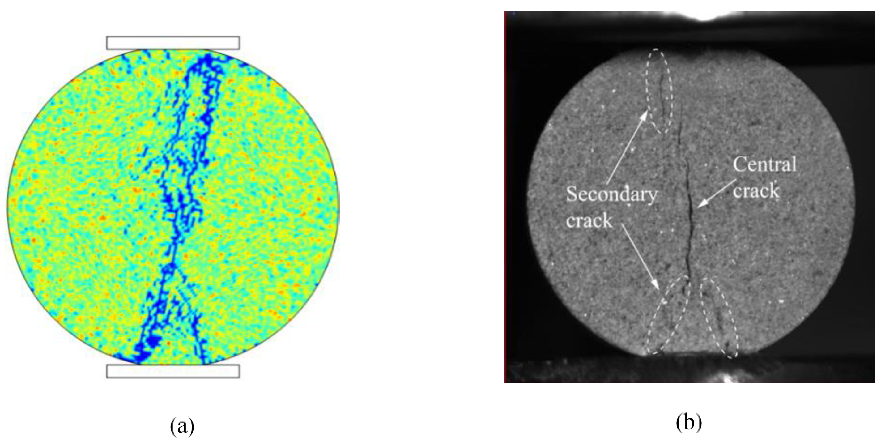
Once the peak load was reached, the damaged elements rapidly propagated, connected, and penetrated the specimen, resulting in a splitting crack along the loading direction. Moreover, the external load decreased sharply to a certain value. The entire failure process exhibited evident brittle characteristics consistent with the experiment. Pure tensile damage was also dominant in the final fracture, while shear damage, especially tension–shear damage, was rare and negligible. Figure 18 shows the final fracture mode along with the experimental results. The simulation results agree with the experimental results [51,52].
7. Conclusions
- A novel anisotropic damage model is proposed to improve the conventional isotropic damage model. It avoids the interpenetration of crack surfaces and unifies three forms of damage, which include pure tension, tension–shear, and compression–shear, as one smooth criterion. In addition, the shear damage evolution equation considers the equivalent shear strain on the failure face as the independent variable, which has a clearer physical meaning.
- The proposed anisotropic damage model is able to simulate the failure behavior of quasi-brittle materials more effectively. It can effectively simulate not only the mesoscale pure tension, tension shear, and compression shear damages but also the macroscale fracture mode and its evolution. It can also simulate the strength characteristics, including the peak and residual strengths, approximately.
- The simplified two-dimensional geometries were used to verify the proposed anisotropic damage model by comparison with a conventional damage model. However, the proposed anisotropic damage model and finite element implementation strategy proposed in this study also apply to three-dimensional, multi-scale, and multi-field coupling problems.
- Numerical tests of the failure behavior of quasi-brittle materials have the advantages of strong universality, convenience, flexibility, and repeatability compared with laboratory tests. In addition, they can provide mesoscale mechanical information that is difficult to observe in laboratory tests. However, owing to the limitations of the nonlinear solution method, numerical tests will take longer if there are more loading steps. The combination of numerical simulation and machine learning algorithms will help improve the efficiency of numerical tests better to serve the scientific research and teaching of quasi-brittle materials, which is also a follow-up research goal of the authors.
Author Contributions
Software, X.D.; formal analysis, P.J. and X.Z.; writing—original draft preparation, H.W.; writing—review and editing, B.Z.; supervision, S.X.; All authors have read and agreed to the published version of the manuscript.
Funding
This research was funded by [National Natural Science Foundation of China] grant number [51804323] and [Independent Innovation Research Program of China University of Petroleum (East China)] grant number [27RA2215005].
Acknowledgments
The authors thank the supports from the National Natural Science Foundation of China (grant no. 51804323) and the Independent Innovation Research Program of China University of Petroleum (East China) (grant no. 27RA2215005).
Conflicts of Interest
The authors declare no conflict of interest.
References
- Khosravani, M.R.; Silani, M.; Weinberg, K. Fracture studies of ultra-high performance concrete using dynamic Brazilian tests. Theor. Appl. Fract. Mech. 2018, 93, 302–310. [Google Scholar] [CrossRef]
- Yu, J.; Shang, X. Analysis of the influence of boundary pressure and friction on determining fracture toughness of shale using cracked Brazilian disc test. Eng. Fract. Mech. 2019, 212, 57–69. [Google Scholar] [CrossRef]
- Hokka, M.; Black, J.; Tkalich, D.; Fourmeau, M.; Kane, A.; Hoang, N.-H.; Li, C.C.; Chen, W.W.; Kuokkala, V.-T. Effects of strain rate and confining pressure on the compressive behavior of Kuru granite. Int. J. Impact Eng. 2016, 91, 183–193. [Google Scholar] [CrossRef]
- Ge, X.R.; Ren, J.X.; Pu, Y.B.; Ma, W. Real-in time CT test of the rock meso-damage propagation law. Sci. China Ser. E 2001, 44, 328–336. [Google Scholar] [CrossRef]
- Li, Y.Y.; Cui, H.Q.; Zhang, P.; Wang, D.K.; Wei, J.P. Three-dimensional visualization and quantitative characterization of coal fracture dynamic evolution under uniaxial and triaxial compression based on μCT scanning. Fuel 2020, 262, 116568. [Google Scholar] [CrossRef]
- Liu, Z.L.; Ma, C.D.; Wei, X.A.; Xie, W.B. Experimental study on mechanical properties and failure modes of pre-existing cracks in sandstone during uniaxial tension/compression testing. Eng. Fract. Mech. 2021, 255, 107966. [Google Scholar] [CrossRef]
- Yang, S.Q.; Huang, Y.H.; Tang, J.Z. Mechanical, acoustic, and fracture behaviors of yellow sandstone specimens under triaxial monotonic and cyclic loading. Int. J. Rock Mech. Min. 2020, 130, 104268. [Google Scholar] [CrossRef]
- Zhu, Q.Q.; Li, X.B.; Li, D.Y.; Ma, C.D. Experimental investigations of static mechanical properties and failure characteristics of damaged diorite after dynamic triaxial compression. Int. J. Rock Mech. Min. 2022, 153, 105106. [Google Scholar] [CrossRef]
- Valliappan, S.; Murti, V.; Zhang, W.H. Finite element analysis of anisotropic damage mechanics problems. Eng. Fract. Mech. 1990, 35, 1061–1071. [Google Scholar] [CrossRef]
- Xu, Y.; Yao, W.; Xia, K.W. Numerical study on tensile failures of heterogeneous rocks. J. Rock Mech. Geotech. 2020, 12, 54–62. [Google Scholar] [CrossRef]
- Zhang, W.; Guo, T.K.; Qu, Z.Q.; Wang, Z.Y. Research of fracture initiation and propagation in HDR fracturing under thermal stress from meso-damage perspective. Energy 2019, 178, 508–521. [Google Scholar] [CrossRef]
- Zhou, S.W.; Zhuang, X.Y.; Zhu, H.H.; Rabczuk, T. Phase field modelling of crack propagation, branching and coalescence in rocks. Theor. Appl. Fract. Mech. 2018, 96, 174–192. [Google Scholar] [CrossRef] [Green Version]
- Lu, X.X.; Cheng, L.; Tie, Y.; Hou, Y.L.; Zhang, C.Z. Crack propagation simulation in brittle elastic materials by a phase field method. Theor. Appl. Mech. Lett. 2019, 9, 339–352. [Google Scholar] [CrossRef]
- Fakhimi, A.; Villegas, T. Application of dimensional analysis in calibration of a discrete element model for rock deformation and fracture. Rock Mech. Rock Eng. 2007, 40, 193–211. [Google Scholar] [CrossRef]
- Qiu, J.D.; Li, D.Y.; Li, X.B.; Zhou, Z.L. Dynamic fracturing behavior of layered rock with different inclination angles in SHPB tests. Shock Vib. 2017, 2017, 7687802. [Google Scholar] [CrossRef] [Green Version]
- Ergenzinger, C.; Seifried, R.; Eberhard, P. A discrete element model to describe failure of strong rock in uniaxial compression. Granul. Matter 2011, 13, 341–364. [Google Scholar] [CrossRef]
- Shang, J.; Duan, K.; Gui, Y.; Zhao, Z. Numerical investigation of the direct tensile behavior of laminated and transversely isotropic rocks containing incipient bedding planes with different strengths. Comput. Geotech. 2017, 104, 373–388. [Google Scholar] [CrossRef] [Green Version]
- Li, K.H.; Yin, Z.Y.; Cheng, Y.M.; Cao, P.; Meng, J.J. Three-dimensional discrete element simulation of indirect tensile behaviour of a transversely isotropic rock. Int. J. Numer. Anal. Methods Geomech. 2020, 44, 1812–1832. [Google Scholar] [CrossRef]
- Zhang, X.D.; Bui, T.Q. A fictitious crack XFEM with two new solution algorithms for cohesive crack growth modeling in concrete structures. Eng. Comput. 2015, 32, 473–497. [Google Scholar] [CrossRef]
- Wu, J.Y.; Qiu, J.F.; Nguyen, V.P.; Mandal, T.K.; Zhang, L.J. Computational modeling of localized failure in solids: XFEM vs PF-CZM. Comput. Methods Appl. Mech. Eng. 2019, 345, 618–643. [Google Scholar] [CrossRef]
- Haddad, M.; Sepehrnoori, K. XFEM-Based CZM for the simulation of 3D multiple-cluster hydraulic fracturing in quasi-brittle shale formations. Rock Mech. Rock Eng. 2016, 49, 4731–4748. [Google Scholar] [CrossRef]
- Peixoto, R.G.; Ribeiro, G.O.; Pitangueira, R.L.S. A boundary element method formulation for quasi-brittle material fracture analysis using the continuum strong discontinuity approach. Eng. Fract. Mech. 2018, 202, 47–74. [Google Scholar] [CrossRef]
- Ooi, E.T.; Natarajan, S.; Song, C.; Ooi, E.H. Crack propagation modelling in concrete using the scaled boundary finite element method with hybrid polygon-quadtree meshes. Int. J. Fract. 2017, 203, 135–157. [Google Scholar] [CrossRef]
- Chen, C.S.; Pan, E.; Amadei, B. Fracture mechanics analysis of cracked discs of aniso-tropic rock using the boundary element method. Int. J. Rock Mech. Min. 1998, 35, 195–218. [Google Scholar] [CrossRef]
- Crouch, S.L. Analysis of Stresses and Displacements around Underground Excavations: An Application of the Displacement Discontinuity Method, 2nd Printing; Geomechanics Report; University of Minnesota: Minneapolis, MN, USA, 1980. [Google Scholar]
- Kuriyama, K.; Mizuta, Y. Three-dimensional elastic analysis by the displacement discontinuity method with boundary division into triangular leaf elements. Int. J. Rock Mech. Min. 1993, 30, 111–123. [Google Scholar] [CrossRef]
- Marji, M.F. Numerical analysis of quasi-static crack branching in brittle solids by a modified displacement discontinuity method. Int. J. Solids Struct. 2014, 51, 1716–1736. [Google Scholar] [CrossRef] [Green Version]
- Abdollahipour, A.; Marji, M.F.; Bafghi, A.Y.; Gholamnejad, J. Time-dependent crack propagation in a poroelastic medium using a fully coupled hydromechanical displacement discontinuity method. Int. J. Fract. 2016, 199, 71–87. [Google Scholar] [CrossRef]
- Xiroudakis, G.; Stavropoulou, M.; Exadaktylos, G. Three-dimensional elastic analysis of cracks with the g2 constant displacement discontinuity method. Int. J. Numer. Anal. Methods Geomech. 2019, 43, 2355–2382. [Google Scholar] [CrossRef]
- Tang, C.A.; Tang, S.B. Applications of rock failure process analysis (RFPA) method. J. Rock Mech. Geotech. 2011, 3, 352–372. [Google Scholar] [CrossRef]
- Li, G.; Tang, C.A. A statistical meso-damage mechanical method for modeling trans-scale progressive failure process of rock. Int. J. Rock Mech. Min. 2015, 74, 133–150. [Google Scholar] [CrossRef]
- Sun, C.; Zheng, H.; Liu, W.D.; Lu, W.T. Numerical investigation of complex fracture network creation by cyclic pumping. Eng. Fract. Mech. 2020, 233, 107103. [Google Scholar] [CrossRef]
- Sun, B.; Liu, X.J.; Xu, Z.D. A novel physical continuum damage model for the finite element simulation of crack growth mechanism in quasi-brittle geomaterials. Theor. Appl. Fract. Mech. 2021, 114, 103030. [Google Scholar] [CrossRef]
- Miehe, C.; Hofacker, M.; Schänzel, L.-M.; Aldakheel, F. Phase field modeling of fracture in multi-physics problems. Part II. Coupledbrittle-to-ductile failure criteria and crack propagation in thermo-elastic–plastic solids. Comput. Methods Appl. Mech. Eng. 2015, 294, 486–522. [Google Scholar] [CrossRef]
- Staroselsky, A.; Acharya, R.; Cassenti, B. Phase field modeling of fracture and crack growth. Eng. Fract. Mech. 2019, 205, 268–284. [Google Scholar] [CrossRef]
- Noll, T.; Kuhn, C.; Olesch, D.; Müller, R. 3D phase field simulations of ductile fracture. GAMM-Mitt. 2020, 43, e202000008. [Google Scholar] [CrossRef] [Green Version]
- Wei, C.H.; Zhu, W.C.; Chen, S.K.; Ranjith, P.G. A coupled thermal–hydrological–mechanical damage model and its numerical simulations of damage evolution in APSE. Materials 2016, 9, 841. [Google Scholar] [CrossRef] [Green Version]
- Wang, Z. A Modified Mohr Coulomb Criterion for Rocks with Smooth Tension Cut-off. IOP Conf. Ser. Earth Environ. Sci. 2020, 525, 012027. [Google Scholar] [CrossRef]
- Zhou, G.L.; Xu, T.; Heap, M.J.; Meredith, P.G.; Mitchell, T.M.; Sesnic, A.S.Y.; Yuan, Y. A three-dimensional numerical meso-approach to modeling time- independent deformation and fracturing of brittle rocks. Comput Geotech. 2020, 117, 103274. [Google Scholar] [CrossRef]
- She, C.X.; Liu, J. Two-parameter parabolic-type yield criterion based on Mohr strength theory. Eng. J. Wuhan Univ. 2008, 41, 33–36. [Google Scholar]
- Gill, S. A damage model for the frictional shear failure of brittle materials in compression. Comput. Methods Appl. Mech. Eng. 2021, 385, 114048. [Google Scholar] [CrossRef]
- Murakami, S. Continuum Damage Mechanics: A Continuum Mechanics Approach to the Analysis of Damage and Fracture; Springer Science & Business Media: Nagoya, Japan, 2012; pp. 19–20. [Google Scholar]
- Tang, S.; Zhang, H.; Tang, C.; Liu, H. Numerical model for the cracking behavior of heterogeneous brittle solids subjected to thermal shock. Int. J. Solids Struct. 2016, 80, 520–531. [Google Scholar] [CrossRef]
- Chen, Z.H.; Tham, L.G.; Yeung, M.R.; Xie, H. Confinement effects for damage and failure of brittle rocks. Int. J. Rock Mech. Min. 2006, 43, 1262–1269. [Google Scholar] [CrossRef]
- Guo, T.K.; Du, Z.M. Meso-numerical simulation of rock triaxial compression based on the damage model. Conf. Ser. Earth Environ. Sci. 2021, 687, 012134. [Google Scholar] [CrossRef]
- Zong, Y.J.; Han, L.J.; Wei, J.J.; Wen, S.Y. Mechanical and damage evolution properties of sandstone under triaxial compression. Int. J. Min. Sci. Technol. 2016, 26, 601–607. [Google Scholar] [CrossRef]
- Yao, M.D.; Rong, G.; Zhou, C.B.; Peng, J. Effects of Thermal Damage and Confining Pressure on the Mechanical Properties of Coarse Marble. Rock Mech. Rock Eng. 2016, 49, 2043–2054. [Google Scholar] [CrossRef]
- Zhang, J.C.; Lin, Z.N.; Dong, B.; Guo, R.X. Triaxial Compression Testing at Constant and Reducing Confining Pressure for the Mechanical Characterization of a Specific Type of Sandstone. Rock Mech. Rock Eng. 2021, 54, 1999–2012. [Google Scholar] [CrossRef]
- Benz, T.; Schwab, R.; Kauther, R.A.; Vermeer, P.A. A Hoek–Brown criterion with intrinsic material strength factorization. Int. J. Rock Mech. Min. 2008, 45, 210–222. [Google Scholar] [CrossRef]
- Khosravani, M.R.; Friebertshäuser, K.; Weinberg, K. On the use of peridynamics in fracture of ultra-high performance concrete. Mech. Res. Commun. 2022, 123, 103899. [Google Scholar] [CrossRef]
- You, M.; Su, C. Experimental study on split test with flattened disk and tensile strength of rock. Chin. J. Rock Mech. Eng. 2004, 23, 3106–3112. [Google Scholar]
- Yan, Z.L.; Dai, F.; Liu, Y.; Wei, M.D.; You, W. New insights into the fracture mechanism of flattened Brazilian disc specimen using digital image correlation. Eng. Fract. Mech. 2021, 252, 107810. [Google Scholar] [CrossRef]
Figure 1.
Two-parameter parabolic-type yield envelope and Mohr circles.
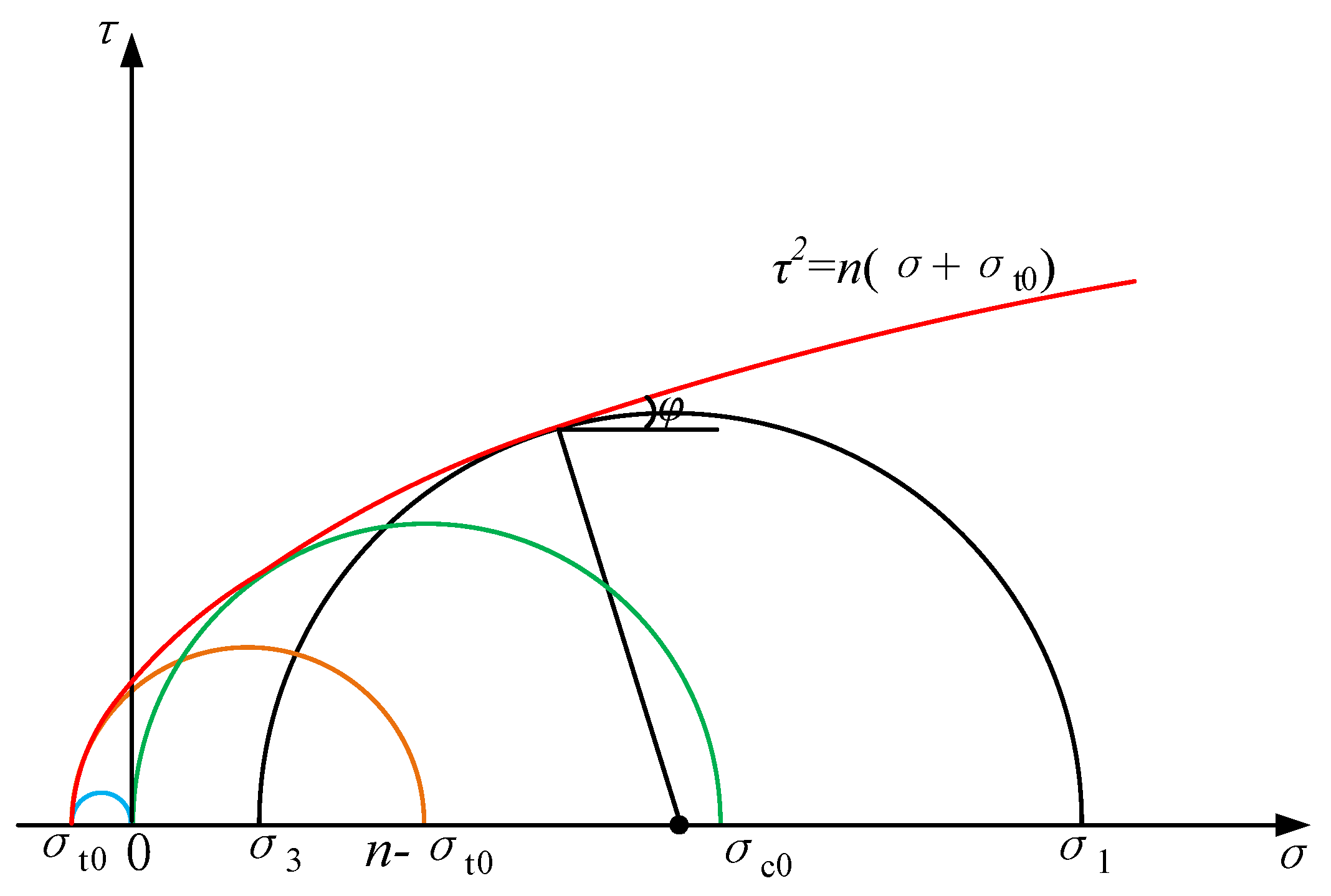
Figure 2.
Stress–strain relationship under uniaxial tension for elastic–brittle tensile damage.
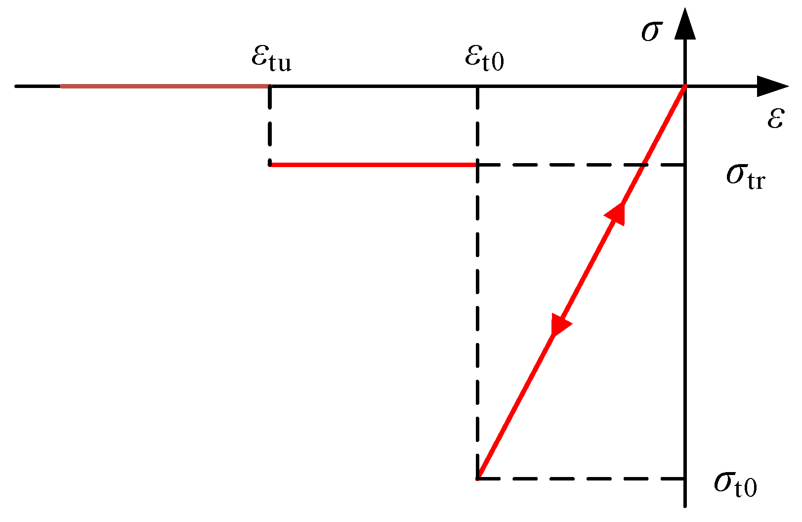
Figure 3.
Shear stress–shear strain relation for elastic–brittle–plastic shear damage.
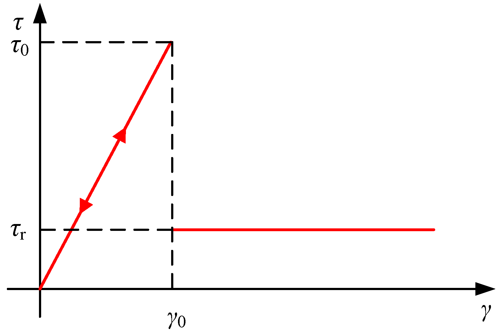
Figure 4.
Calculation flowchart of numerical simulation.
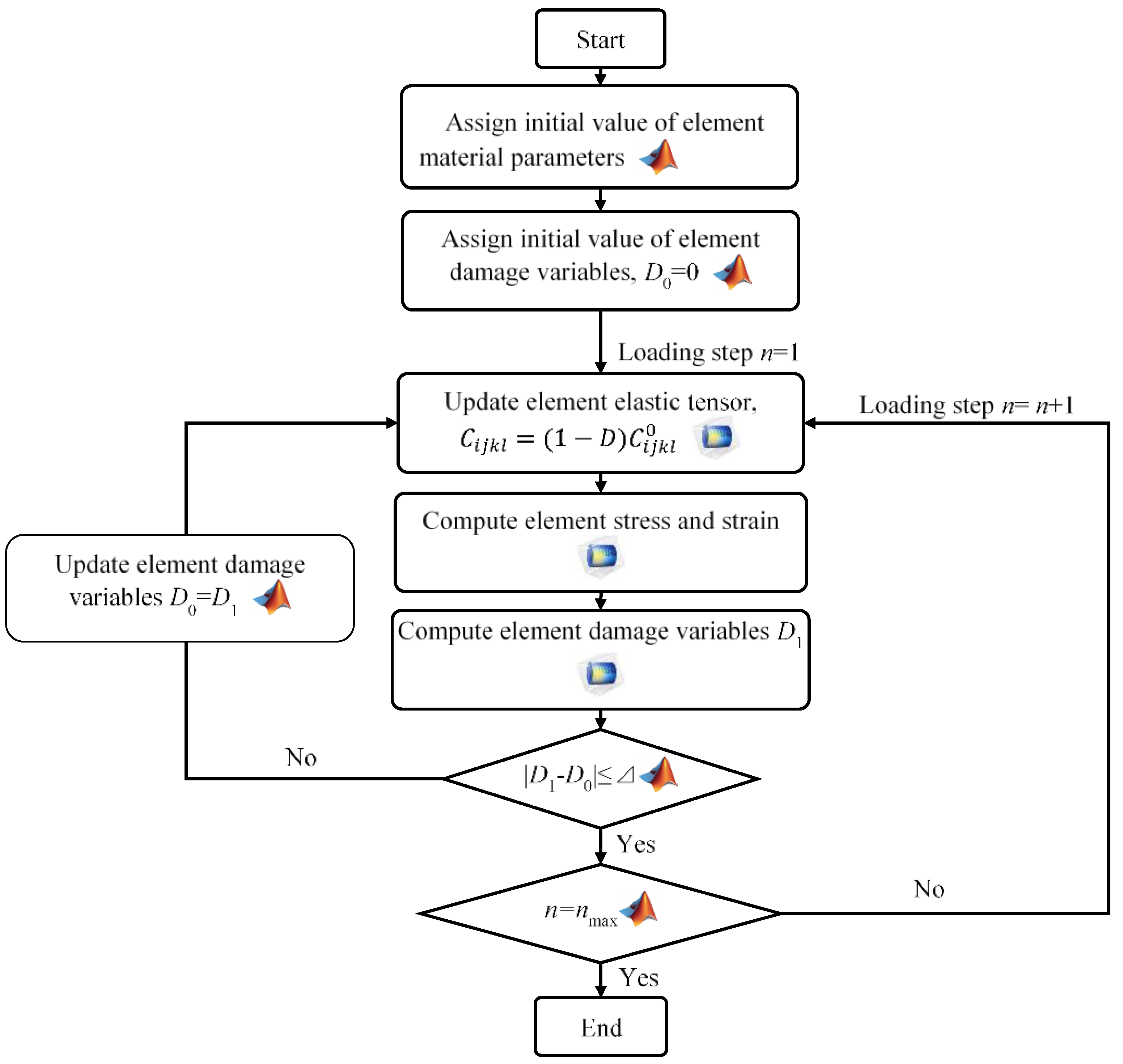
Figure 5.
Finite element model of the test case, (a) model geometry; (b) mesh grids.
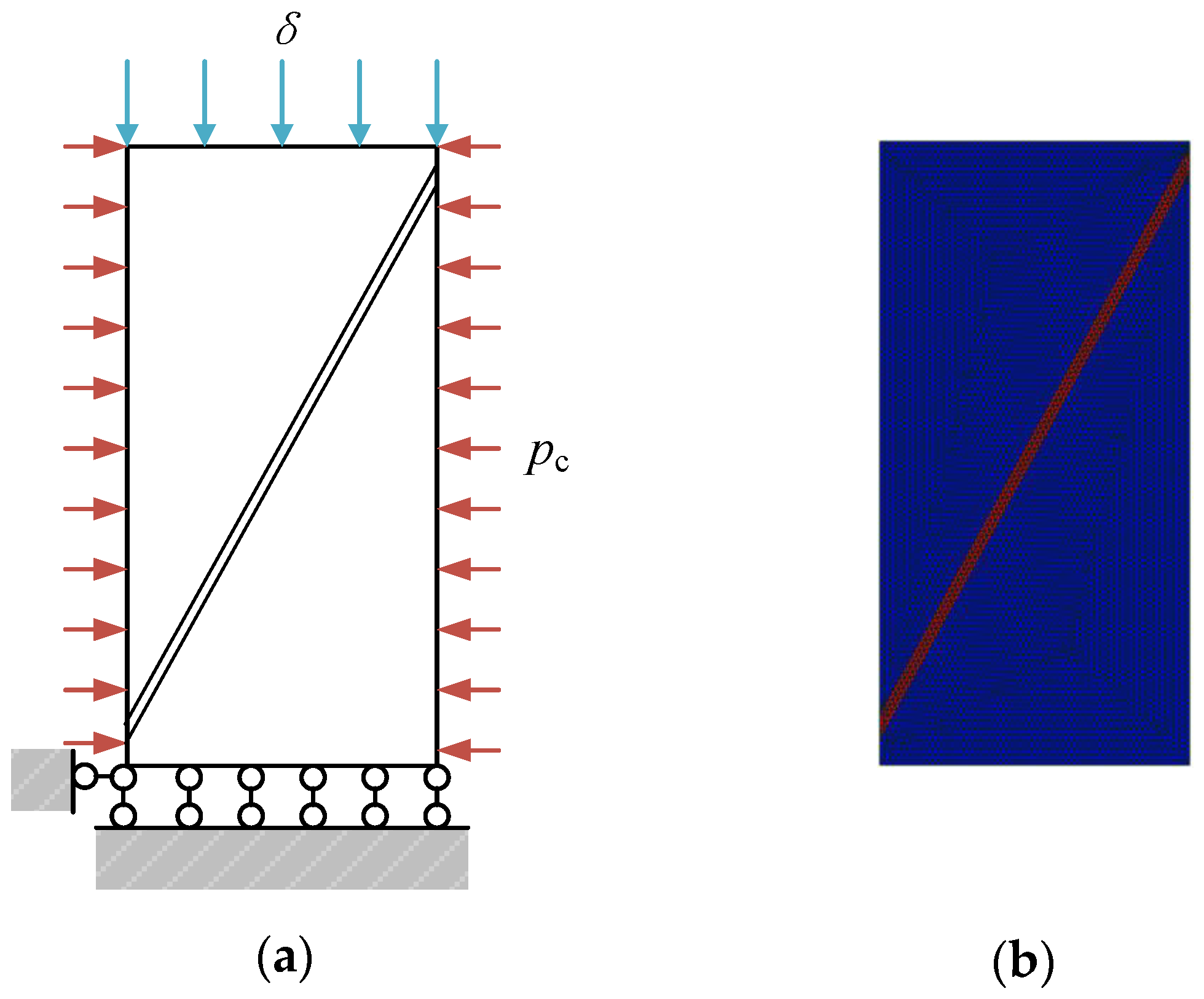
Figure 6.
Comparison of failure modes (a) anisotropic damage model, pc = 0 MPa; (b) anisotropic damage model, pc = 10 MPa; (c) isotropic damage model, pc = 0 MPa; (d) isotropic damage model, pc = 10 MPa.
Figure 6.
Comparison of failure modes (a) anisotropic damage model, pc = 0 MPa; (b) anisotropic damage model, pc = 10 MPa; (c) isotropic damage model, pc = 0 MPa; (d) isotropic damage model, pc = 10 MPa.
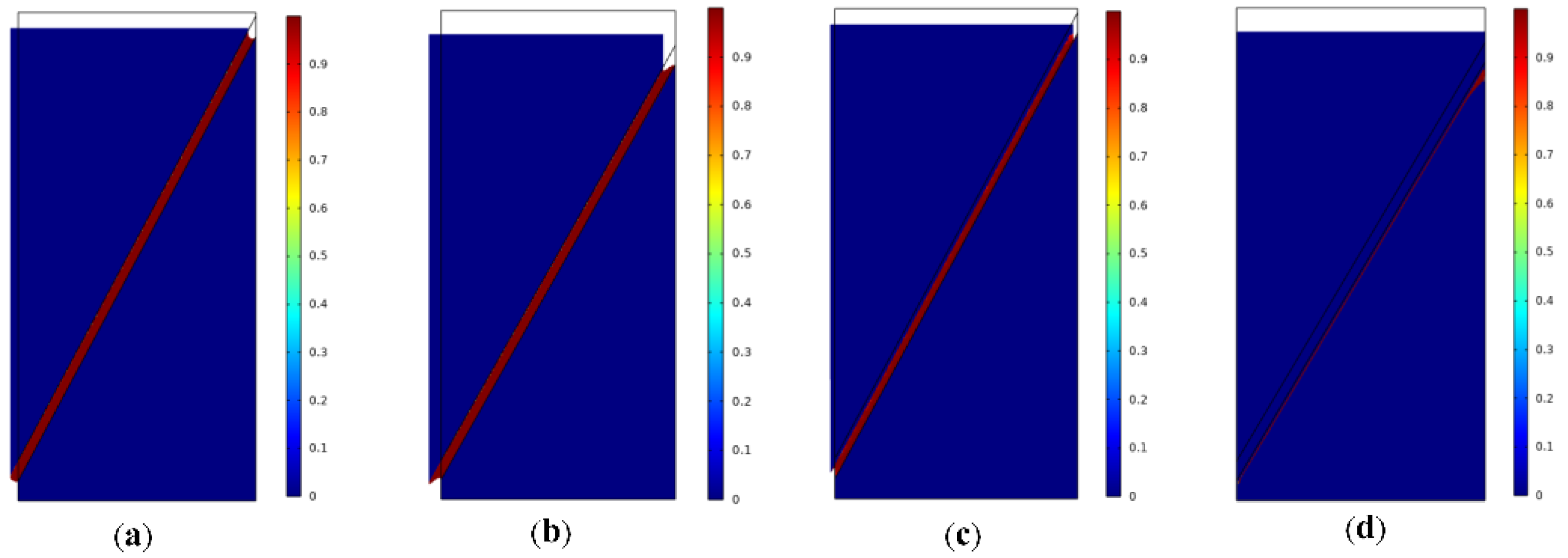
Figure 7.
Finite element model of the rock specimen in compression tests, (a) model geometry; (b) mesh grids and initial elastic modulus.
Figure 7.
Finite element model of the rock specimen in compression tests, (a) model geometry; (b) mesh grids and initial elastic modulus.
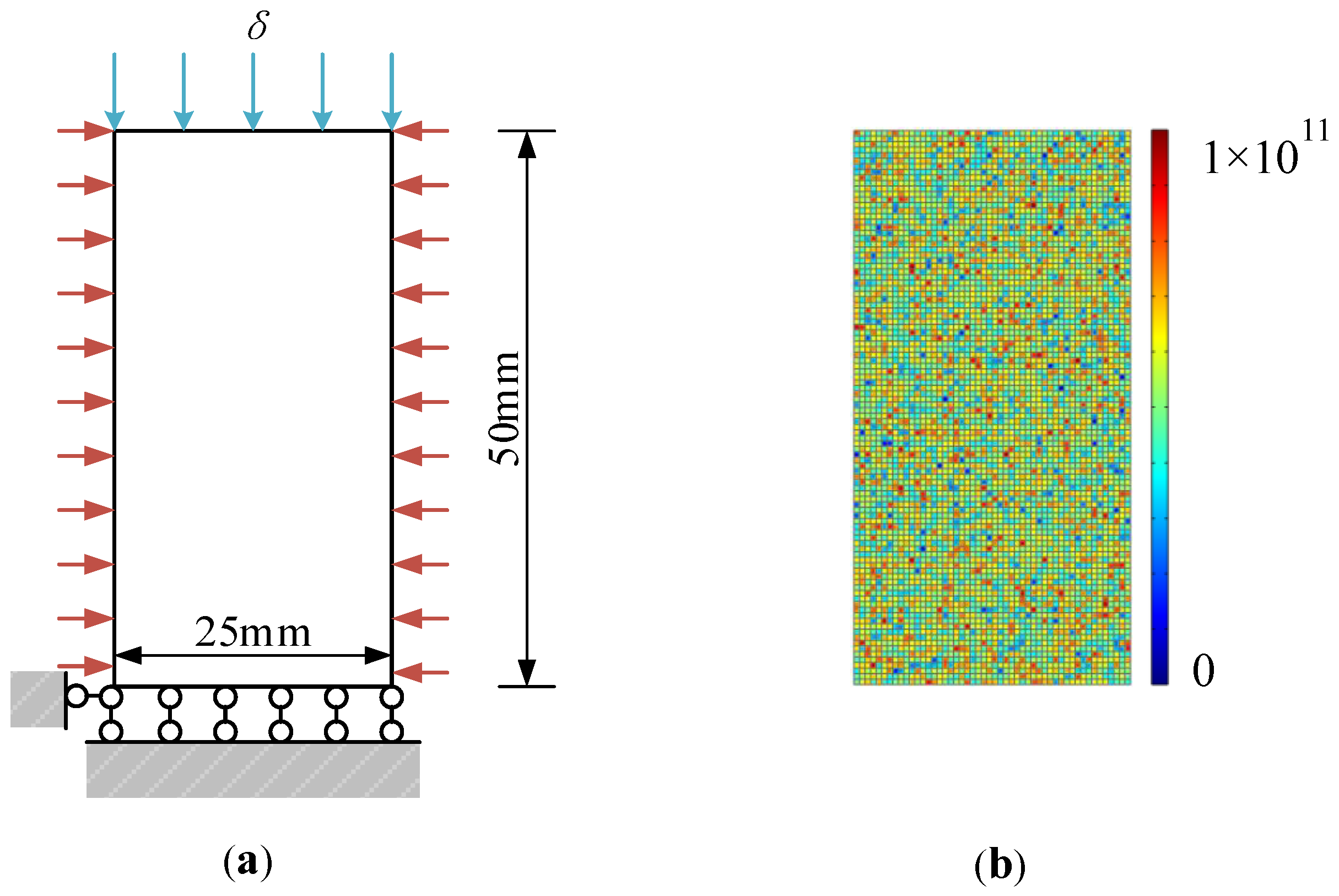
Figure 8.
Failure process of rock specimen under axial compression, pc = 0 MPa, (a) damage variable; (b) damage mode.
Figure 8.
Failure process of rock specimen under axial compression, pc = 0 MPa, (a) damage variable; (b) damage mode.

Figure 9.
Failure process of rock specimen under biaxial compression, pc = 10 MPa, (a) damage variable; (b) damage mode.
Figure 9.
Failure process of rock specimen under biaxial compression, pc = 10 MPa, (a) damage variable; (b) damage mode.
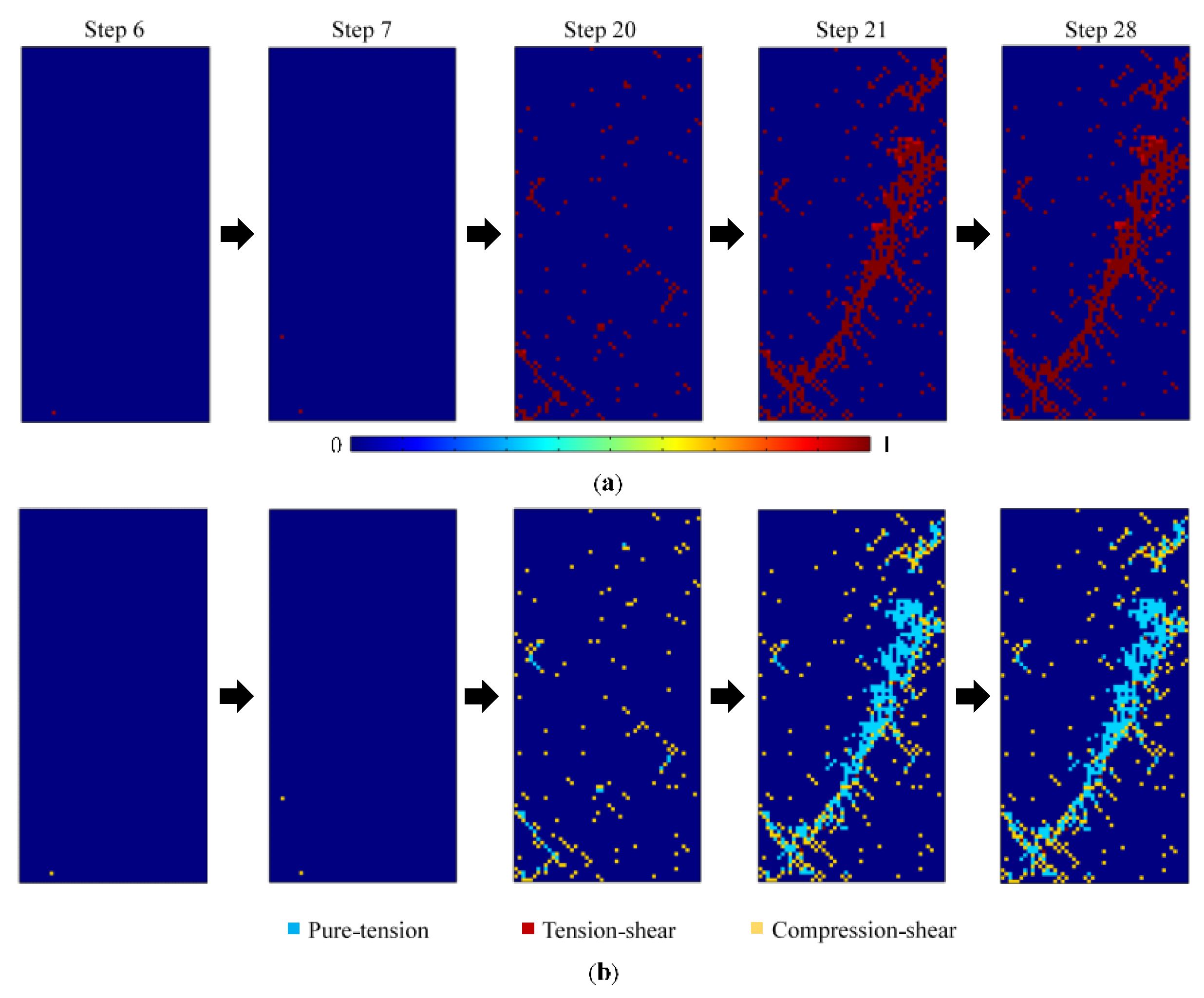
Figure 10.
Failure process of rock specimen under biaxial compression, pc = 20 MPa, (a) damage variable; (b) damage mode.
Figure 10.
Failure process of rock specimen under biaxial compression, pc = 20 MPa, (a) damage variable; (b) damage mode.

Figure 11.
Failure process of rock specimen under biaxial compression, pc = 40 MPa, (a) damage variable; (b) damage mode.
Figure 11.
Failure process of rock specimen under biaxial compression, pc = 40 MPa, (a) damage variable; (b) damage mode.
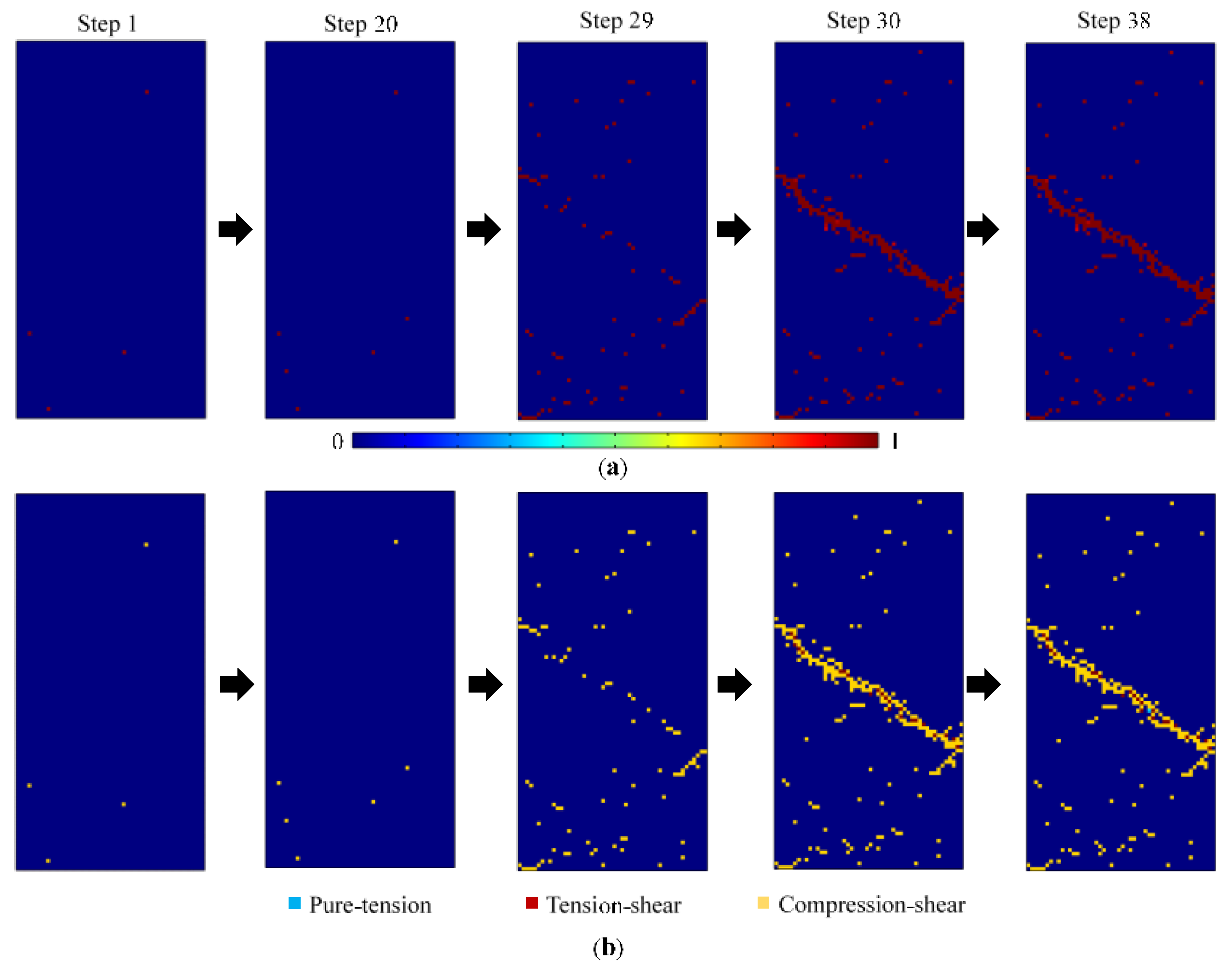
Figure 12.
Fracture modes of rock specimens under different confining pressures, (a) simulated results of elastic modulus; (b) experimental results, reprinted with permission from [46], 2016 Elsevier.
Figure 12.
Fracture modes of rock specimens under different confining pressures, (a) simulated results of elastic modulus; (b) experimental results, reprinted with permission from [46], 2016 Elsevier.
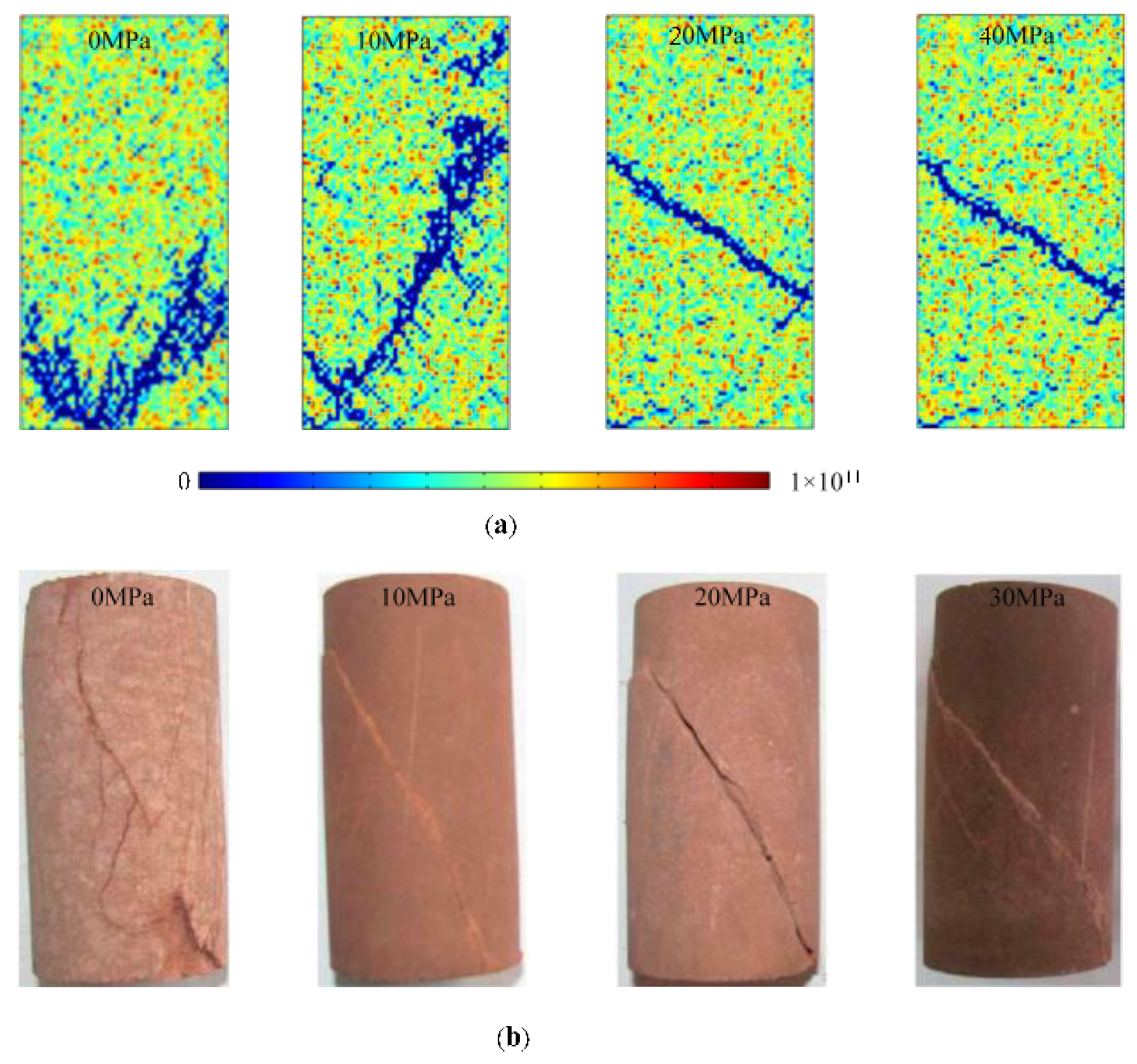
Figure 13.
Stress–strain curves under different confining pressures.
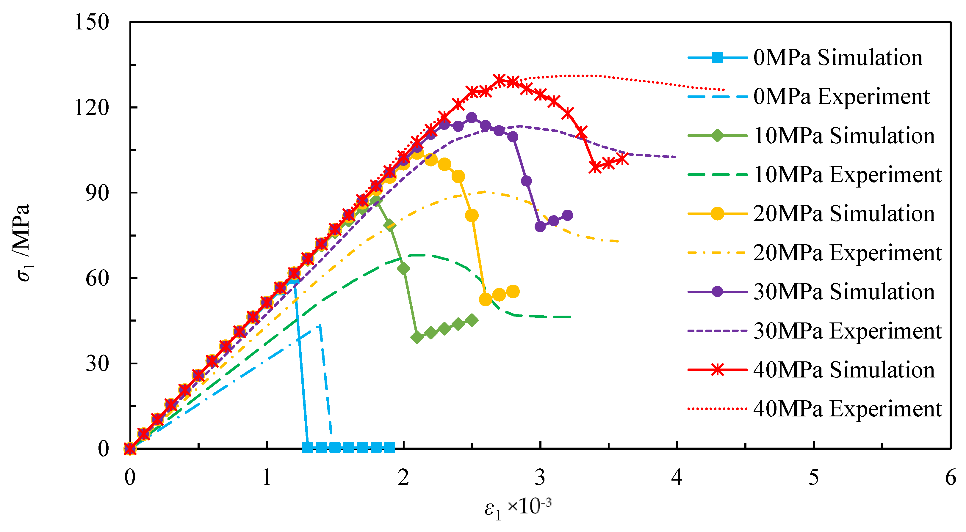
Figure 14.
Peak and residual strengths under different confining pressures.
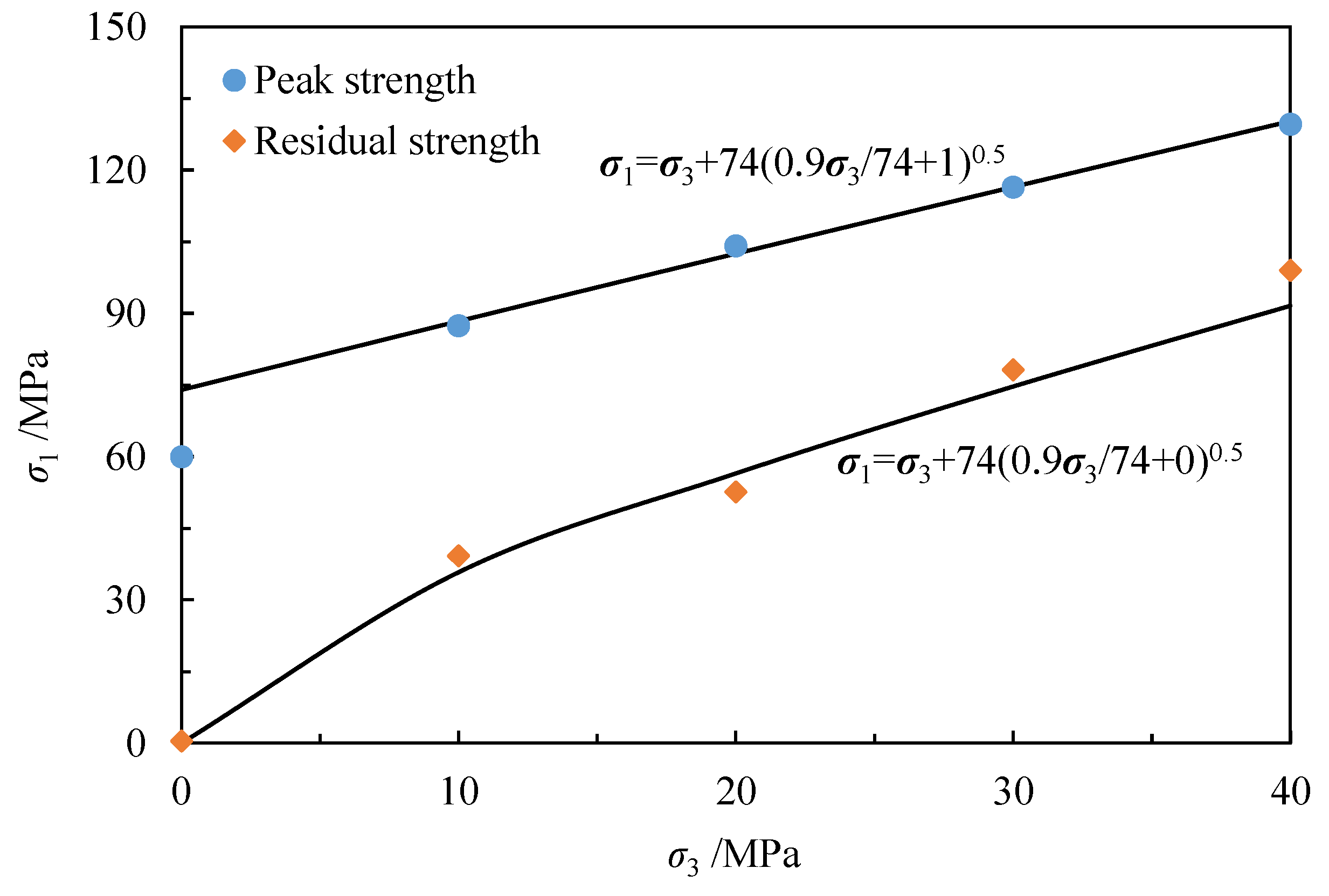
Figure 15.
Finite element model of the rock specimen in Brazilian tensile tests, (a) model geometry; (b) mesh grids and initial elastic modulus.
Figure 15.
Finite element model of the rock specimen in Brazilian tensile tests, (a) model geometry; (b) mesh grids and initial elastic modulus.
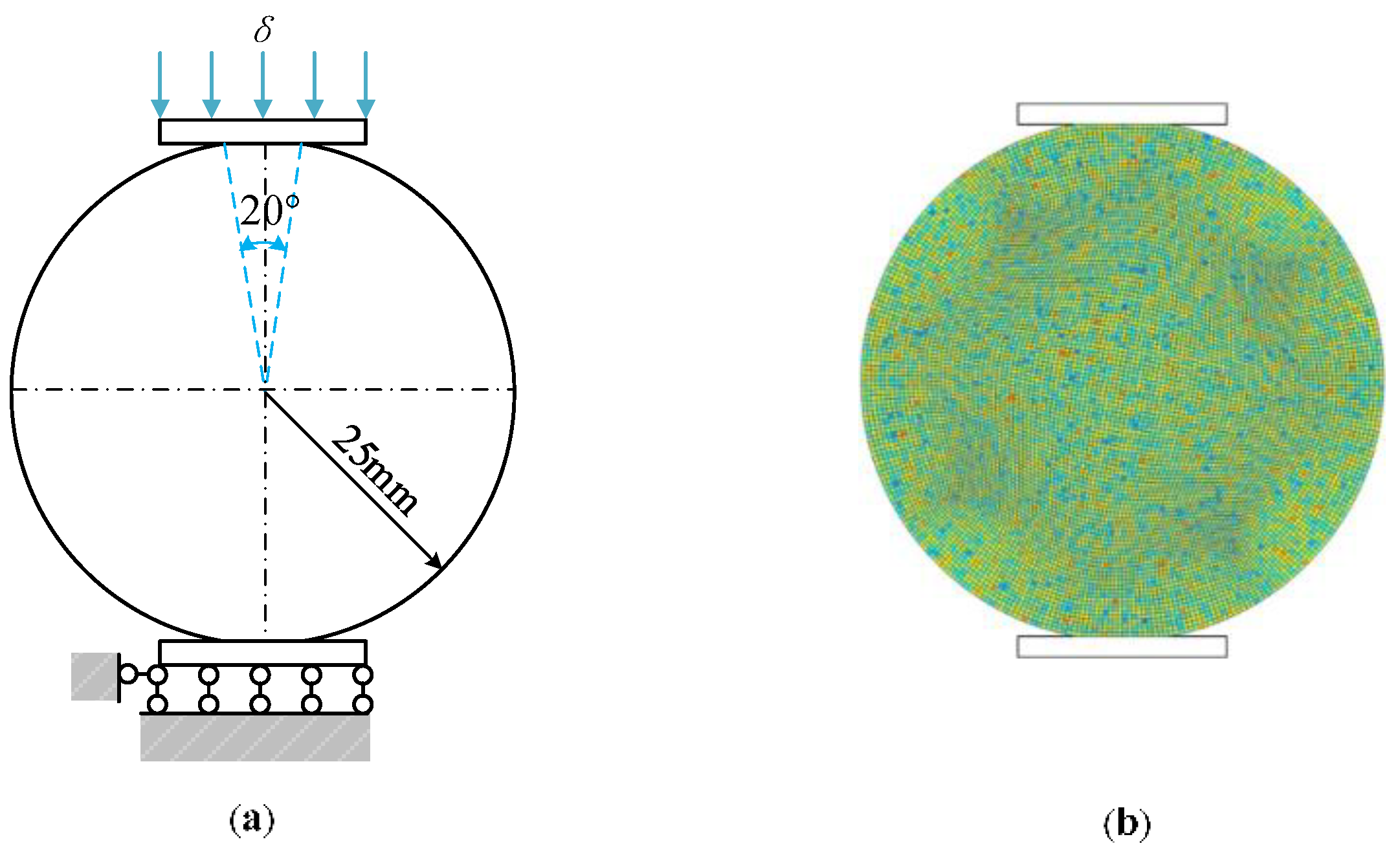
Figure 16.
Failure processes of disc specimen, (a) damage variable; (b) damage mode.
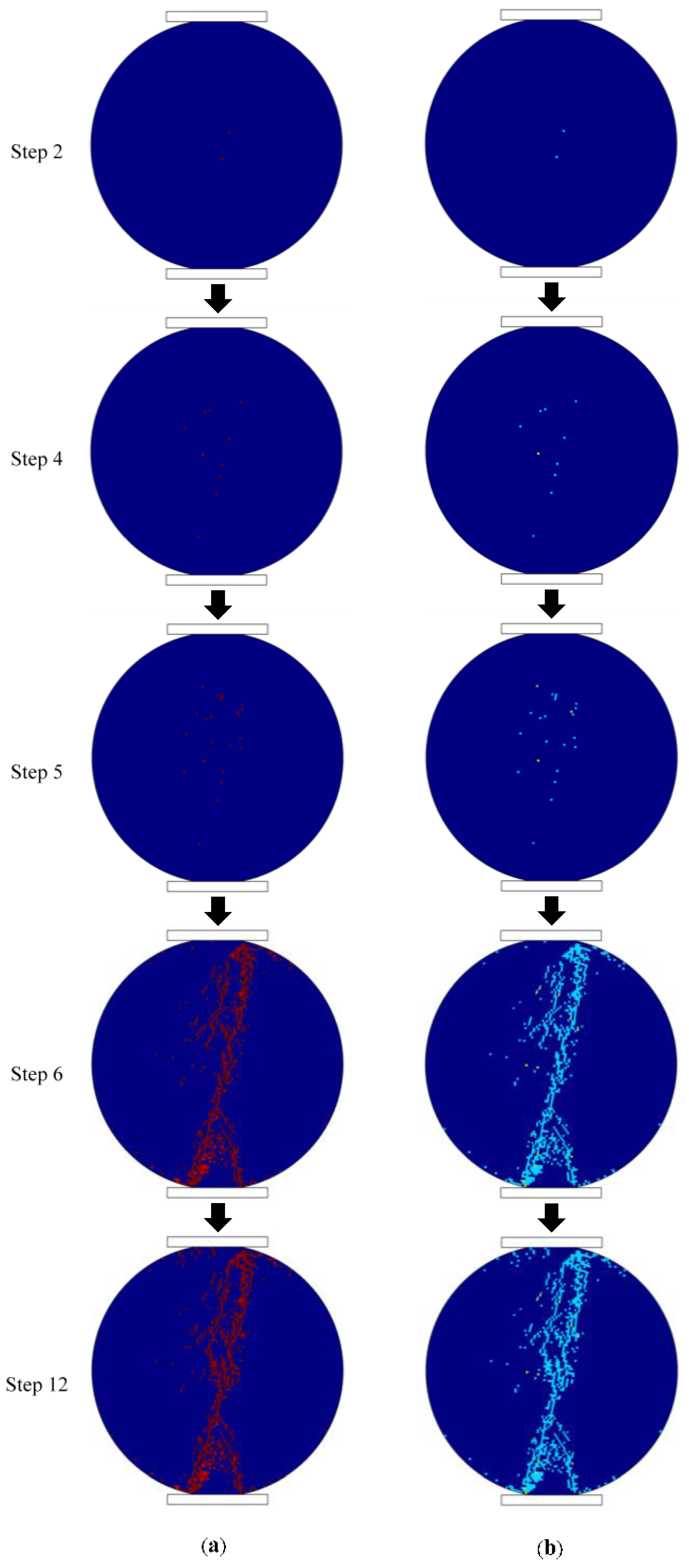
Figure 17.
Load–displacement curve of Brazilian splitting test.
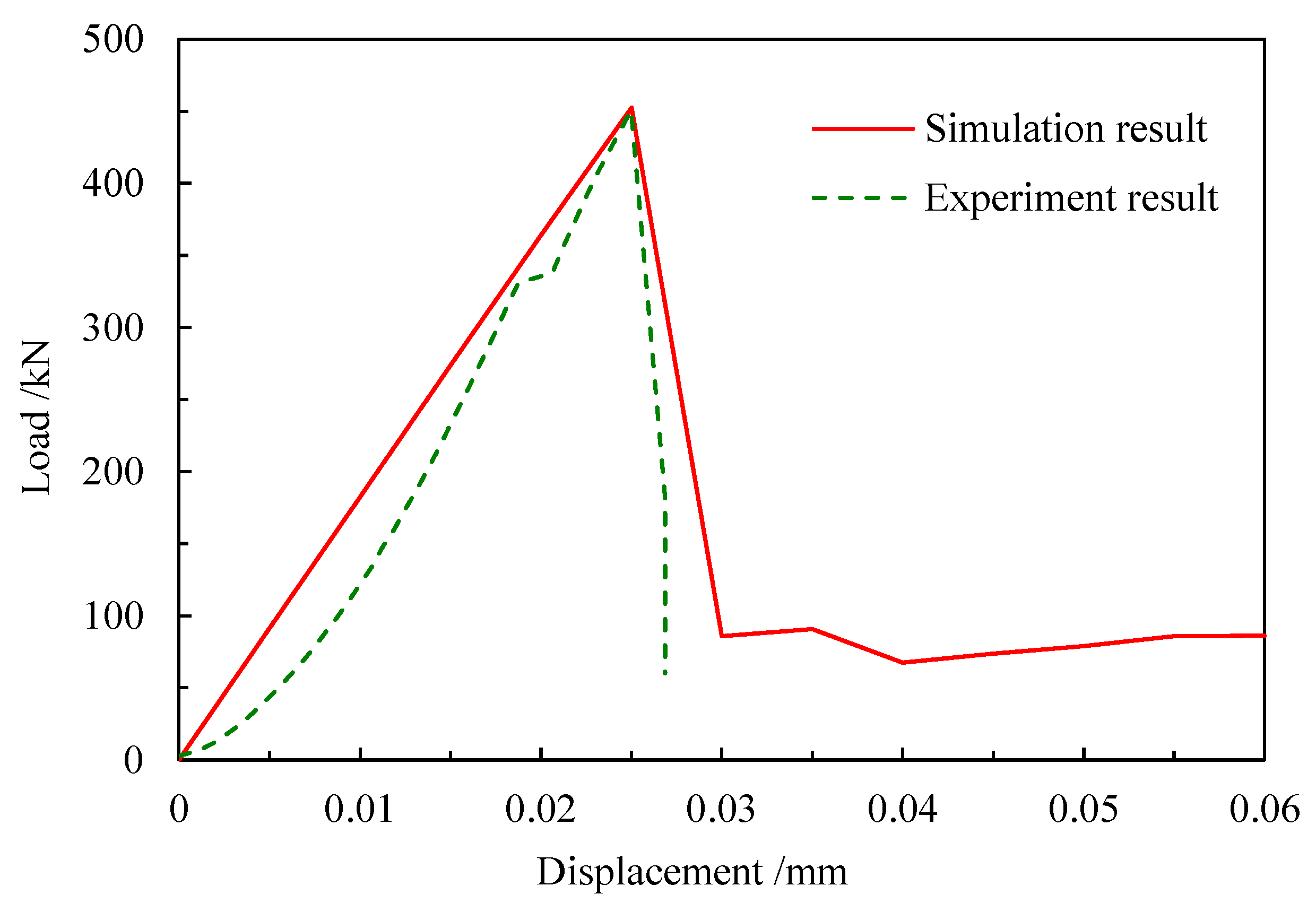
Figure 18.
Fracture mode of disc specimen, (a) simulated result of elastic modulus; (b) experimental result, reprinted with permission from [52], 2021 Elsevier.
Figure 18.
Fracture mode of disc specimen, (a) simulated result of elastic modulus; (b) experimental result, reprinted with permission from [52], 2021 Elsevier.
Publisher’s Note: MDPI stays neutral with regard to jurisdictional claims in published maps and institutional affiliations. |
© 2022 by the authors. Licensee MDPI, Basel, Switzerland. This article is an open access article distributed under the terms and conditions of the Creative Commons Attribution (CC BY) license (https://creativecommons.org/licenses/by/4.0/).
Share and Cite
MDPI and ACS Style
Wang, H.; Zhou, B.; Xue, S.; Deng, X.; Jia, P.; Zhu, X. An Anisotropic Damage Model of Quasi-Brittle Materials and Its Application to the Fracture Process Simulation. Appl. Sci. 2022, 12, 12073. https://doi.org/10.3390/app122312073
AMA Style
Wang H, Zhou B, Xue S, Deng X, Jia P, Zhu X. An Anisotropic Damage Model of Quasi-Brittle Materials and Its Application to the Fracture Process Simulation. Applied Sciences. 2022; 12(23):12073. https://doi.org/10.3390/app122312073
Chicago/Turabian StyleWang, Haijing, Bo Zhou, Shifeng Xue, Xuejing Deng, Peng Jia, and Xiuxing Zhu. 2022. "An Anisotropic Damage Model of Quasi-Brittle Materials and Its Application to the Fracture Process Simulation" Applied Sciences 12, no. 23: 12073. https://doi.org/10.3390/app122312073
Note that from the first issue of 2016, this journal uses article numbers instead of page numbers. See further details here.