Article

Long Short-Term Memory-Based Methodology for Predicting Carbonation Models of Reinforced Concrete Slab Bridges: Case Study in South Korea

Department of Structural Engineering Research, Korea Institute of Civil Engineering and Building Technology, Goyang 10223, Republic of Korea
*
Author to whom correspondence should be addressed.
Appl. Sci. 2022, 12(23), 12470; https://doi.org/10.3390/app122312470
Submission received: 17 November 2022 / Revised: 2 December 2022 / Accepted: 2 December 2022 / Published: 6 December 2022
(This article belongs to the Topic AI Enhanced Civil Infrastructure Safety)

Abstract

:

Featured Application

The proposed methodology creates LSTM-based carbonation models using the data from existing bridges. The proposed methodology and results can help bridge managers to conduct preventive maintenance.

Abstract

Reinforced concrete slab (RCS) bridges deteriorate because of exposure to environmental factors over time, resulting in reduced durability. Particularly, the carbonation of RCS bridges corrodes the rebars and reduces the strength. However, carbonation models derived from short-term experiments exhibit low reliability with respect to existing bridges. Therefore, a long short-term memory (LSTM)-based methodology was developed in this study for generating carbonation models using existing bridge inspection reports. The proposed methodology trains the LSTM model by combining data extracted from reports and local environmental data. The learning process uses padding and masking methods to consider the history of environmental data. A case study was performed to validate the proposed method in three different regions of Korea. The results verified that the coefficient of determination of the proposed method was higher than those of the existing carbonation models and other regression analyses. Therefore, the developed methodology can be used for predicting regional carbonation models using the data from existing bridges.

1. Introduction

Bridge deterioration is characterized by a decline in durability, structural safety, and function over time, which can lead to serious safety issues. Particularly, the material deterioration of reinforced concrete reduces its durability owing to the infiltration of environmental substances, such as carbon dioxide and seawater. Carbon dioxide is an aggressive substance that penetrates the pores inside the concrete and reacts with the hydrated calcium compound to modify it. This phenomenon is referred to as concrete carbonation and is an indicator for determining the lifespan of structures. Carbonation activates the penetration of other chlorides and the chemical corrosion of concrete rebars. Chemical corrosion negatively affects the stability of bridges, which can cause accidents. Most maintenance methods aim to observe bridge deterioration and maintain minimum performance for accident prevention. However, these maintenance methods require a significant budget as the repairs occur after deterioration. Therefore, several researchers have proposed preventative maintenance methods, wherein the deterioration and performance degradation of bridges are predicted in advance to ensure effective economic management.
Several studies have calculated the carbonation of bridge structures [1,2]. Typically, carbonation occurs slowly and is analyzed using accelerated testing. These studies aimed to regress the short-term carbonation of concrete within one year. The short-term carbonation model is most affected by the mixing ratio and curing time of the concrete [3]. However, field investigations of the natural environment remain scarce despite numerous experimental and theoretical studies. In general, three limitations are observed in applying the carbonation model to actual bridges. First, the actual reinforced concrete bridge over 10 years is significantly affected by environmental variables from a long-term perspective. However, the experimental environment estimates the weights for the environmental parameters because it exposes the concrete only for a short period. The low weighting of environmental variables can deteriorate the performance of long-term carbonation models. Second, most of the design data for bridges older than 30 years have been lost. Moreover, the mixing and curing periods of the concrete set in the design stage change owing to errors during the actual construction. These problems prevent the calculation of constants of several developed carbonation models, thereby reducing their usefulness. Third, environmental conditions change because of continuous changes in climate. The increase in the average temperature caused by global warming and the increasing trend of atmospheric CO2 concentration (278 to 400 ppm during the industrial period [4]) may accelerate the carbonation of cement and concrete [5,6]. Owing to these limitations, establishing a mathematical calculation model to accurately reflect the various factors of complex carbonation is difficult. Therefore, a novel approach that differs from the existing theories is required.
Artificial neural network (ANN) algorithms have been applied to solve several complex problems in concrete technology [7,8,9,10,11,12,13], and ANN-based models are widely used for estimating specific carbonation depths [14,15,16,17,18,19]. Although most studies consider certain influencing parameters, environmental conditions are not considered because of continuous changes in climate [20,21]. ANN models including climate change will produce highly accurate carbonation models, but further studies are needed [22,23]. Therefore, this study aims to develop an ANN-based methodology to predict the long-term carbonation model of field bridges considering climate change. The generated carbonation model considers climate change using data extracted from inspection reports. The dataset was constructed from the carbonation data of slabs, girders, piers, and abutments, which are major members of reinforced concrete slab (RCS) bridges in Korea. Additionally, environmental data were collected based on the different regions in Korea. The carbonation algorithm obtained the environmental data from the year of construction to the time of measurement as time series data; the analysis was performed using a long short-term memory (LSTM) model. In other words, the LSTM model was trained using a carbonation algorithm developed based on the environmental data from construction to inspection. During the analysis, the timestep non-uniformity problem was solved according to the usage period via padding and masking methods. The results verified that the proposed methodology exhibited higher accuracy than other carbonation models. The results of this study contribute to the development of an ANN-based carbonation model to consider long-term carbonation.

2. Literature Review

2.1. Concrete Carbonation Model
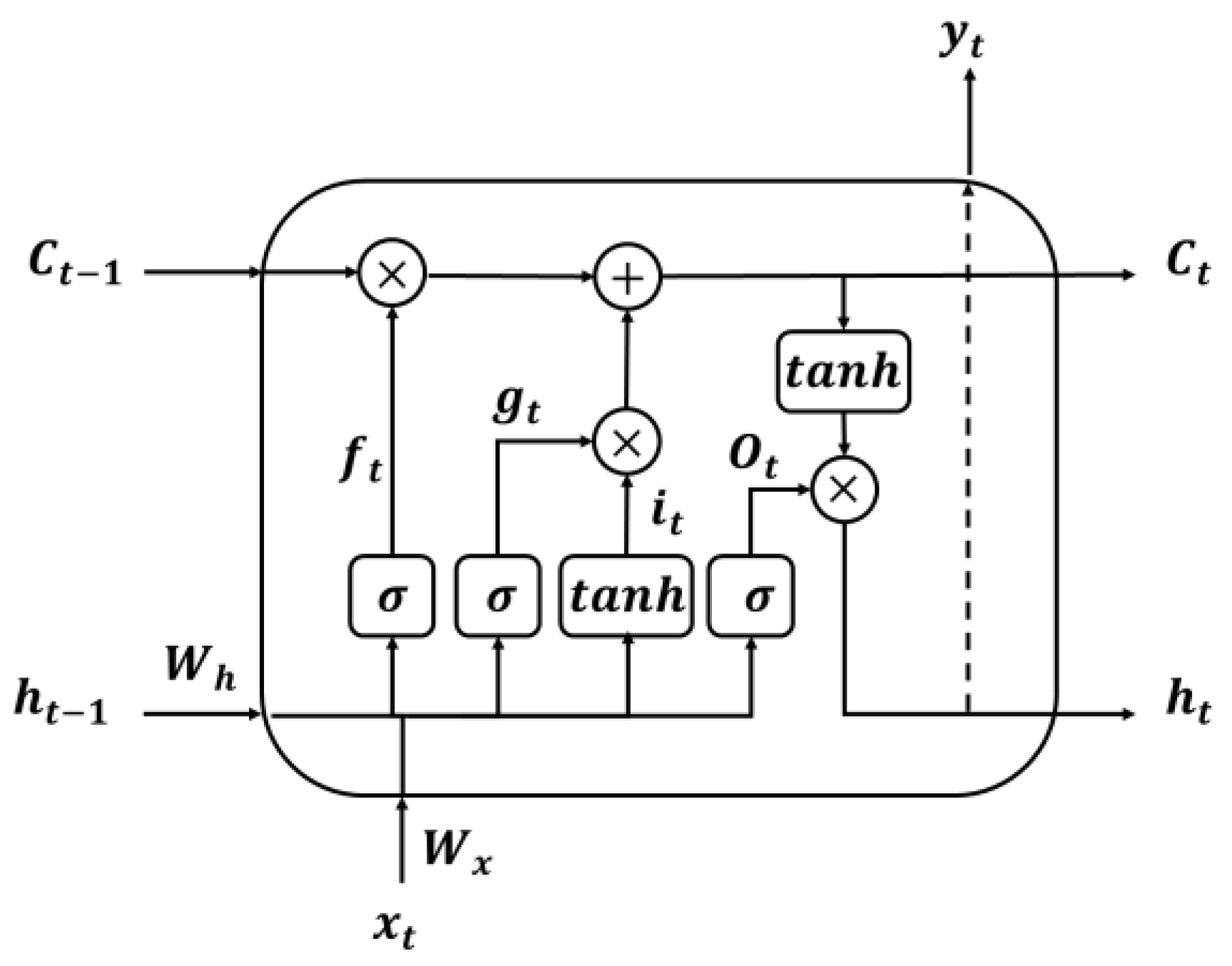
Concrete carbonation is a phenomenon where calcium carbonate (CaCO3) is produced by the reaction of calcium hydroxide Ca(OH)2 and C-S-H in a hydrated cement paste. This action gradually lowers the concrete pH from 12 to 9. Although carbonation can increase the strength of concrete, the properties of steel change when carbonation reaches the steel reinforcement. A corroded rebar has a larger volume than steel, which leads to concrete damage, spalling, and cracking [24]. Despite maintaining a certain covering depth of rebars to prevent this deterioration, carbonation continues over time. Several studies have focused on short-term carbonation (within a year) to predict carbonation rates. Until 1980, the carbonation depth was predicted using a linear regression method based on compounding variables, such as material ratio, binder type, and certain environmental variables [25,26]. Subsequent studies have proposed mathematical and analytical models for predicting the carbonation depth of concrete [27]. Most studies are based on the theory of diffusion based on Fick’s second law, which states that the depth of concrete carbonization is proportional to the square root of time, as indicated in Equation (1) [28,29,30].
C t = k t ,
where C t denotes the carbonation depth, k indicates the coefficient of carbonation rate, and t represents the exposure time. Here, k is the most important coefficient that determines the carbonation rate. Khunthongkeaw et al. [29] expressed the coefficient as an equation for carbon dioxide concentration and relative humidity. Niu et al. [31] suggested an equation that included temperature and concrete quality. Chang and Chen [32] proposed a carbonation model including the cement type, hydration degree, water–cement ratio, and diffusivity of CO2, considering reactivity as a parameter. This coefficient is primarily influenced by various factors, such as cement or binder, water–binder ratio, curing time, CO2 concentration, and relative humidity. Because these equations are based on laboratory conditions, they exhibit a relatively high error in field conditions owing to changes in the influencing factors. Sisomphon and Franke [33], Dhir et al. [34], and Roy et al. [35] proposed equations to modify the exponent of t according to environmental changes. Furthermore, a fib model [36,37] has previously been applied to bridge abutment and pier carbonation data using an equation based on a robust prediction model.

2.2. LSTM

Traditional neural networks exhibit certain difficulties in handling continuous data because they operate only on input data. A recurrent neural network (RNN) is a sequence model of an ANN, where a cyclic connection exists between the weight units [38]. This cyclic structure is an algorithm that can perform calculations by combining the previous information with the current information. RNN is a multi-perceptron model, with a three-level structure comprising input, hidden, and output layers. However, RNNs exhibit limitations in learning the long-term dependencies of time series data. For instance, the gradient value decreases slightly with every occasion of passing through the neural network with the increase in length. This phenomenon causes problems of vanishing or exploding gradient, wherein the gradient becomes zero and disappears before backpropagation or the gradient becomes excessively large, respectively. Therefore, advanced RNN technology was developed to compensate for these limitations.
LSTM [39] is a widely adopted RNN for training time series data by adjusting the information flow in the sequence data to capture complex temporal correlations. This method was proposed to solve the gradient problem of RNNs. Figure 1 depicts the structure of LSTM, where σ denotes the sigmoid activation function and t a n h indicates the hyperbolic tangent activation function. LSTM comprises an input gate i t , forget gate f t , updating cell state, and output gate O t . The input gate memorizes the current information, whereas the forget gate erases the memory. The cell state g t , referred to as the long-term state, computes long-term memory. The hidden unit h t computes short-term memory. The equations for the LSTM structure can be expressed as follows:
i t = σ ( W x i x t + W h i h t 1 + b i ) ,
g t = t a n h ( W x g x t + W h g h t 1 + b g ) ,  
f t = σ ( W x f x t + W h f h t 1 + b f ) ,  
O t = σ ( W x O x t + W h O h t 1 + b O ) ,  
C t = f t C t 1 + i t g t ,  
h t = O t t a n h ( C t ) ,  
where denotes the Hadamard product; b i , b O , b f , and b g indicate the biases at each step; W x i , W x O , W x f , and W x g represent the weights for x t ; and W h i , W h O , W h f , and W h g denote the weights for h t 1 at each step. The LSTM overcomes the limitations of long-term memory using the cell state in the traditional RNN method.

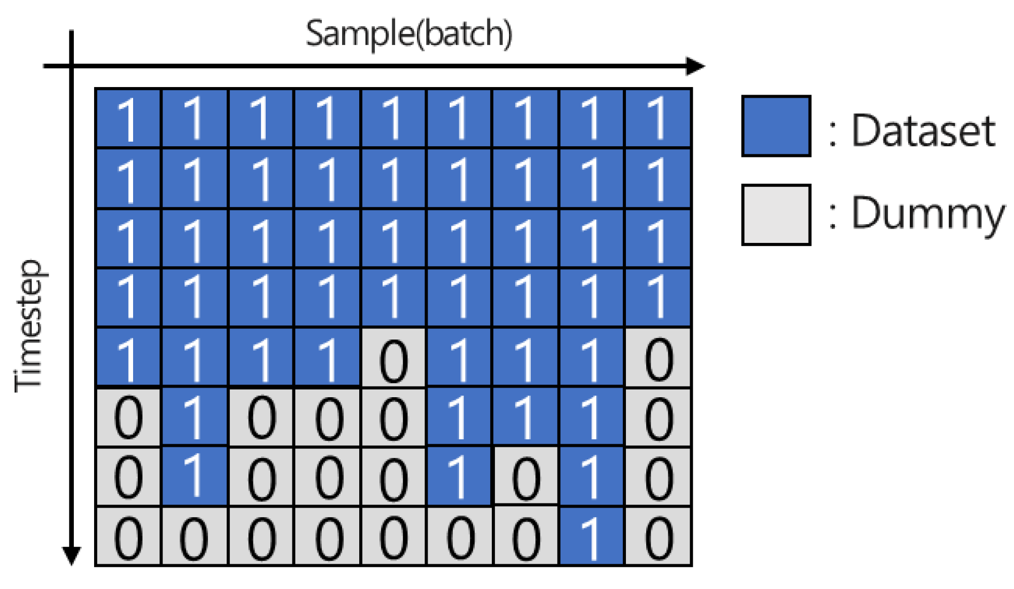
2.3. Padding and Masking Methods

Time series data have a multidimensional tensor shape that changes with time and are analyzed using specialized methods, including RNN. The preprocessing required for the RNN method involves transforming the data into a specified tensor form. Most RNN methods accept data as three-dimensional tensors of batch size, timestep, and feature dimension. In other words, all data in one mini batch must contain the same number of timesteps on the time axis and the same dimension. However, testbeds in most fields include different timesteps. For instance, in the field of natural language processing, the word count varies in different sentences. This discrepancy is compensated using several methods. Padding is one such method, wherein a dummy is attached to the dataset to fit the longest step length. Figure 2 illustrates a conceptual diagram of zero-padding. The padding method fills the amount corresponding to the insufficient step using a dummy. This method requires additional work because the dataset must be transformed during the padding process.
Another method is masking, which excludes the padded dummy in the model training process. Figure 3 depicts a conceptual diagram of the masking method. The mask value represents real and dummy data. The masking method sets the learning weight of the dummy data to zero during training. However, padding is generally set to zero as well, which poses a potential problem. When the index of the training data is expressed as zero, distinguishing between the dummy and real data becomes difficult. This is referred to as the zero-indexing problem, which can be avoided by setting a special symbol, which must be a number that does not overlap with input data.

2.4. Evaluation Index of the Carbonation Models

The performance of the carbonation model is calculated by comparing the predicted results and measured data [40]. This study used the coefficient of determination ( R 2 ) and root mean square error (RMSE) to evaluate the model. The coefficient of determination and RMSE are calculated as
R 2 = ( i = 1 N ( y i y i ¯ ) ( t i t i ¯ ) i = 1 N ( y i y i ¯ ) 2 i = 1 N ( t i t i ¯ ) 2 ) 2
R M S E = 1 N i = 1 N ( t i y i ) 2 ,
where t i and y i denote the i -th measured data and predicted results. t i ¯ and y i ¯ denote the average of measured data and predicted results, and N is number of samples.

3. Data Collection for the Case Study of Natural Carbonation

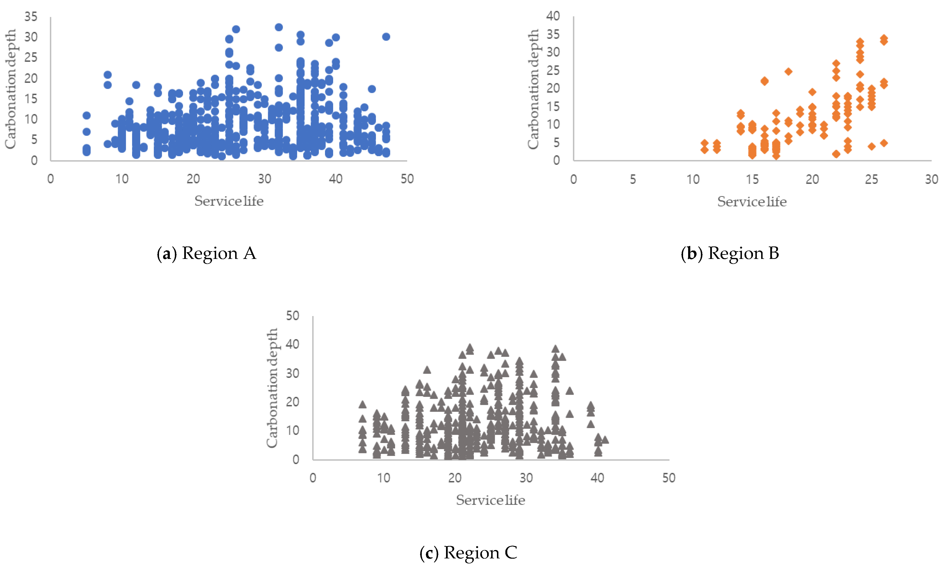
3.1. Data Description of Inspection Reports

The natural carbonation data were collected from bridge inspection reports of three regions in Korea. Typically, bridge managers conduct periodic inspections and report the test results. In this study, 242 inspection reports of RCS structures were collected from three regions. Table 1 lists the reports collected from each region. Region A was a relatively densely populated downtown area, Region B was a low-density coastal area, and Region C was an island.
The data reported for the carbonation analysis were extracted from the inspection and diagnosis reports. Each inspection report contained carbonation information; however, its format differed depending on the inspection company. In this study, carbonation data were manually extracted from inspection reports. A total of 1379 carbonation data points were extracted, which included 588 superstructures and 791 substructures. Table 2 lists the additional data collected with respect to carbonation. The construction year, inspection year, and concrete strength data directly associated with carbonation were extracted. Furthermore, we collected information related to the bridge, such as bridge length, maximum span length, width, and live load, to estimate bridge constructability. Although these variables were not theoretical factors involved in carbonation, they indirectly predicted the quality at the time of construction [36,41,42,43]. Figure 4 illustrates the carbonation depth of bridges with respect to service life. As indicated in the figure, the dispersion of the carbonation depth for service life was high, contrary to the theoretical equation. This was attributed to field bridges being exposed to conditions different from those of the laboratory environment. For instance, differences were observed in environmental conditions according to region, the quality of concrete based on the completed environment, and the history of environmental conditions as per the year of construction.

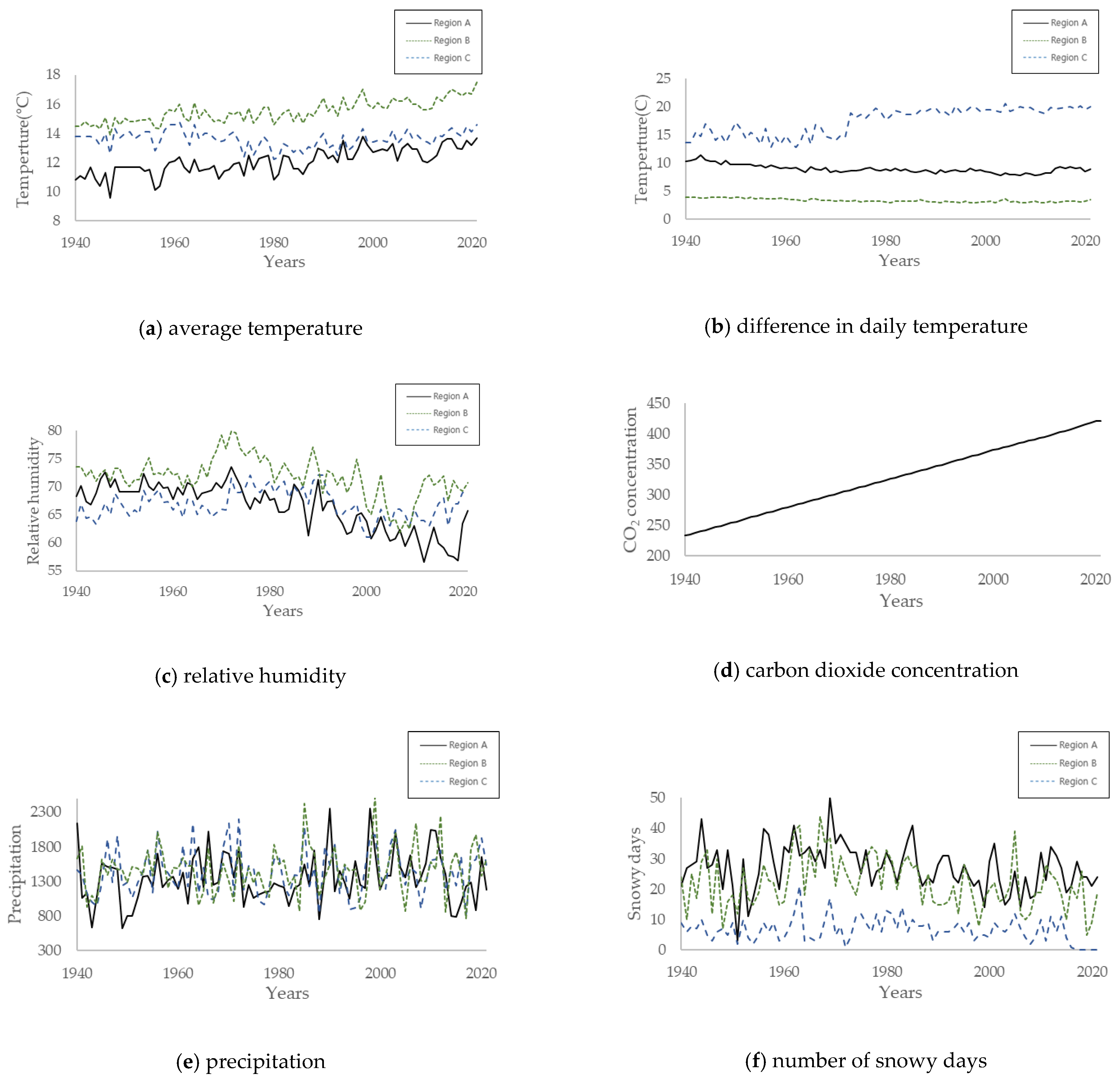
3.2. Data Description of Environmental Conditions

Regional environmental data were collected to analyze the environmental impacts of carbonation. The carbonation of concrete was affected by the mixing ratio, moisture ratio, curing period, and long-term environmental changes. In this study, regional environmental data were collected considering the long-term changes in carbonation. The environmental data were extracted from the national meteorological database of Korea [44]. The collected environmental data were organized with respect to year and region. The data were collected from 1940 to 2021, and 492 data points were collected for each region. Table 3 and Figure 5 present the environmental conditions data for each region. The collected environmental data comprised the annual average temperature, daily temperature difference, precipitation, relative humidity, carbon dioxide, and number of snowy days. The average temperature, daily temperature difference, precipitation, humidity, and carbon dioxide directly influence carbonation. The number of snowy days was included because chloride penetration by deicing agents is known to accelerate carbonation. In Korea, the carbon dioxide concentration is used as a single carbon dioxide concentration index.

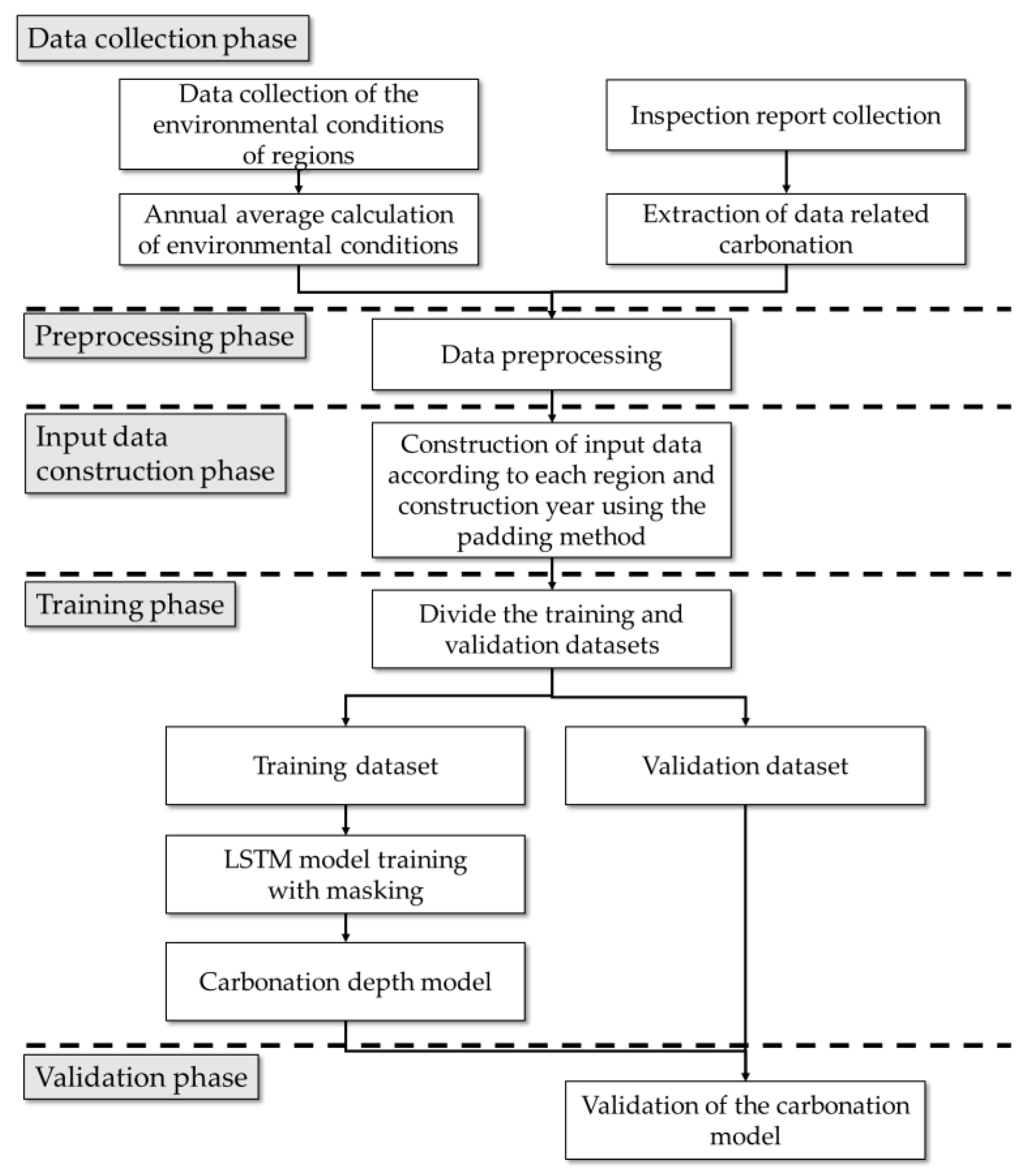
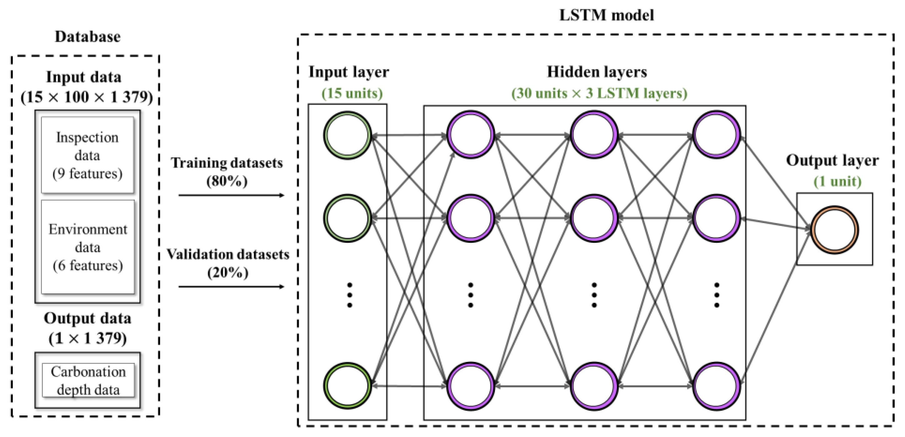
4. LSTM-Based Methodology for Generating the Carbonation Model

Figure 6 depicts the methodology developed for generating a carbonation model considering three environmental conditions. The methodology involved data collection, preprocessing, input data construction, learning, and validation phases. Initially, in the data collection phase, the data necessary for LSTM training were collected from the local environmental database and inspection reports. The number of features for the input data was 15, with 9 and 6 features extracted from the inspection and environmental data points, respectively, by year. The preprocessing phase excluded outlier data and normalized the data. To compensate for the measurement errors caused by inspectors, normalization was conducted using a robust method against outliers; the robustness was ensured because the transformation occurred such that the median was 0 and the interquartile difference range was 1.
The input data construction phase builds an input dataset to consider historical environmental data. The goal of this stage is to build time series data of environmental data according to years of service. The timestep extended up to the service life of the bridge. For instance, a bridge with a service life of 30 years was created with an input size of (15, 30), with 15 features and 30 timesteps. However, because the service life for each dataset was different, the size of the input dataset differed for each bridge. The difference in the input dataset hindered the learning of artificial intelligence, including the LSTM. In this study, a padding method was applied to correct the different timesteps according to the service life of the bridge. The timestep for the padding method was set to 100 years. For instance, a bridge with a service life of 30 years had 30 timesteps and 70 dummy timesteps.
Figure 7 illustrates the LSTM model created to predict carbonation based on the aforementioned dataset. The TensorFlow library of Python was used for model building. The LSTM layer was primarily used as the learning model; Table 4 lists all the layers of the model. The masking layer set the weights to one and zero for the existing and padded data, respectively. The weight was set to ensure that the padded dummy data in the input data were not learned. Three LSTM layers were used, and the number of LSTM input data nodes was set to 30. The activation functions of each layer were tanh, rectified linear activation unit (ReLU), and tanh. Additionally, a dropout layer of 0.5 was added to each layer to prevent overfitting. The total number of parameters in the model was 20,071.
In the learning phase, the training and validation datasets were generated by dividing the dataset. The LSTM model was trained as a carbonation model for the training dataset. The padded dummy timesteps used a masking method to ensure that the training weight was zero. This method reduced the training time by excluding dummy data and improved the reliability of the model. Finally, the trained model verified the LSTM-based carbonation model in the validation phase using the validation dataset.

5. Experimental Results

5.1. Experimental Results of the Case Study

The carbonation estimation model was trained using the input data. The model was then verified by maintaining the training and validation data ratio as 80:20. We used the random extraction method and the Adam learning method; the number of iterations was set to 100. The coefficient of determination and RMSE were selected as the performance indicators of the carbonation model. Typically, the coefficient of determination denotes the proportion of variance of the response variable, which can be explained by the applied model. In general, a coefficient of determination greater than 0.5 implies that the predictor variable can statistically predict the response variables. Table 5 and Figure 8 present the training and validation results. The learning time was 556.20 s. The hardware specifications were Intel i7-7700K CPU 4.20GHz and NVIDIA GeForce GTX 960. The coefficient of determination of the training data and the RMSE were 0.638 and 4.572, respectively. Conversely, the coefficient of determination of the verification data was 0.504, and the RMSE was 5.057. Thus, the coefficients of determination for both the training and validation datasets exceeded 0.5.
The cross-validation was conducted to check for overfitting of the proposed model. Cross-validation verifies whether a particular dataset is overfitted when the dataset has a small size. The k-fold method was used for cross-validation. The k-fold cross-validation divided the training dataset into four folds, and a total of five folds were included in the validation dataset. The distribution method was randomly selected. Figure 9 shows the results of the cross-validation. The average of the cross-validation result was 0.5028, which was slightly different from the first experimental result. This result verified that the experimental results were not overfitting for a specific dataset.

5.2. Comparison of the Proposed Methodology with Other Analysis Methods

The proposed method was compared with the existing equation-based carbonation model, wherein the model equation was developed using the same dataset as the carbonation coefficient according to Equation (1). Although previous studies have calculated the coefficient, the coefficient calculated in this study was optimized for the data to obtain the highest possible performance index. Because each region exhibited different environmental conditions, carbonation equations and the performance indicators for the three regions were generated separately. Table 6 summarizes the test results. The coefficients of determination of the equation-based carbonation model were 0.035, 0.129, and 0.016 for Regions A, B, and C, respectively; conversely, the coefficients of determination of the proposed carbonation model were 0.426, 0.542, and 0.677 for Regions A, B, and C, respectively. Therefore, the proposed model exhibited a higher performance index than that of the equation-based carbonation model.
The proposed method was compared with other regression analysis methods, including linear regression, regression trees, support vector machines, and Gaussian process regression. All regression analysis methods used the same training and validation datasets. Table 7 summarizes the performance results of the different regression analysis methods. The method with the highest coefficient of determination (0.4310) among the regression analysis methods was the rational quadratic with Gaussian process regression. The proposed carbonation model exhibited a coefficient of determination that was 16.8% higher than that of the Gaussian process regression.

6. Conclusions

Preventive maintenance of RCS bridges provides economic benefits by predicting bridge deterioration and enabling adequate performance. However, the existing carbonation models exhibit low reliability in the case of bridges exposed to varying environmental conditions as the models have been determined based on short-term period laboratory experiments. Therefore, we developed a methodology for predicting a carbonation model based on the LSTM model for RCS bridges exposed to natural environmental conditions, considering the data collected over a certain period. The proposed methodology designed an LSTM model to reflect the history of regional environmental conditions based on carbonation data. The training data for the experiment were extracted from inspection reports of bridges in Korea, and the data were divided according to region. The proposed methodology was verified by comparing it with other methodologies, such as the equation-based carbonation model and several regression analysis methods. The coefficient of determination of the result was 0.504, which was 16.8% higher than those of other regression analysis results. The average coefficient of determination of the regression model based on Fick’s second law equation was 0.06. The analysis results confirmed that the developed methodology can produce a better carbonation model than the equation-based carbonation model for the field bridges, provided sufficient data are available. Moreover, the obtained experimental results of the carbonation model were better than those reported in previous studies, thus emphasizing the need to consider long-term environmental conditions. This methodology contributes to carbonation models of field bridges adapting to environmental changes.
The proposed methodology analyzes carbonation based on field bridge inspection and climate change data. The coefficient of determination of the result was lower than that observed in the analysis performed using experimental data. This was because different managers used different equipment to measure the data during the nationwide inspections; therefore, measurement equipment and human errors were included in the inspection reports. This error caused excessive abnormalities in the collected data, which reduced the data quality and predictive performance. Additionally, the initial design mixing ratio considered in previous studies was a crucial factor affecting carbonation. However, in this study, only the information from the inspection and diagnosis reports was used for practical field applications. In the future, better results can be obtained by considering the mixing ratio during the analysis. The limitation of this study is that LSTM models can derive results that are different from scientific facts based on incomplete data. These limitations will reduce the generality and reliability of the proposed model. Therefore, future research needs a methodology to create a carbonation model by designing an artificial intelligence model based on scientific knowledge. Another limitation of this study is that the data are collected only from inspection reports. The collected data did not include concrete design information related to carbonation. Further research that builds a model including design information of concrete will have higher reliability.

Author Contributions

Data collection and preprocessing, T.H.K. and J.K.; conceptualization and methodology, T.H.K. and J.K.; validation, K.-S.J.; supervision, K.-T.P. All authors have read and agreed to the published version of the manuscript.

Funding

Research for this paper was carried out under the KICT Research Program (project no. 20220217-001, Development of DNA-based smart maintenance platform and application technologies for aging bridges) funded by the Ministry of Science and ICT.

Institutional Review Board Statement

Not applicable.

Informed Consent Statement

Not applicable.

Data Availability Statement

Not applicable.

Conflicts of Interest

The authors declare no conflict of interest.

References

  1. Miao, P.; Yokota, H.; Zhang, Y. Deterioration prediction of existing concrete bridges using a LSTM recurrent neural network. Struct. Infrastruct. Eng. 2021, 17, 1–15. [Google Scholar] [CrossRef]
  2. Rathnarajan, S.; Dhanya, B.; Pillai, R.G.; Gettu, R.; Santhanam, M. Carbonation model for concretes with fly ash, slag, and limestone calcined clay-using accelerated and five-year natural exposure data. Cement Concr. Compos. 2022, 126, 104329. [Google Scholar] [CrossRef]
  3. Kellouche, Y.; Boukhatem, B.; Ghrici, M.; Tagnit-Hamou, A. Exploring the major factors affecting fly-ash concrete carbonation using artificial neural network. Neural Comput. Appl. 2019, 31, 969–988. [Google Scholar] [CrossRef]
  4. Gattuso, J.-P.; Magnan, A.; Billé, R.; Cheung, W.W.; Howes, E.L.; Joos, F.; Allemand, D.; Bopp, L.; Cooley, S.R.; Eakin, C.M. Contrasting futures for ocean and society from different anthropogenic CO2 emissions scenarios. Science 2015, 349, aac4722. [Google Scholar] [CrossRef]
  5. Ekolu, S. A review on effects of curing, sheltering, and CO2 concentration upon natural carbonation of concrete. Construct. Build. Mater. 2016, 127, 306–320. [Google Scholar] [CrossRef]
  6. Yoon, I.-S.; Chang, C.-H. Time evolution of CO2 diffusivity of carbonated concrete. Appl. Sci. 2020, 10, 8910. [Google Scholar] [CrossRef]
  7. Kwon, S.-J.; Song, H.-W. Analysis of carbonation behavior in concrete using neural network algorithm and carbonation modeling. Cement Concr. Res. 2010, 40, 119–127. [Google Scholar] [CrossRef]
  8. Neves, A.C.; Gonzalez, I.; Leander, J.; Karoumi, R. Structural health monitoring of bridges: A model-free ANN-based approach to damage detection. J. Civil Struct. Health Monitor. 2017, 7, 689–702. [Google Scholar] [CrossRef] [Green Version]
  9. Lin, C.-J.; Wu, N.-J. An ANN model for predicting the compressive strength of concrete. Appl. Sci. 2021, 11, 3798. [Google Scholar] [CrossRef]
  10. Singh, P.; Bhardwaj, S.; Dixit, S.; Shaw, R.N.; Ghosh, A. Development of prediction models to determine compressive strength and workability of sustainable concrete with ANN. In Innovations in Electrical and Electronic Engineering; Springer: Berlin/Heidelberg, Germany, 2021; pp. 753–769. [Google Scholar]
  11. Kandiri, A.; Sartipi, F.; Kioumarsi, M. Predicting compressive strength of concrete containing recycled aggregate using modified ANN with different optimization algorithms. Appl. Sci. 2021, 11, 485. [Google Scholar] [CrossRef]
  12. Kwon, T.H.; Park, S.H.; Park, S.I.; Lee, S.-H. Building information modeling-based bridge health monitoring for anomaly detection under complex loading conditions using artificial neural networks. J. Civil Struct. Health Monit. 2021, 11, 1301–1319. [Google Scholar] [CrossRef]
  13. Cavaleri, L.; Barkhordari, M.S.; Repapis, C.C.; Armaghani, D.J.; Ulrikh, D.V.; Asteris, P.G. Convolution-based ensemble learning algorithms to estimate the bond strength of the corroded reinforced concrete. Construct. Build. Mater. 2022, 359, 129504. [Google Scholar] [CrossRef]
  14. Lu, C.; Liu, R. Predicting carbonation depth of prestressed concrete under different stress states using artificial neural network. Adv. Artif. Neural Syst. 2009, 2009, 193139. [Google Scholar] [CrossRef] [Green Version]
  15. Liu, K.; Alam, M.S.; Zhu, J.; Zheng, J.; Chi, L. Prediction of carbonation depth for recycled aggregate concrete using ANN hybridized with swarm intelligence algorithms. Construct. Build. Mater. 2021, 301, 124382. [Google Scholar] [CrossRef]
  16. Felix, E.F.; Carrazedo, R.; Possan, E. Carbonation model for fly ash concrete based on artificial neural network: Development and parametric analysis. Construct. Build. Mater. 2021, 266, 121050. [Google Scholar] [CrossRef]
  17. Felix, E.F.; Possan, E.; Carrazedo, R. Analysis of training parameters in the ANN learning process to mapping the concrete carbonation depth. J. Build. Pathol. Rehabilit. 2019, 4, 16. [Google Scholar] [CrossRef]
  18. Kellouche, Y.; Boukhatem, B.; Ghrici, M.; Rebouh, R.; Zidol, A. Neural network model for predicting the carbonation depth of slag concrete. Asian J. Civ. Eng. 2021, 22, 1401–1414. [Google Scholar] [CrossRef]
  19. Wu, N.-J. Predicting the compressive strength of concrete using an RBF-ANN model. Appl. Sci. 2021, 11, 6382. [Google Scholar] [CrossRef]
  20. Houst, Y.F.; Wittmann, F.H. Influence of porosity and water content on the diffusivity of CO2 and O2 through hydrated cement paste. Cement Concr. Res. 1994, 24, 1165–1176. [Google Scholar] [CrossRef]
  21. Sanjuán, M.Á.; Andrade, C.; Mora, P.; Zaragoza, A. Carbon dioxide uptake by cement-based materials: A Spanish case study. Appl. Sci. 2020, 10, 339. [Google Scholar] [CrossRef]
  22. Yoon, I.-S.; Çopuroğlu, O.; Park, K.-B. Effect of global climatic change on carbonation progress of concrete. Atmos. Environ. 2007, 41, 7274–7285. [Google Scholar] [CrossRef]
  23. Vu, Q.H.; Pham, G.; Chonier, A.; Brouard, E.; Rathnarajan, S.; Pillai, R.; Gettu, R.; Santhanam, M.; Aguayo, F.; Folliard, K.J. Impact of different climates on the resistance of concrete to natural carbonation. Construct. Build. Mater. 2019, 216, 450–467. [Google Scholar] [CrossRef]
  24. Sagues, A.A.; Moreno, E.; Morris, W.; Andrade, C. Carbonation in Concrete and Effect on Steel Corrosion; University of South Florida: Tampa, FL, USA, 1997. [Google Scholar]
  25. Kobayashi, K.; Uno, Y. Mechanism of carbonation of concrete. Concr. Libr. JSCE 1990, 16, 139–151. [Google Scholar]
  26. Parrott, L.J. A Review of Carbonation in Reinforced Concrete; Cement and Concrete Association: London, UK, 1987. [Google Scholar]
  27. Jiang, L.; Lin, B.; Cai, Y. A model for predicting carbonation of high-volume fly ash concrete. Cement Concr. Res. 2000, 30, 699–702. [Google Scholar] [CrossRef]
  28. Papadakis, V.G.; Vayenas, C.G.; Fardis, M.N. Experimental investigation and mathematical modeling of the concrete carbonation problem. Chem. Eng. Sci. 1991, 46, 1333–1338. [Google Scholar] [CrossRef]
  29. Khunthongkeaw, J.; Tangtermsirikul, S.; Leelawat, T. A study on carbonation depth prediction for fly ash concrete. Construct. Build. Mater. 2006, 20, 744–753. [Google Scholar] [CrossRef]
  30. Londhe, S.; Kulkarni, P.; Dixit, P.; Silva, A.; Neves, R.; de Brito, J. Tree based approaches for predicting concrete carbonation coefficient. Appl. Sci. 2022, 12, 3874. [Google Scholar] [CrossRef]
  31. Niu, D.; Dong, Z.; Pu, J. Random model of predicting the carbonated concrete depth. Ind. Construct. 1999, 29, 41–45. [Google Scholar]
  32. Chang, C.-F.; Chen, J.-W. The experimental investigation of concrete carbonation depth. Cement Concr. Res. 2006, 36, 1760–1767. [Google Scholar] [CrossRef]
  33. Sisomphon, K.; Franke, L. Carbonation rates of concretes containing high volume of pozzolanic materials. Cement Concr. Res. 2007, 37, 1647–1653. [Google Scholar] [CrossRef]
  34. Dhir, R.; Hewlett, P.; Chan, Y. Near-surface characteristics of concrete: Prediction of carbonation resistance. Mag. Concr. Res. 1989, 41, 137–143. [Google Scholar] [CrossRef]
  35. Roy, S.; Beng, P.K.; Northwood, D. The carbonation of concrete structures in the tropical environment of Singapore and a comparison with published data for temperate climates. Mag. Concr. Res. 1996, 48, 293–300. [Google Scholar] [CrossRef]
  36. Guiglia, M.; Taliano, M. Comparison of carbonation depths measured on in-field exposed existing RC structures with predictions made using fib-Model Code 2010. Cement Concr. Compos. 2013, 38, 92–108. [Google Scholar] [CrossRef]
  37. Walraven, J.C. Model Code 2010-Final Draft: Volume 1; FIB—Fédération Internationale du Béton: Lausanne, Switzerland, 2012; Volume 65. [Google Scholar]
  38. Mikolov, T.; Karafiát, M.; Burget, L.; Cernocký, J.; Khudanpur, S. Recurrent neural network based language model. In Proceedings of the Interspeech, Chiba, Japan, 26–30 September 2010; pp. 1045–1048. [Google Scholar]
  39. Hochreiter, S.; Schmidhuber, J. Long short-term memory. Neural Comput. 1997, 9, 1735–1780. [Google Scholar] [CrossRef] [PubMed]
  40. Dou, Z.; Sun, Y.; Zhang, Y.; Wang, T.; Wu, C.; Fan, S. Regional manufacturing industry demand forecasting: A deep learning approach. Appl. Sci. 2021, 11, 6199. [Google Scholar] [CrossRef]
  41. Song, L.; Liu, J.; Cui, C.; Yu, Z.; Fan, Z.; Hou, J. Carbonation process of reinforced concrete beams under the combined effects of fatigue damage and environmental factors. Appl. Sci. 2020, 10, 3981. [Google Scholar] [CrossRef]
  42. Shi, X.; Yao, Y.; Wang, L.; Zhang, C.; Ahmad, I. A modified numerical model for predicting carbonation depth of concrete with stress damage. Construct. Build. Mater. 2021, 304, 124389. [Google Scholar] [CrossRef]
  43. Duan, K.; Cao, S. Data-driven parameter selection and modeling for concrete carbonation. Materials 2022, 15, 3351. [Google Scholar] [CrossRef]
  44. Korea Meteorological Administration. National Climate Data Center. Available online: https://data.kma.go.kr/resources/html/en/ncdci.html (accessed on 16 November 2022).
Figure 1. Conceptual structure of the long short-term memory (LSTM).
Applsci 12 12470 g001
Figure 2. Conceptual structure of the padding method.
Applsci 12 12470 g002
Figure 3. Example of weight matrix of the masking method.
Applsci 12 12470 g003
Figure 4. Carbonation depth according to regions: (a) Region A; (b) Region B; and (c) Region C.
Applsci 12 12470 g004
Figure 5. History of environmental conditions according to regions: (a) average temperature; (b) difference in daily temperature; (c) relative humidity; (d) carbon dioxide concentration; (e) precipitation; and (f) number of snowy days.
Applsci 12 12470 g005
Figure 6. Methodology for generating a carbonation model for actual bridges.
Applsci 12 12470 g006
Figure 7. Proposed LSTM model for generating the carbonation models.
Applsci 12 12470 g007
Figure 8. Carbonation prediction results of the LSTM model for the (a) training and (b) validation datasets.
Applsci 12 12470 g008
Figure 9. The k-fold cross-validation test results of the proposed model.
Applsci 12 12470 g009
Table 1. Characteristics and number of inspection reports collected from different areas.
RegionNumber of ReportsCharacteristics Area   ( k m 2 )
Region A137High-densely
downtown area
600
Region B22Low-density
coastal area
1850
Region C166Low-density
island
10,550
Table 2. Data extracted from the inspection reports.
ClassificationFactorsAverageMinMax
Carbonation-related factorsService life24.79547
Year of construction1989.6519692010
Concrete strength23.421835
Indirect factorsLength83.195.2261
Maximum span length17.70555
Width18.87461.48
Height6.67229.5
Loading condition for design22.0813.524
Element position
(superstructure and
substructure)
-0
(superstructure)
1
(substructure)
CarbonationCarbonation depth10.510240
Table 3. Environmental conditions data for each region.
ClassificationFactorsRegionAverageMinMax
Temperature (°C)Average temperatureA12.19.613.8
B13.612.214.8
C15.513.917.5
Daily temperature differenceA9.07.811.4
B17.512.820.5
C3.42.94
HumidityRelative humidityA66.456.673.6
B66.86172
C71.761.879.8
Carbon dioxideCarbon dioxide concentrationA327.5233.5421.4
B
C
PrecipitationPrecipitationA1344.9623.52355.5
B1431.7819.32195.5
C1465.9773.32526
Chloride penetrationNumber of snowy daysA27.1350
B6.6021
C22.0544
Table 4. Long short-term memory (LSTM) model layer for the carbonation model.
NumberLayer NameHidden UnitActivation FunctionNumber of Parameters
1LSTM30tanh5400
-Dropout--
2LSTM30ReLU7320
-Dropout--
3LSTM30tanh7320
-Dropout--
4Dense1Linear31
Table 5. Performance indicators of the carbonation model.
Performance IndicatorValue
Training dataset R 2 0.638
Training dataset RMSE4.572
Validation dataset R 2 0.504
Validation dataset RMSE5.057
Table 6. LSTM model layer for the carbonation model.
RegionMethodology R 2 RMSE
AProposed model0.4264.970
Fick’s second law equation0.0356.411
BProposed model0.5425.556
Fick’s second law equation0.1297.377
CProposed model0.6775.132
Fick’s second law equation0.0168.793
Table 7. Carbonation model prediction results of other regression methods.
Regression Analysis MethodValidation Dataset
R 2 RMSE
Linear regressionLinear0.13227.260
Interaction linear0.22036.898
Robust linear0.13027.373
Stepwise linear0.21026.928
TreeComplex tree0.38776.157
Medium tree0.33676.363
Simple tree0.21616.932
Support vector machineLinear0.12597.537
Quadratic0.24576.868
Cubic0.22297.182
Fine Gaussian0.37566.220
Gaussian process regressionSquared exponential0.42205.964
Matern 5/20.42355.955
Rational quadratic0.43105.910
Publisher’s Note: MDPI stays neutral with regard to jurisdictional claims in published maps and institutional affiliations.

