Abstract
The Intra-Voxel Incoherent Motion (IVIM) model allows to estimate water diffusion and perfusion-related coefficients in biological tissues using diffusion weighted MR images. Among the available approaches to fit the IVIM bi-exponential decay, a segmented Bayesian algorithm with a Conditional Auto-Regressive (CAR) prior spatial regularization has been recently proposed to produce more reliable coefficient estimation. However, the CAR spatial regularization can generate inaccurate coefficient estimation, especially at the interfaces between different tissues. To overcome this problem, the segmented CAR model was coupled in this work with a k-means clustering approach, to separate different tissues and exclude voxels from other regions in the CAR prior specification. The proposed approach was compared with the original Bayesian CAR method without clustering and with a state-of-the-art Bayesian approach without CAR. The approaches were tested and compared on simulated images by calculating the estimation error and the coefficient of variation (). Furthermore, the proposed method was applied to some illustrative real images of oncologic patients. On simulated images, the proposed innovation reduced the average error of 47%, 21% and 58% for D, f and , respectively, compared to the state-of-the-art Bayesian approach, and of 48% and 34% for D and f, respectively, compared to the original CAR, while it achieved the same error for . The clustering approach was also able to consistently reduce the for each coefficient. On real images, the novel approach did not alter the IVIM maps obtained by the original CAR method, with the advantage of reducing their typical blotchy appearance at the boundaries. The proposed approach represents a valuable improvement over the state-of-the-art Bayesian CAR method and provides more reliable IVIM coefficient estimation, and is less sensitive to bias and inconsistency at tissue/tissue and tissue/background interfaces.
1. Introduction
Intravoxel Incoherent Motion (IVIM) Magnetic Resonance Imaging (MRI) is a type of Diffusion-Weighted MRI (DW-MRI) acquisition, firstly proposed by Le Bihan et al. [1], for estimating diffusion and perfusion tissue properties. In the IVIM mathematical representation, a bi-exponential function of the diffusion signal decay at different b-values is used to simultaneously characterize tissue diffusivity and perfusion within capillaries. Specifically, the IVIM model allows us to estimate the diffusion (D) and pseudo-diffusion coefficients (), along with the perfusion volume fraction (f) within the tissue.
IVIM has gained particular interest in oncologic applications, especially in the last decade, thanks to the advancements in MRI hardware, pulse design and post-processing methods [2]. In fact, recent works have proposed the adoption of the IVIM model to improve tumor diagnosis [3], prognosis [4] and response to treatment [5]. Furthermore, IVIM has also been used to characterize radiation-induced modifications in normal tissues after radiotherapy [6]. Nevertheless, the use of the IVIM technique is not confined to oncology, but it has significant potential in clinical and preclinical applications for neurological diseases [7] and other physio-pathological conditions [8,9].
However, IVIM coefficient estimation presents several issues related to the presence of noise over the image, the correct model identification and the amount of tissue perfusion [10]. Currently, the most popular techniques to fit IVIM data are (i) the non-linear least-square (LSQ) fitting, based on the Levenberg–Marquardt algorithm [11], and (ii) the Bayesian approach, which provides the posterior probability densities of the coefficients based on prior knowledge [12].
The Bayesian method showed superior performance in reducing errors and variability [12], and also allowed the inclusion of a spatial dependence between voxels, to obtain more regular maps. This is the case of the spatial homogeneity prior [13] and the Conditional Auto-Regressive (CAR) prior specification, which takes into account information from the neighbor voxels [14,15]. In particular, it was reported that the CAR specification on a segmented Bayesian method improved the estimation accuracy compared to both LSQ and traditional Bayes approaches, especially for [15]; however, a limitation of the CAR method lies in the choice of the neighborhood, as it attributes the same weight to all surrounding voxels without considering the continuity of the structure. This leads to a slight decrease in the quality of the IVIM coefficient maps, especially at the tissue/tissue and tissue/background interfaces, characterized by a blotchy appearance.
The goal of this work was to overcome this limitation by coupling the CAR prior with a k-means clustering approach, which distinguishes the different structures based on the diffusion signal decay along the b-values, and uses this information to set different weights to the contributions of the different neighbor voxels. This technological improvement was aimed to obtain more regular and reliable IVIM parametric maps. The voxel-based estimation of IVIM coefficients can be used in the clinical practice for the characterization of microstructural properties of diffusion and perfusion within subregions of organs/structures. This information can be useful, for example, to define prediction models for treatment response in oncology or to assess changes occurring in physiological and pathological conditions in different applications; therefore, the availability of high quality and accurate maps represents a paramount condition in clinical practice and improved quality maps may have, prospectively, an impact on the quality of care
The proposed method was compared to the original CAR approach and a state-of-the-art Bayesian algorithm in terms of accuracy and map homogeneity. First, it was applied to a set of simulated phantoms for which the true value of the IVIM coefficients was known. Then, it was applied to some illustrative real images of oncologic patients, to evaluate the estimated maps in a real clinical scenario.
2. Materials and Methods
2.1. IVIM Fitting Procedure
The decay of the signal intensity in function of b is described in any voxel by a bi-exponential function, according to the IVIM model [16]:
where , and are the diffusion coefficient, the pseudo-diffusion coefficient and the perfusion volume fraction in voxel , respectively. The goal of the fitting is to estimate these three coefficients in each voxel of a region of interest, based on a set of signal intensity observations in an image domain at different b-values.
2.1.1. Clustering Approach
In the proposed approach, a clustering technique is employed to determine the cluster associated with each voxel . Then, a Bayesian CAR fitting is performed, where the CAR prior specification depends on the clustering solution .
The k-means clustering approach is chosen for its simplicity and low computational cost, and because it is one of the most widely adopted clustering methods for medical image segmentation. It is employed by assuming as the distance between any pair of voxels the distance between the vectors of their signal intensities over . Moreover, the number of clusters is set equal to 9, which is reasonable from a theoretical viewpoint, as it represents the combinations of two levels (low or high) for the three coefficients to be estimated plus an additional case for the background (); therefore, it gives enough flexibility to recognize these macroscopically different behaviors.
The results of the clustering procedure is the cluster of each voxel , where all voxels belonging to the same cluster have the same value.
The clustering was implemented in MATLAB (R2020a, The MathWorks Inc., Natick, MA, USA), with the function “kmeans”, imposing 50 replicates with alternative initial cluster centroid positions.
2.1.2. Bayesian CAR Fitting
This fitting procedure is taken from [15], where a segmented approach was considered by dividing the estimation procedure in two steps.
In the first step, the coefficients and , where denotes an intermediate estimation of f, are estimated with the observations at and , with s/mm. A simplified version of the IVIM model is used, which only includes the second exponential decay:
In the second step, the coefficients and are estimated using all observations . The complete IVIM model (1) is used while fixing coefficients to the values estimated in the first step (the expected value of the marginal posterior density).
To perform the Bayesian fitting, (2) and (1) are processed to derive the likelihood function for the first and second step, respectively, as reported in the Supplementary Materials. This likelihood also depends on an additional parameter to be estimated, i.e., the standard deviation of the conditioned densities that determine it.
Then, a prior density for the unknown parameter is assumed. A priori independence between , each and each is assumed for the first step, and between , each and each for the second step.
Separately for each (where generically denotes each coefficient D, , f or ), a CAR specification is included in the prior by considering the intrinsic CAR formulation of Leroux et al. [17]. More specifically, the following distribution for a coefficient in a voxel given the values in the other voxels is taken:
where , and denotes the spatial neighborhood matrix.
We assume a dependency () only for the voxels bordering on . Their values are assigned based on the clustering solution . In particular, if the bordering voxel belongs to the same cluster of voxel (i.e., ), or if the bordering voxel does not belong to the same cluster of voxel (i.e., ); therefore:
In addition, to smooth the autoregressive component, the actual prior density of each consists of a mixture model with two components: the above conditional autoregressive specification (3) and a truncated Gaussian marginal density , where and denote the minimum and maximum admissible values, respectively. Therefore, the overall prior for each coefficient is a mixture between (3) and the Gaussian component, with weight 0.75 for the CAR specification (3) and weight 0.25 for the Gaussian component. The hyperparameters are detailed in Section 1 of the Supplementary Materials.
Finally, the prior of the standard deviation parameter is an independent Gamma density to respect its positivity, i.e., . The scale parameter is set equal to 1 to give a large density, while the mean value is set to half of the average over .
The approach was coded in R with package STAN [18], which directly provides the posterior marginal densities of each parameter.
The whole procedure is sketched in Figure 1. The clustering processes the signal intensity to determine the clusters , which are used in the next steps to estimate the weights in the CAR prior specification. The input of both steps of the Bayesian CAR fitting are thus the output of the clustering, together with the signal intensity itself. The first step produces the coefficients and , which are passed as input to the second step. The second step produces the coefficients and .
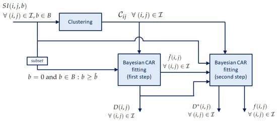
Figure 1.
Block diagram of the IVIM fitting procedure with clustering.
2.2. Evaluation
2.2.1. Simulated Data
We applied our method on simulated DW-MRI signals with different noise levels to test the performance of the proposed approach. To increase the complexity of the simulated dataset, a Shepp–Logan phantom (matrix size ) with three regions of interest (ROIs) along with background noise was used as a template for our simulations. Each ROI was characterized by an IVIM coefficient triplet randomly generated from uniform distributions and a specific intensity at . More specifically, D was sampled in the interval , in the interval and f in the interval , which include typical values of tumor and normal tissues. Images were generated using (1) for two different b-values sets, i.e., and .
Rician noise was finally added to create the final DW-MRI images with different Signal-to-Noise Ratios (s), equal to 10, 25, 50, 100, 150 and 200. Five numerical phantoms for each combination of b-value set and were generated, for a total of 60 simulated cases.
Numerical phantoms were generated using a MATLAB custom-made script.
2.2.2. Real Data
DW-MRI images of five Head-and-Neck (HN) patients affected by oropharyngeal tumor (three males and two females) and four pelvic patients affected by rectal tumor (two males and two females) were considered as examples of IVIM acquisitions for tumor diagnosis. They were collected from retrospective studies approved by the local ethics committee and already published in previous works [14,15,19].
DW-MRI images were acquired using a system (Optima MR 450w, GE Healthcare, Milwaukee, WI, USA) and obtained by single-shot spin-echo echo-planar imaging with: acquisition matrix equal to ; in-plane resolution equal to 1.094 × 1.094 mm; TR/TE equal to 4500 ms/72 ms for HN and 3500 ms/77 ms for pelvis; slice thickness equal to 4 mm for HN and 5 mm for pelvis; same b-values as in the simulated images. The estimated average of the acquired images was equal to 80 and 50 for the HN and pelvis, respectively; in this way, we were able to test the performance of the methods at different values also in the real setting.
Three different tissues were considered in the two datasets: masticatory muscle, parotid gland and tumor for HN; internal obturator muscle, prostate and rectal tumor for pelvis. An average of 4–5 slices containing the three structures of interest were selected for each patient, excluding basal and apical slices to avoid partial volume effects, for a total of 39 two-dimensional images (21 for HN and 18 for pelvis). In the two female pelvic patients, one structure (the prostate) was not considered.
2.2.3. Comparison with State-of-the-Art Methods
Maps estimated with the proposed approach were compared to the CAR approach without clustering, already published in [15], and to a state-of-the-art Bayesian approach without spatial regularization [20]. As for the CAR without clustering, it follows the description reported in Section 2.1.2 but neglecting the clustering solution. Indeed, the weights of the CAR prior specification are set equal to 1 for all voxels bordering on , and 0 for the others:
As for the standard Bayesian approach, we adopted the implementation provided by Gustafsson et al. [20], considering the default priors and the hyperparameters proposed by the authors. The IVIM signal was fitted using the bi-exponential decay in (1) and considering the whole set of b-values. The three IVIM coefficients and each signal at were estimated under the following priors [20]: a uniform prior for f and each ; a lognormal prior for D and . Moreover, all prior distributions were truncated to the following intervals: for D; for ; for f; for being the simulated images in this range. The parameter estimates were given in terms of the mean value from the respective marginalized posterior distribution.
Following the procedures already adopted in previous works [10,14,15], the accuracy of each method on simulated images was evaluated in a voxel in terms of the error with respect to the true value:
where is the estimated value of the coefficient and the corresponding true value. The median of the errors over the voxels of a ROI was finally calculated for each coefficient.
Moreover, the noisiness of the map was evaluated in terms of the coefficient of variation (), calculated as the ratio between the standard deviation and the mean value of the estimated coefficients in a ROI with constant :
The average value of the over the ROIs was then considered.
A statistical analysis was performed to evaluate the differences among the three approaches. A Kruskal–Wallis test was applied to and estimated with the three methods for each value, in order to identify significant differences among groups. For those groups presenting significant differences, a Tuckey post hoc test was next performed to determine which couples were significant. Significance was set to , and Bonferroni correction for multiple comparisons was applied.
IVIM maps estimated on real cases were qualitatively evaluated and mean values of IVIM coefficients were calculated within each structure.
3. Results
3.1. Simulated Data
The qualitative comparison of the estimated maps among the three different methods revealed that the CAR clustering approach was able to improve their quality with respect to the Bayesian CAR method without clustering and the state-of-the-art Bayesian approach without CAR (Figure 2).
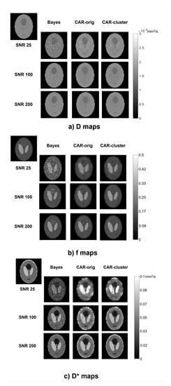
Figure 2.
Parametric maps of D (a), f (b) and (c), estimated from a simulated image using the three methods (columns) at different values (rows). The true maps are also reported in the top left corner.
The Bayesian estimation without CAR generated maps with high contrast between different structures, but maintained a certain level of noise throughout the image, especially at low values. On the contrary, the CAR approach without clustering was able to generate homogeneous values within the ROIs, but at the same time it lost the boundaries between the regions and introduced blurring and blotchy artifacts, especially at low values and for . Instead, the proposed approach with clustering better highlighted the contrast between structures at the interfaces, and preserved a high homogeneity within the regions; therefore, it retained the advantages of both other methods.
The error maps reported in Figure 3 make it evident that the high errors at the boundaries of the structures in the CAR maps were almost completely eliminated with the clustering approach, especially for high values. In addition, it can be seen from the maps that, in both CAR approaches, values were highly dependent on the IVIM coefficient values (i.e., some specific triplets were more difficult to be estimated), whilst the Bayesian method without CAR seemed less dependent. In particular, it showed for D the same error level throughout the whole image.
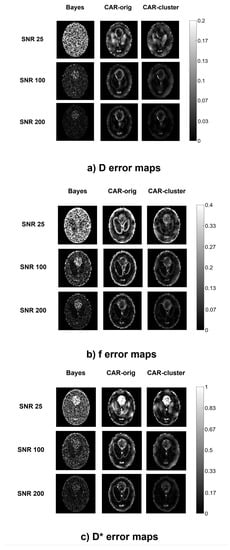
Figure 3.
Error maps of D (a), f (b), (c), computed from a simulated image using the three methods (columns) at different values (rows).
Figure 4 shows for each the barplots of and averaged on the simulated images with the corresponding significance, while the detailed results for each specific simulation are reported in the Supplementary Materials Tables S1–S4. Similar trends of and can be observed for the three methods, with higher values at low that decrease at high , as expected. The accuracy was generally higher under the proposed approach with clustering as regards the estimation of D and f: on D presented an averaged reduction of 46% compared to the other approaches, which was significant for , and ; on f reduced of 21% compared to the Bayesian approach without CAR and of 34% compared to the CAR without clustering, although this was not statistically significant. As for , similar errors were obtained for both CAR approaches, lower than for Bayesian approach without CAR (non-significant reduction of about 58%). was always the lowest for the proposed approach with the clustering, for each IVIM coefficient and value. Specifically, the introduction of clustering reduced the of about 25–55% compared to traditional Bayes, and of about 30% compared to the original CAR approach. Furthermore, for maps at low , the two CAR approaches presented similar s, and a significant reduction was found only between the original Bayesian approach without CAR and the CAR with clustering. On the contrary, for high the original CAR without clustering and the traditional Bayesian approach were almost comparable, whilst the introduction of clustering significantly reduced the compared to both of them; therefore, the CAR with clustering was able to improve not only the quality of the maps, especially on the boundaries of the structures, but also the estimation of the IVIM coefficients with respect to the other methods.
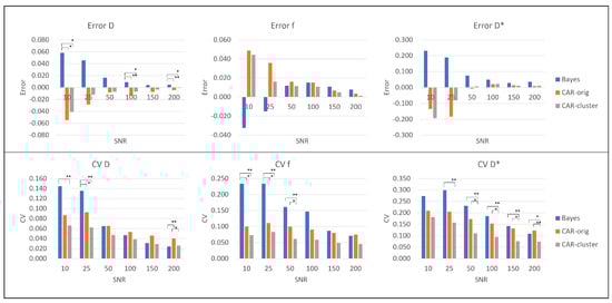
Figure 4.
Error (first row) and (second row) for the simulated images: values for D (first column), f (second column) and (third column). Significant differences are indicated by * (p < 0.05) and ** (p < 0.001).
3.2. Real Data
The IVIM maps estimated on an illustrative slice of a HN and a pelvic patient using the three different methods are shown in Figure 5 and Figure 6, respectively. The maps estimated with the clustering were almost similar to those estimated with the CAR method without clustering. The most relevant differences lie in the more defined boundaries of contrasted structures (e.g., the external boundary in the HN case, and the bladder wall and cortical bone of the femoral head in the pelvic case) and in the reduced blurred effects.
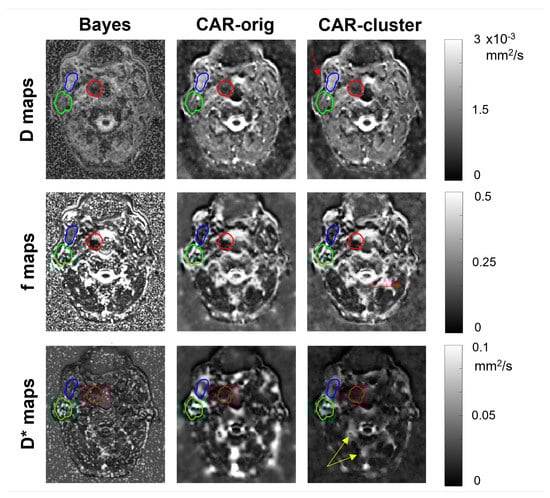
Figure 5.
Parametric maps of D (first row), f (second row) and (third row), estimated from a selected slice of a HN patient using the three methods (columns). The tumor, the parotid gland and the masticatory muscle are delineated in red, green and blue, respectively. Red arrows indicate improvement in boundary definition, yellow arrows indicate reduced blurred effects.
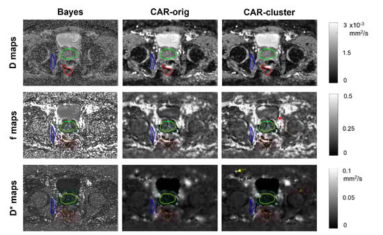
Figure 6.
Parametric maps of D (first row), f (second row) and (third row), estimated from a selected slice of a pelvic patient using the three methods (columns). The tumor, the prostate and the internal obturator muscle are delineated in red, green and blue, respectively. Red arrows indicate improvement in boundary definition, yellow arrows indicate reduced blurred effects.
D, f and values estimated by the three methods and averaged over the HN and the pelvic patients are reported in Table 1. As expected, the variations between the original CAR and that with clustering were limited, whilst the Bayesian approach without clustering showed different values, especially for .

Table 1.
Values of D, f and estimated from the real images in each structure of interest by the three methods, reported in terms of mean and standard deviation over the subjects.
4. Discussion and Conclusions
In this work, we have proposed an improvement to the Bayesian CAR fitting of the IVIM model [15] by embedding a k-means clustering procedure to specify the weights in the CAR prior specification. The aim was to improve the estimation of the parametric maps for the IVIM coefficients. In fact, in the previous work [15], it was highlighted that the main limitation of the CAR approach was in the way the neighbor voxels were considered in the fitting procedure, since all the eight surrounding voxels were included with the same weight, thus neglecting the heterogeneity of the surrounding tissues.
The simplest solution to this issue from a theoretical point of view is to also estimate all weights of all voxels by means of the Bayesian approach; however, this approach proved to be ineffective due to the huge number of parameters to be estimated and the too high computational effort. In fact, this is not pursued in the literature, while only examples are available in other applications in which the weight of the CAR component is tuned as a whole without distinguishing the contributions of the specific elements in the neighborhood [21].
To overcome this issue, the weights have been provided by embedding a k-means clustering approach in the procedure, based on a distance function that considers the whole set of images at different b-values. This allows us to group the voxels with similar exponential decay and to give them higher weights. It is worth noticing that a simpler clustering approach based only on the anatomical information brought by the image at was not sufficient to reduce the blurring effects, since it is not able to capture tissue-specific differences in the diffusion signal decay. This also shows that a manual clustering is rather impossible for this problem, as it should require to analyze “as a whole” the entire set of images at different b-values, which is a very difficult task for a human operator. In fact, no work in the literature considers this manual procedure on diffusion signal dynamic.
As the k-means requires to enter the number of clusters as input, we performed a preliminary sensitivity analysis on a subset of data. We found that the clusters usually remain quite invariant within the region of interest, while additional clusters are identified in the background. In the real images, we also found that for different clusters are assigned to voxels in regions disjoint from each other, which belong to the same cluster for , while the shape of the connected regions in the clusters does not change. Since the CAR prior is not affected by this difference, we have chosen to limit the number of clusters to 9. On the contrary, on real images, a lower number of clusters may not be able to satisfactorily reduce the blotchy effect produced by the original CAR approach.
Results on simulated data have confirmed that the improved approached based on the clustering is able to face the CAR limitations, showing less noisy IVIM maps and sharper boundaries definition at the interfaces between structures, associated with reduced errors at the boundaries. In addition, comparable results were obtained from simulations generated at different b-values, considering both HN and pelvic setups.
The application to some illustrative real oncologic cases has highlighted that the introduction of the clustering did not alter the IVIM maps estimation obtained by the original CAR method, with the advantage of reducing the typical blotchy appearance at the boundaries, which usually affects the CAR approach, especially at low s and for the estimation of .
The proposed method was able to generate IVIM maps with lower errors and higher quality compared to the original CAR and also to the standard Bayesian approach. Compared to other approaches that adopted a spatial homogeneity prior [13], the results with the CAR approach were similar in terms of map quality and accuracy, as already discussed in [15]. Even if a fair direct quantitative comparison between these works is not possible, it seems that the introduction of clusters in the CAR prior may give more regularized maps than those presented in [13], at least for simulated images.
Recently, approaches based on deep neural networks (DNNs) have been introduced to estimate IVIM parametric maps [22,23,24]. In these works, it was reported a higher quality of the maps compared to those estimated using traditional least squared and Bayesian methods. Specifically, Kaandorp et al. [23] stated that an optimized DNN can improve IVIM estimation for tissues with low perfusion and on images with low , and generate less noisy maps with more robust estimation over neighbor voxels. In our work, we have not compared our method with DNN-based approaches; however, we are confident that our results are in line with those reported in [22,23,24]. In fact, thanks to the introduction of a spatial dependency through the CAR prior specification, the continuity between adjacent voxels that share the same diffusion and perfusion properties was guaranteed. Furthermore, our estimation accuracy was high even at very low , probably comparable with that obtained by DNNs (a direct comparison is not possible, as different setups and simulations were adopted).
The major limitation of the proposed method is that, although the clustering approach is computationally efficient, the overall approach suffers from high computational load and time because of the Bayesian estimation. Compared to the previously proposed CAR [15], the computational time is not increased by the presence of different weights, but it is anyway high. A further limitation lies in the reduced number of b-values samplings that were considered in the tests. Though, in our results, the performance improvement seemed independent of the b-values, a future work might be focused on evaluating the impact of b-values choice on the performance. Finally, the proposed method was evaluated on a limited number of real cases, looking only at two body districts and at a reduced number of structures; therefore, its application to a larger dataset would allow a better evaluation of its impact from a clinical perspective.
In conclusion, this paper described a novel IVIM fitting approach, based on embedding the k-means clustering approach in the Bayesian CAR method. The proposed method provided more accurate and robust parametric maps with respect to traditional voxelwise approaches, even at the tissue/tissue and tissue/background interfaces. The tool was proven to be effective in both simulated and real cases, and represents a valuable alternative to fit the bi-exponential IVIM model in biomedical applications.
Supplementary Materials
The following supporting information can be downloaded at: https://www.mdpi.com/article/10.3390/app12041907/s1, Table S1: Median error for each simulated image at SNR10, SNR25 and SNR50 using the three different methods. HN: Head-and-Neck simulations; P: pelvis simulations; Table S2: Median error for each simulated image at SNR100, SNR150 and SNR200 using the three different methods. HN: Head-and-Neck simulations; P: pelvis simulations; Table S3: for each simulated image at SNR10, SNR25 and SNR50 using the three different methods. HN: Head-and-Neck simulations; P: pelvis simulations; Table S4: for each simulated image at SNR100, SNR150 and SNR 200 using the three different methods. HN: Head-and-Neck simulations; P: pelvis simulations.
Author Contributions
Conceptualization, E.S., A.M., G.R. and E.L.; methodology, E.S., A.M. and E.L.; formal analysis, E.S. and E.L.; data curation, E.S.; writing—original draft preparation, E.S. and E.L.; writing—review and editing, E.S., A.M., G.R. and E.L.; supervision, G.R. All authors have read and agreed to the published version of the manuscript.
Funding
This research received no external funding.
Institutional Review Board Statement
The study was conducted according to the guidelines of the Declaration of Helsinki and approved by the Institutional Ethics Committee of Regina Elena Scientific Institute, Rome, Italy (RS 266/12).
Informed Consent Statement
Informed consent was obtained from all subjects involved in the study.
Data Availability Statement
Part of the data presented in this study are openly available in Zenodo at https://doi.org/10.5281/zenodo.5924820, accessed on 9 February 2022. Restrictions apply to the availability of the clinical datasets used in this paper. Data were obtained from Regina Elena Scientific Institute, Rome, Italy and are available from the corresponding author with the permission of Regina Elena Scientific Institute.
Acknowledgments
The authors acknowledge Simona Marzi and Antonello Vidiri from the Regina Elena National Cancer Institute, Rome, Italy, for having provided the images of real cases, already used in previous studies. The authors also acknowledge Mattia Begnis and Yasmine Chaar, for their support in the implementation of the clustering approach.
Conflicts of Interest
The authors declare no conflict of interest.
References
- Le Bihan, D.; Breton, E.; Lallemand, D.; Grenier, P.; Cabanis, E.; Laval-Jeantet, M. MR Imaging of Intravoxel Incoherent Motions: Application to Diffusion and Perfusion in Neurologic Disorders. Radiology 1986, 161, 401–407. [Google Scholar] [CrossRef] [PubMed]
- Federau, C. Intravoxel Incoherent Motion MRI as a Means to Measure In Vivo Perfusion: A Review of the Evidence. NMR Biomed. 2017, 30, e3780. [Google Scholar] [CrossRef] [PubMed]
- Ding, Y.; Tan, Q.; Mao, W.; Dai, C.; Hu, X.; Hou, J.; Zeng, M.; Zhou, J. Differentiating between Malignant and Benign Renal Tumors: Do IVIM and Diffusion Kurtosis Imaging Perform Better than DWI? Eur. Radiol. 2019, 29, 6930–6939. [Google Scholar] [CrossRef] [PubMed]
- Noij, D.P.; Martens, R.M.; Marcus, J.T.; de Bree, R.; Leemans, C.R.; Castelijns, J.A.; de Jong, M.C.; de Graaf, P. Intravoxel Incoherent Motion Magnetic Resonance Imaging in Head and Neck Cancer: A Systematic Review of the Diagnostic and Prognostic Value. Oral Oncol. 2017, 68, 81–91. [Google Scholar] [CrossRef] [PubMed]
- Nougaret, S.; Vargas, H.A.; Lakhman, Y.; Sudre, R.; Do, R.K.; Bibeau, F.; Azria, D.; Assenat, E.; Molinari, N.; Pierredon, M.A.; et al. Intravoxel Incoherent Motion–Derived Histogram Metrics for Assessment of Response after Combined Chemotherapy and Radiation Therapy in Rectal Cancer: Initial Experience and Comparison between Single-Section and Volumetric Analyses. Radiology 2016, 280, 446–454. [Google Scholar] [CrossRef]
- Marzi, S.; Farneti, A.; Vidiri, A.; Di Giuliano, F.; Marucci, L.; Spasiano, F.; Terrenato, I.; Sanguineti, G. Radiation-induced Parotid Changes in Oropharyngeal Cancer Patients: The Role of Early Functional Imaging and Patient-/Treatment-related Factors. Radiat. Oncol. 2018, 13, 189. [Google Scholar] [CrossRef]
- Bergamino, M.; Nespodzany, A.; Baxter, L.C.; Burke, A.; Caselli, R.J.; Sabbagh, M.N.; Walsh, R.R.; Stokes, A.M. Preliminary Assessment of Intravoxel Incoherent Motion Diffusion-Weighted MRI (IVIM-DWI) Metrics in Alzheimer’s Disease. J. Magn. Reson. Imaging 2020, 52, 1811–1826. [Google Scholar] [CrossRef]
- Mastropietro, A.; Porcelli, S.; Cadioli, M.; Rasica, L.; Scalco, E.; Gerevini, S.; Marzorati, M.; Rizzo, G. Triggered Intravoxel Incoherent Motion MRI for the Assessment of Calf Muscle Perfusion during Isometric Intermittent Exercise. NMR Biomed. 2018, 31, e3922. [Google Scholar] [CrossRef]
- Zhang, Y.; Kuang, S.; Shan, Q.; Rong, D.; Zhang, Z.; Yang, H.; Wu, J.; Chen, J.; He, B.; Deng, Y.; et al. Can IVIM Help Predict HCC Recurrence after Hepatectomy? Eur. Radiol. 2019, 29, 5791–5803. [Google Scholar] [CrossRef]
- Scalco, E.; Mastropietro, A.; Bodini, A.; Marzi, S.; Rizzo, G. A Multi-Variate Framework to Assess Reliability and Discrimination Power of Bayesian Estimation of Intravoxel Incoherent Motion Parameters. Phys. Med. 2021, 89, 11–19. [Google Scholar] [CrossRef]
- Marquardt, D.W. An Algorithm for Least-Squares Estimation of Nonlinear Parameters. J. Soc. Ind. Appl. Math. 1963, 11, 431–441. [Google Scholar] [CrossRef]
- Orton, M.R.; Collins, D.J.; Koh, D.M.; Leach, M.O. Improved Intravoxel Incoherent Motion Analysis of Diffusion Weighted Imaging by Data Driven Bayesian Modeling. Magn. Reson. Med. 2014, 71, 411–420. [Google Scholar] [CrossRef] [PubMed]
- Kurugol, S.; Freiman, M.; Afacan, O.; Perez-Rossello, J.M.; Callahan, M.J.; Warfield, S.K. Spatially-constrained Probability Distribution Model of Incoherent Motion (SPIM) for Abdominal Diffusion-Weighted MRI. Med Image Anal. 2016, 32, 173–183. [Google Scholar] [CrossRef] [PubMed][Green Version]
- Lanzarone, E.; Scalco, E.; Mastropietro, A.; Marzi, S.; Rizzo, G. A Conditional Autoregressive Model for Estimating Slow and Fast Diffusion from Magnetic Resonance Images. In Bayesian Statistics and New Generations—Proceedings of BAYSM 2018 (Springer Proceedings in Mathematics & Statistics); Springer: Cham, Switzerland, 2019; Volume 296, pp. 135–144. [Google Scholar]
- Lanzarone, E.; Mastropietro, A.; Scalco, E.; Vidiri, A.; Rizzo, G. A Novel Bayesian Approach with Conditional Autoregressive Specification for Intravoxel Incoherent Motion Diffusion-Weighted MRI. NMR Biomed. 2020, 33, e4201. [Google Scholar] [CrossRef]
- Le Bihan, D. Intravoxel Incoherent Motion Imaging using Steady-State Free Precession. Magn. Reson. Med. 1988, 7, 346–351. [Google Scholar] [CrossRef]
- Leroux, B.G.; Lei, X.; Breslow, N. Estimation of Disease Rates in Small Areas: A new Mixed Model for Spatial Dependence. In Statistical Models in Epidemiology, the Environment, and Clinical Trials; Springer: New York, NY, USA, 2000; pp. 179–191. [Google Scholar]
- Carpenter, B.; Gelman, A.; Hoffman, M.D.; Lee, D.; Goodrich, B.; Betancourt, M.; Brubaker, M.; Guo, J.; Li, P.; Riddell, A. Stan: A Probabilistic Programming Language. J. Stat. Softw. 2017, 76, 1–32. [Google Scholar] [CrossRef]
- Marzi, S.; Piludu, F.; Vidiri, A. Assessment of Diffusion Parameters by Intravoxel Incoherent Motion MRI in Head and Neck Squamous Cell Carcinoma. NMR Biomed. 2013, 26, 1806–1814. [Google Scholar] [CrossRef]
- Gustafsson, O.; Montelius, M.; Starck, G.; Ljungberg, M. Impact of Prior Distributions and Central Tendency Measures on Bayesian Intravoxel Incoherent Motion Model Fitting. Magn. Reson. Med. 2018, 79, 1674–1683. [Google Scholar] [CrossRef]
- Nicoletta, V.; Guglielmi, A.; Ruiz, A.; Bélanger, V.; Lanzarone, E. Bayesian Spatio-temporal Modelling and Prediction of Areal Demands for Ambulance Services. IMA J. Manag. Math. 2022, 33, 101–121. [Google Scholar] [CrossRef]
- Barbieri, S.; Gurney-Champion, O.J.; Klaassen, R.; Thoeny, H.C. Deep Learning how to fit an Intravoxel Incoherent Motion Model to Diffusion-Weighted MRI. Magn. Reson. Med. 2020, 83, 312–321. [Google Scholar] [CrossRef]
- Kaandorp, M.P.; Barbieri, S.; Klaassen, R.; van Laarhoven, H.W.; Crezee, H.; While, P.T.; Nederveen, A.J.; Gurney-Champion, O.J. Improved Unsupervised Physics-informed Deep Learning for Intravoxel Incoherent Motion Modeling and Evaluation in Pancreatic Cancer Patients. Magn. Reson. Med. 2021, 86, 2250–2265. [Google Scholar] [CrossRef] [PubMed]
- Vasylechko, S.D.; Warfield, S.K.; Afacan, O.; Kurugol, S. Self-supervised IVIM DWI Parameter Estimation with a Physics based Forward Model. Magn. Reson. Med. 2022, 87, 904–914. [Google Scholar] [CrossRef] [PubMed]
Publisher’s Note: MDPI stays neutral with regard to jurisdictional claims in published maps and institutional affiliations. |
© 2022 by the authors. Licensee MDPI, Basel, Switzerland. This article is an open access article distributed under the terms and conditions of the Creative Commons Attribution (CC BY) license (https://creativecommons.org/licenses/by/4.0/).