
Simulation of the Influence of Wing Angle Blades on the Performance of Counter-Rotating Axial Fan


1
College of Mechanical and Vehicle Engineering, Taiyuan University of Technology, Taiyuan 030024, China
2
National-Local Joint Laboratory of Mining Fluid Control Engineering, Taiyuan 030024, China
3
Shanxi Research Center of Mining Fluid Control Engineering, Taiyuan 030024, China
4
Chongqing Vocational Institute of Engineering, Chongqing 402260, China
5
School of Design, South China University of Technology, Guangzhou 510006, China
*
Author to whom correspondence should be addressed.
Appl. Sci. 2022, 12(4), 1968; https://doi.org/10.3390/app12041968
Submission received: 5 January 2022
/
Revised: 28 January 2022
/
Accepted: 1 February 2022
/
Published: 14 February 2022
(This article belongs to the Special Issue Flow Control, Active and Passive Applications)
Abstract
:We took the mining counter-rotating fan FBD No.8.0 as the research object, used orthogonal test and numerical simulation to study the influence of wing angle blade on fan performance, and simulated and analyzed its aerodynamic noise. The results show that the pressure distribution of the optimal blade angle blade fan on the pressure surface of the secondary blade is stronger than that of the prototype blade, and the maximum pressure at the blade height of 25%, 50%, and 75% is increased by 2.3%, 9.3%, and 8.1%, respectively, than original blade. Compared with the prototype blade; wing angle blades can effectively reduce the generation of shedding vortices at the trailing edge of the blade, and reduce the strength of shedding vortices, so that the entropy production of the optimal wing angle blade fan is 1.55% lower than that of the prototype fan. Compared with the prototype fan, the full pressure and efficiency of the angle blade fan under the rated flow have increased by 7.24% and 1.76%, and the average increase of 11.32% and 3.88%, respectively, under the full flow condition. Compared with the prototype fan, the maximum sound power of the wing blade fan in the first and second blade trailing edge regions is reduced by 0.17% and 1.62%, respectively.
1. Introduction
The blade is the main working component of the counter-rotating axial fan for mining, and its shape and structure will directly affect the overall performance of the fan. However, the traditional counter-rotating fan has the problems of low efficiency and high aerodynamic noise. Therefore, studying the shape of the blade has important reference value for improving the performance of the counter-rotating axial flow fan.
Jin Yongping et al. [1] used response surface method and three-dimensional flow field analysis method to optimize the swept parameters of the two-stage blades of the contra-rotating axial flow fan for mines, which increased the fan efficiency by 1.64% and improved the flow of internal fluid. Chen et al. [2,3] perforated the trailing edge of the primary blade and the leading edge of the secondary blade of a small counter-rotating axial fan, and found that the blade perforation reduced the overall noise of the fan by 6–7 dB (A). Wu et al. [4] used numerical calculation software to simulate three types of counter-rotating fans with a primary impeller hub ratio of 0.72 and a secondary impeller hub ratio of 0.72, 0.67, and 0.62. The highest efficiency was observed when the secondary impeller hub ratio was 0.62. Mistry et al. [5] studied the effect of two-stage impeller spacing on the axial flow fan, and pointed out that when the impeller spacing is 0.9 times the chord length, the performance of the fan is optimal.
In recent years, with the development of biomimetic technology, living organisms with excellent flow field characteristics in nature have attracted more and more attention. Since the blade is the main working component of the fan, the bionic research is mostly carried out around the blade. Tian et al. [6] improved the NACA4412 airfoil based on their study of the wing structure of swallows, and the lift coefficient and lift-drag ratio of the bionic blade were improved compared to the original blade. Inspired by the non-smooth leading edge of the long-eared owl’s wings, Sun et al. [7] designed a bionic blade with such a leading edge and introduced this type of blade into an axial fan. The noise of the fan was significantly reduced to the range of 500–2000 Hz, and the maximum noise reduction was about 2.52%. Liang et al. [8] improved the performance of the fan by applying a sawtooth structure on the edge of the fan blade based on the silent principle of bird flight. Under ideal conditions, the bionic blade reduced the noise by 2.2 dB (A). The noise reduction rate was about 2.5%, and the fan efficiency was increased by 5.3%. Xu et al. [9,10], based on the low-noise feature of the owl’s flight, installed a bionic serrated structure on the trailing edge of the SD 2030 airfoil blade, and explored the aerodynamics of the blade at different angles of attack and with different sizes of the serrated structures. The analysis showed that the blade trail expansion speed increases with the increase of the size of the saw tooth structure.
Studies have shown that the use of bionic methods to optimize the blades can effectively improve the aerodynamic performance of the blades, thereby improving the internal flow field of the fan. However, in the past, the optimal design of counter-rotating fans was mostly the application of conventional methods, while the bionic methods were mostly concentrated on single blade or single-stage axial flow fans, and there were few bionic researches on blades of counter-rotating axial flow fans for mining. Therefore, this paper takes the FBD No.8.0 mine counter-rotating fan as the research object. Inspired by the wing angle structure of migratory birds that will improve the external flow field of the wings during the long-term evolution of migratory birds, the wing angle bionic design of the fan blade was carried out. At the same time, orthogonal experiments and numerical calculations were used to simulate the performance and noise of the modified fan, and a static analysis was carried out. The results were compared with the performance of the prototype fan, providing a design idea and data processing method for the optimal design of similar fans.
2. Numerical Calculation Model and Calculation Method
2.1. Numerical Calculation Model
This article takes a FBD No.8.0 mine counter-rotating fan as the research object. When modeling the wind turbine, in order to facilitate the numerical calculation, its internal structure was appropriately simplified. The final wind turbine model is shown in Figure 1. The entire fan model is composed of six parts: primary and secondary impellers, collector, deflectors and air ducts. The specific parameters of each part are shown in Table 1.
The wind turbine model was imported into ICEM CFD, and the two-stage impeller and the air duct area were meshed separately using a more adaptable unstructured grid. When the impeller was meshed, the flow field in this area was relatively complex and was the main area of the research, so the mesh was encrypted. The mesh size of the blade surface was controlled at 2 mm. Set 5 layers of boundary layer grids on the solid surface of the fan, and the first layer of boundary layer grids was set to 0.05 mm, so that the fan wall grid y+ = 30. Finally, the two parts were superimposed to form a complete computational domain grid model. The independence of the grid is tested. The results are shown in Table 2. It is found that when the number of cells are 2 million, the efficiency basically remains unchanged, so the number of cells finally selected is 2 million.
2.2. Calculation Method and Solver Settings
Numerical simulation of the wind turbine model was carried out with ANSYS Flunet numerical calculation software. The settings were as follows:
- (1)
- Solver setting: Choose the RNG k-ε turbulence model [11] that can better reflect the rotation of the fan impeller, and ignore the influence of gravity on the fan flow field. The standard wall function was used near the wall, and the pressure and velocity coupling selected the SIMPLE algorithm, and each difference format used the second-order accuracy [12].
- (2)
- Setting of regional conditions: The calculation of the flow field adopted the moving coordinate system method, and the two-stage impeller part was set as the rotating zone, the speed was ±2900 rad/min, and the fan part was the static zone [13].
- (3)
- Boundary condition setting: Define the inlet end face of the collector as the velocity inlet, and the velocity direction was the normal direction of the inlet end face. The turbulence intensity and hydraulic diameter method were selected to control the turbulence; the outlet end face of the air duct was set as a free outlet; define the interface between the two-stage impeller and the air duct area for coupling and data transmission; the two-stage blade and the wall of the hub were set with a rotating wall, and the rotation speed remained relatively static with the region of adjacent cells. The other walls were set as static walls. All walls adopted the wall condition without slippage and considering the surface roughness.
- (4)
- Convergence conditions: When the residual values of turbulent kinetic energy k, dissipation rate ε, and velocities in various directions were less than 1 × 10⁻⁴, the calculation was considered to be convergent.
2.3. Statics Settings
During the static analysis of the blade, mesh the hub and blade with an unstructured grid, and ensure that the mesh size on the blade is the same as the mesh size of the first boundary layer of the blade in the fluid calculation, so as to reduce the transmission error in the fluid–solid coupling process. The materials of the hub and blades were steel. Import the blade surface pressure data in the fluid simulation into the ANSYS statics analysis module as the surface pressure load, and apply ±2900 rad/min centrifugal force load and gravity field load to the primary and secondary impellers, respectively.
2.4. Experimental Verification
Since the counter-rotating fan for mining was a press-in fan, the GB/T 1236–2000 Type B device was selected to collect data related to the total pressure Pt and efficiency η of the fan, and then the accuracy of the numerical calculation results was experimentally verified.
Figure 2 is a test platform for a counter-rotating axial flow fan. The wind resistance of the fan can be changed by adjusting the distance between the cone-shaped restrictor in Figure 2b and the outlet of the test air tube to achieve the purpose of imposing different loads on the fan, and then it provided conditions for testing the fan under full flow conditions.
As shown in Figure 3, the collected results were compared with the numerical calculation results. It can be seen from the figure that the trends of the full pressure Pt and efficiency η curves of the simulation and experiment were basically the same. Additionally, the average deviations of the total pressure Pt and efficiency η of simulation and experiment were 1.75% and 0.60%, respectively; the relative deviations at the rated flow point were about 1.44% and 0.01%, and both were within 5%. This showed that the reliability of modeling, meshing and calculation method settings was high, and the numerical calculation results could reflect the actual operation of the wind turbine.
3. Wing Angle Blade Model and Orthogonal Test
3.1. Wing Angle Blade Design
The blade is the main working component of the fan, and its function is to convert the mechanical energy of the rotating blade into fluid pressure energy and kinetic energy. Therefore, the shape and structure of the blades play a decisive role in the performance of the fan.
As shown in Figure 4 [14], during the flight of large migratory birds, the leading edge of their wings has wing angle structure, which helps improve the flow field near the wing during long-distance flight. Inspired by this, bionic design of two-stage fan blades was carried out by applying only a certain range of wing angle structure on the blade without changing the parameters of the prototype blade, such as airfoil, twist angle α and blade height H, as shown in Figure 5. The wing angle position s was the distance from the deflection of the upper wing angle to the blade root in the direction of the blade height. The tip offset distance a was the offset distance of the wing angle blade relative to the prototype blade at the tip of the blade upward from the chord of the blade.
3.2. Orthogonal Experiment Design
According to the key dimensions of the wing angle blades and in order to reduce the number of tests, an orthogonal test was designed to select the wing angle position s and tip offset distance a of the first and second stage blades [15]. Among them, factor A was the position s1 of first-stage blade tip, factor B was the tip offset distance a1 of first-stage blade, factor C was the position s2 of second-stage blade tip, and factor D was the tip offset distance a2 of second-stage blade. According to relevant fan studies, the main work area of the blade was the upper middle part of the blade, and the maximum static pressure coefficient was the largest at the pressure front edge at 75% of the blade height [16]. Therefore, the position s of the wing Angle was selected in this area. The tip offset distance was selected from 10 mm to 20 mm to ensure that the blade strength will not be reduced due to excessive structural deformation. Finally, an orthogonal test with four factors and three levels was determined, as shown in Table 3.
3.3. Optimal Wing Angle Blade Fan
Range analysis was conducted on the efficiency of rated flow points, and the efficiency values of each test were shown in Table 4. According to the principle of orthogonal test, factors with larger range values had greater influence on efficiency. Therefore, the degree of influence of each factor on efficiency was A (s1 of first-stage blade angle), C (s2 of second-stage blade angle), B (a1 of first-stage blade tip offset), and D (a2 of second-stage blade tip offset) in descending order. It could also be concluded that compared with the prototype fan (η = 75.18%), the fan efficiency of nine experimental schemes was improved at the rated flow point. The degree of influence of the corresponding factors of the first stage impeller was greater than that of the second stage impeller, which was mainly because in the cyclone machine, the number of blades of the first-stage impeller was more than that of the second-stage impeller, and the flow velocity into the first-stage impeller was lower than that into the second-stage impeller, and the rotational speed of the two-stage impeller was the same. Therefore, in a unit time, the effect of the first-stage impeller on the flow was stronger than that of the second stage impeller.
ki in the table represents the average efficiency of test parameters at the level of i, and the level corresponding to the maximum ki is the optimal level of this factor. In conclusion, the optimal level combination of the orthogonal test is A1B1C3D3.
4. Analysis of Optimization Results
In order to further study the influence of wing angle blades on the internal flow field of the fan, the prototype fan was compared with the optimal wing angle blade fan in orthogonal test. For the convenience of the analysis, the orthogonal experiment optimal vane fan is referred to as wing blade fan in the following.
4.1. Total Pressure Distribution on Blade Surface
The pressure distribution on the blade surface can effectively reflect the power capacity of the fan blade. Figure 6 shows the total pressure distribution curves of the first and second blades of the wing angle blade fan and prototype fan at the rated flow point. The prototype blades and wing angle blades are, respectively, analyzed at 25%, 50% and 75% relative blade heights. The relative position R = x/L is defined, where x is the distance from any point on the blade to the leading edge of the blade [16], and L is the chord length of the blade, mm. To the left of the black dotted line is the leading edge of the blade.
In Figure 6a, as the relative blade height increases, the pressure of the pressure surface also increases, which also reflects that the upper half of the blade is the main working area. The total pressure distribution of the wing angle blade and the prototype blade on the suction surface and pressure surface is roughly the same. Additionally, the maximum pressure is located at the front edge of the blade. At a relative blade height of 75%, the maximum pressure of the angle blade is 6082.19 Pa, which is an increase of 22.15% compared to the maximum pressure of the prototype blade of 4979.35 Pa.
From Figure 6b, it can be seen that the total pressure of the secondary stage impeller blade at the pressure surface of the blade is stronger than that of the prototype blade at the same blade height, which indicates that the functional force of the blade angle blade is better than that of the prototype blade, and the maximum total pressure is also located at the pressure surface of the leading edge of the blade. The maximum pressures at 25%, 50%, and 75% of the blade height are 10,289.05 Pa, 12,575.33 Pa, 11,613.50 Pa, respectively, which are 2.3%, 9.3% and 8.1% higher compared to the prototype blade at the same height.
4.2. Q Isosurface Analysis
Due to the relatively complex flow field in the fan wheel area, there are a large number of vortices near the blades, and the vortices will reduce the efficiency of the fan and increase the noise. Therefore, this paper uses the Q isosurface method to discriminate the flow field in the two-stage impeller area of the fan, and observe the distribution of the vortex core position.
The research on vortices is in the process of continuous exploration, and a variety of vortex identification technologies have been developed. At present, the Q criterion and the Lambda2 criterion are commonly used. Indeed, lambda2 is a very powerful tool in the comparison between the different configurations in terms of vortical structures as done, e.g., in Mariotti et al. [17], Alavi Moghadam et al. [18], and Rocchio et al. [19]. I think Q criterion is more suitable for the analysis of fan impeller flow field in this paper.
The definition of Q isosurface is:
Ωij represents the vorticity tensor; σij represents the strain rate tensor, and the expressions are as follows:
The equation that reduces Equation (1) to 3D Cartesian coordinates is:
In Formula (4): u, v, w are the velocity components of the velocity v in the x, y, and z directions, m/s. When Q > 0, it means that the rotation of the fluid mass is dominant.
Figure 7 shows the Q isosurface distribution of the blade angle blade fan and the prototype fan in the first-stage and second-stage impeller regions. The Q isosurface of the first-stage and second-stage impellers are about 2.5 × 10⁵ s−2 and 8.5 × 10⁴ s−2, respectively. It can be seen from the figure that the vortices near the blade are mainly divided into the tip leakage vortex, the tip separation vortex and the blade shedding vortex. From the comparison between the prototype fan and the blade angle blade fan, it is found that compared with the prototype fan blade, although the blade angle structure has no obvious effect on the improvement of the vortex core distribution of the tip separation vortex and the tip leakage vortex, it improves the core distribution of the vortex at the trailing edge of the blade.
The generation mechanism of the blade shedding vortex is the same as that of the Karman vortex street [20]. The formation of the Karman vortex street is due to the interaction of the inertia and viscosity of the fluid on the back of the cylinder after the fluid contacts the solid surface. A periodic vortex is formed, and the vortex will periodically fall off behind the solid with the flow of the airflow. The size of the period is related to the Reynolds number Re of the fluid and the shape of the solid. The blade shedding vortex will also produce periodic vortices in the area of the trailing edge and pressure surface of the blade. When the frequency of the shedding vortex coincides with the natural frequency of the blade rotation, resonance will occur, causing the blade to vibrate violently, which will lead to damage or failure of the blade. Therefore, in the actual design and use of the fan, the generation of blade shedding vortices should be avoided as much as possible.
Since the Q isosurface method can only observe the distribution of the core position of the blade vortex, it cannot obtain the strength of the vortex. For this reason, this paper uses the analysis method provided by Inoue [21] to determine the magnitude of the vortex intensity. The method found through experiments that the vortex intensity is inversely related to the static pressure, that is, the lower the static pressure at the trailing edge of the blade, the higher the vortex intensity. Additionally, the lowest area of its static pressure is the core area of the vortex. In order to obtain the distribution of the blade shedding vortex intensity, take the vicinity of the trailing edge of any blade of the two-stage impeller as the starting point, and set three planes A, B, and C at equal intervals from near to far, as shown in Figure 8, where the interval between two adjacent planes is 0.25 L. By observing the static intensity distribution cloud diagrams of these three planes, the strength of the shedding vortex at the trailing edge of the blade can be seen.
Figure 9 shows the static pressure distribution of planes A, B, and C in the first and second blade trailing edge regions of the prototype fan and the angle blade fan, respectively. The arrows in the figure indicate the direction of rotation of the impeller, and the dashed lines indicate the trajectory of the blade shedding vortex. The contours are discontinuous in both figures, which is caused by errors in the interface surface during data transmission. It can be seen from the figure that the static pressure intensity distribution of the prototype blade in section A is significantly smaller than that of the angle blade, and the range of the lowest static pressure zone at section C is also larger than that of the angle blade, which indicates both the strength and range of the shedding vortex of the prototype blade are greater than those of the angle blades. This is because the wing angle structure divides the blade into upper and lower parts at the wing angle position, and the leading edge of the upper half is at a certain angle to the incoming flow direction. This causes the airflow passing through the upper half of the blade to flow toward the tip of the blade after reaching the leading edge of the blade during the rotation of the blade. This destroys the conditions for generating the tail shedding vortex, thereby reducing its vortex intensity and range.
4.3. Entropy Production Analysis of Fan
For axial fans, the existence of a vortex structure in the internal flow field will inevitably increase the entropy production of the system, which in turn will cause the internal energy loss of the fan. Entropy generation theory can evaluate the energy dissipation inside the fan, so more and more scholars use entropy generation analysis to study the internal efficiency of the fan [22,23,24]. As the internal temperature change of the axial flow fan is very small during operation, the entropy production caused by the temperature change is ignored. Therefore, the total entropy production rate S is composed of two parts, namely, the time-averaged entropy production rate SPRO,D produced by the turbulent dissipation of the time-averaged flow field, and the pulsating entropy production rate SPRO,D’ caused by the pulsating velocity. Among them, the pulsating entropy generation rate SPRO,D’ cannot be directly calculated due to the use of the RANS equation in the numerical calculation, but Kock found that SPRO,D’ is related to the turbulent dissipation rate ε through verification [25]. Therefore, the final time average entropy production rate SPRO,D’ the pulsating entropy production rate SPRO,D’ and the total entropy production formula are shown as Equations (5)–(7), respectively.
In the formula above, , , and are the time-average velocity components of velocity in the x, y, and z directions, m/s; is the time-average temperature, K, because the numerical calculation ignores the influence of temperature changes on the flow field, K; ρ is the density, kg/m3; ε is the turbulent dissipation rate, the formula is ε = 1.5 (0.16U·Re − 0.125) 1.5, m−2·s−3, where U is the average velocity of the target fluid, m/s, Re is the Reynolds number; V is the volume of the control body, m3.
Figure 10 shows the distribution of the total entropy production rate S in the primary and secondary blades. From the figure, it can be seen that the total entropy production rate S of the secondary leaves is greater than that of the primary leaves, and the entropy production rate of the tip part is the highest. This is because after the fluid enters the secondary impeller through the pressurization of the primary impeller, its flow velocity must be greater than that of the primary impeller, and the fluid velocity at the tip of the blade is the largest. It can be seen from Formula (4) and Formula (5) that the time-averaged entropy production rate SPRO,D’ and the pulsating entropy production rate SPRO,D’ are both positively correlated with the flow velocity, and the flow field at the tip clearance is relatively complicated. Therefore, under the combined effect of the above factors, the entropy generation rate in the tip area of the secondary blade is higher than that in other positions of the fan.
From Table 5, it can be seen that the time-average entropy production of the prototype fan and the angle blade fan is much smaller than the pulsating entropy production , which also verifies the conclusion in the literature [22]. Entropy production is arranged in the order of two-stage impeller, first-stage impeller, and air duct. The air duct has the least entropy production because it has a current collector and a rectifier, so it has a relatively favorable aerodynamic shape, which causes minimal loss of entropy production. The total entropy production of the two-stage impeller is greater than that of the first-stage impeller, which is similar to the results of the previous analysis. It can also be seen from the table that the total entropy production of the angle blade fan is 1.55% lower than that of the prototype fan.
4.4. Full Flow Field Analysis
In order to analyze the full flow field characteristics of the wing blade fan, the performance of the wing blade fan under full flow conditions was simulated through numerical calculation and compared with the prototype fan. Figure 11 shows the analysis of total pressure Pt and efficiency η. The optimal wing angle blade fan has a rated flow point of 740 m3/min, and the rated flow point of the prototype fan is 730 m3/min. The efficiency of the angle blade fan at the rated flow point is 77.10%. At the rated flow point of the prototype fan, the total pressure and efficiency of the optimal angle blade fan are increased by 7.24% and 1.76%, respectively. Under full flow conditions, the total pressure and efficiency have increased by 11.32% and 3.88% on average.
4.5. Noise Estimation
The noise sources of the counter-rotating axial fans for mines are mainly aerodynamic noise and mechanical noise. Aerodynamic noise is generated by the rotation and eddy currents of the airflow inside the fan [26]. As demonstrated above, the wing blade fan can effectively reduce the strength of the blade shedding vortex, so we analyzed the section of the trailing edge 1 L of the two-stage impeller blade here. Figure 12 shows the sound power distribution in the trailing edge area of the first and second stage blades of the wing blade fan and the prototype fan. Compared to the prototype fan, the sound power distribution of the wing blade fan at the trailing edge of both the first and second stage blades has been reduced. The maximum sound power level of the wing blade fan at the trailing edge of the first-stage blade is 50.95 dB, which is 0.17% lower than that of the prototype fan. The maximum sound power level in the trailing edge area of the two-stage blade is 53.32 dB, which is reduced by 1.62% compared to the prototype fan.
5. Static Analysis
To analyze the partial load distribution of the angle blade fan blade, the finite element software was used to analyze the fluid–structure coupling of the impeller area of the wing angle blade fan and the prototype fan. As shown in Figure 13, the highest stress on the pressure surface of the blade is concentrated at the leading edge blade root. Additionally, as the blade height increases, the equivalent stress gradually decreases. At the suction surface of the blade, the highest equivalent stress is concentrated at the lower half of the leading edge of the blade and the root, and gradually decreases toward the tip of the blade. As summarized in Table 6, the maximum equivalent stress of the first-stage angle blade is reduced by 13.94% compared to the prototype fan. This is mainly because the air flowing through the upper half of the blade is directed by the angle structure to flow in the direction of the tip, resulting in the reduced airflow at the pressure surface of the leading edge of the blade root, thereby reducing the load in this area. Consequently, the maximum equivalent stress of the angle blade relatively is smaller than that of the prototype blade.
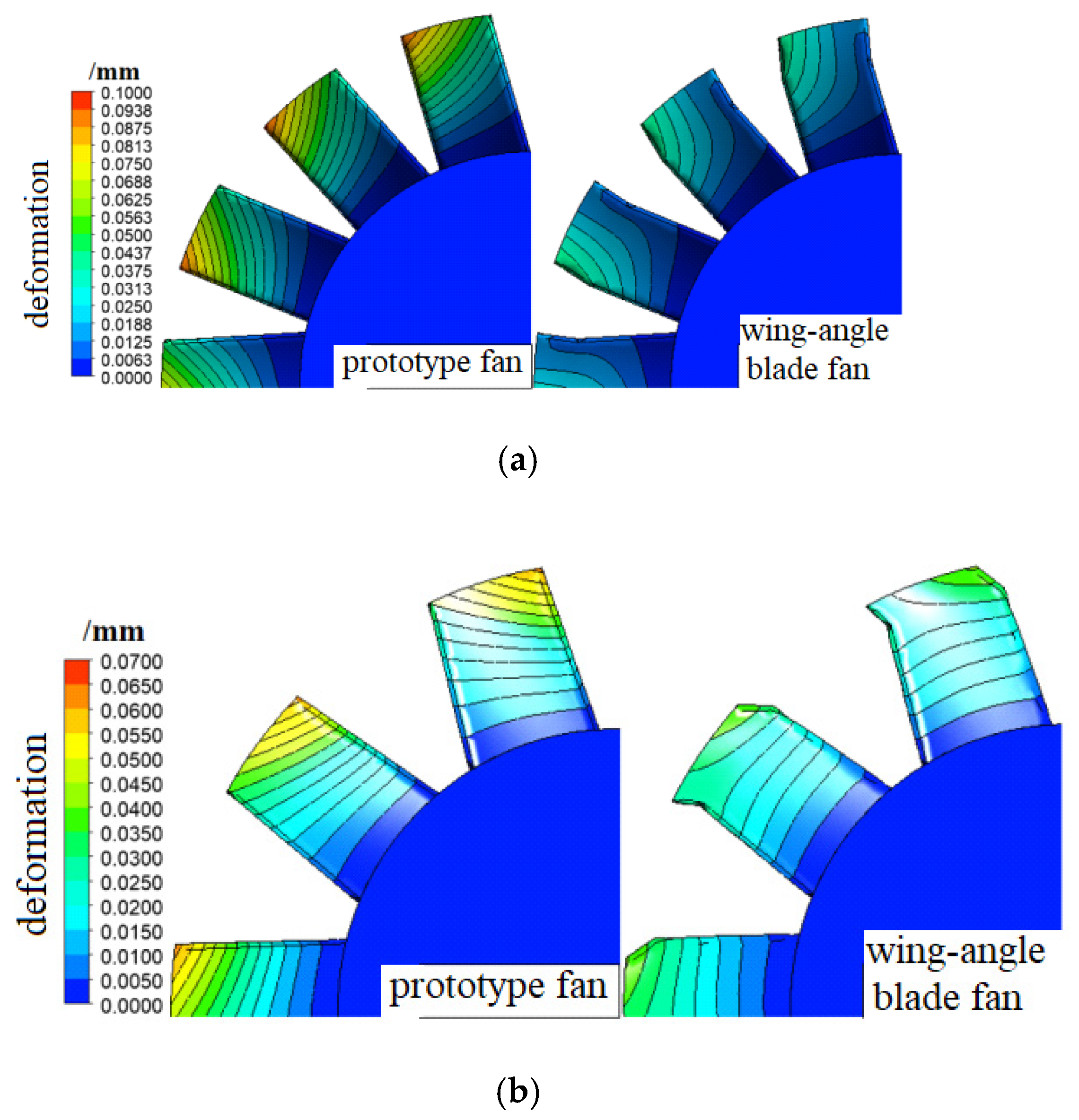
Figure 14 shows the deformation of the prototype fan and the angle blade fan at the first and second blades. Deformation of the first and second blades mainly occurs in the upper middle area of the leading edge of the blade, due to the stronger airflow impact on the leading edge than other parts of the blade, and the largest centrifugal force at this location. As summarized in Table 7, the deformation of the wing angle blade is lower than that of the prototype fan.
6. Conclusions
The following conclusions can be drawn from this study:
- (1)
- The pressure distribution on the pressure surface of the secondary blade of the optimal wing angle blade fan is stronger than that of the prototype blade. Additionally, the maximum pressures at blade heights of 25%, 50%, and 75% are increased by 2.3%, 9.3%, and 8.1%, respectively, compared with the prototype blades at the same blade height.
- (2)
- The angle blade can effectively reduce the generation of shedding vortices at the trailing edge of the blade, and reduce the strength of the shedding vortex, so that the entropy production of the optimal angle blade fan in the orthogonal experiment is reduced by 1.55% compared with the prototype fan.
- (3)
- Compared with the prototype fan, the total pressure and efficiency of the optimal wing angle blade fan are increased by 7.24% and 1.76% at the rated flow, and the total pressure and efficiency are increased by 11.32% and 3.88% on average under the full flow condition.
- (4)
- In the orthogonal experiment, the maximum sound power levels of the first and second blade trailing edge regions of the optimal wing angle blade fan were reduced by 0.17% and 1.62%, respectively, compared with the prototype fan.
Author Contributions
Conceptualization, G.G., Z.K. and Q.Y.; methodology, X.Z.; software, X.Z.; validation, G.G., Z.K. and X.Z.; formal analysis, X.Z.; investigation, G.G., X.Z.; resources, Z.K.; data curation, G.G., X.Z.; writing—original draft preparation, G.G., X.Z., X.G.; writing—review and editing, G.G., X.G.; visualization, G.G., X.Z.; supervision, Z.K., Q.Y.; project administration, Z.K., Q.Y. All authors have read and agreed to the published version of the manuscript.
Funding
This research received no external funding.
Institutional Review Board Statement
This studies do not involve humans or animals.
Informed Consent Statement
No involving humans.
Data Availability Statement
Not applicable.
Acknowledgments
The authors gratefully acknowledge the financial support of Nature fund of Chongqing Science and Technology Bureau (No. cstc2020jcyj-msxmX0793) and the Research plan projectof Chongqing Education Committee (No. KJQN202003402).
Conflicts of Interest
The authors declare no conflict of interest.
References
- Jin, Y.P.; Liu, D.S.; Wen, Z.J. Optimization design for skew and sweep parameters of mine contra-rotation two-stage blades. J. China Coal Soc. 2010, 35, 1754–1759. [Google Scholar]
- Wang, C.; Huang, L. Passive Noise Reduction for a Contrarotating Fan. J. Turbomach. 2014, 45578, V01AT10A011. [Google Scholar] [CrossRef]
- Wang, C. Trailing Edge Perforation for Interaction Tonal Noise Reduction of a Contra-Rotating Fan. J. Vib. Acoust. 2018, 140, VIB-17-1296. [Google Scholar] [CrossRef]
- Wu, Y.; Jin, Y.; Jin, Y.; Wang, Y.; Zhang, L. Effect of Hub-Ratio on Performance of Asymmetric Dual-Rotor Small Axial Fan. Open J. Fluid Dyn. 2013, 3, 81–84. [Google Scholar] [CrossRef] [Green Version]
- Mistry, C.; Pradeep, A. Effect of variation in axial spacing and rotor speed combinations on the performance of a high aspect ratio contra-rotating axial fan stage. Proc. Inst. Mech. Eng. Part A J. Power Energy 2013, 227, 138–146. [Google Scholar] [CrossRef]
- Tian, W.; Liu, F.; Cong, Q.; Liu, Y.; Ren, L. Study on aerodynamic performance of the bionic airfoil based on the swallow’s wing. J. Mech. Med. Biol. 2013, 13, 1340022. [Google Scholar] [CrossRef]
- Sun, S.M.; Xu, C.Y.; Ren, L.Q.; Zhang, Y.Z. Experimental research on noise reduction of bionic axial fan blade and mechanism analysis. J. Jilin Univ. (Eng. Technol. Ed.) 2009, 39, 382–387. [Google Scholar]
- Liang, G.Q. Experimental Research on Noise Reduction of Bionic for Axial Flow Fan. Mach. Des. Res. 2010, 26, 132–137. [Google Scholar]
- Xu, K.; Qiao, W.; Ji, L.; Chen, W. An experimental investigation on the near-field turbulence for an airfoil with trailing-edge serrations at different angles of attack. J. Acoust. Soc. Am. 2014, 135, 2376. [Google Scholar]
- Xu, K.; Qiao, W.; Ji, L.; Chen, W. An experimental investigation on the near-field turbulence for an airfoil with trailing-edge serrations and an owl specimen. J. Acoust. Soc. Am. 2013, 133, 3589. [Google Scholar] [CrossRef]
- Yakhot, V.; Smith, L.M. The renormalization group, the ε-expansion and derivation of turbulence models. J. Sci. Comput. 1992, 7, 35–61. [Google Scholar] [CrossRef]
- Guo, P.; Cao, S.G.; Zhang, Z.G.; Li, Y.; Liu, Y.B.; Li, Y. Analysis of solid-gas coupling model and simulation of coal containing gas. J. China Coal Soc. 2012, 37, 330–335. [Google Scholar]
- Xin, Z.H.; Gui, G.A.; Yu, Q.; Li, X. The Influence of Serrated Leading Edge Blade on Aerodynamic Performance of Counter-rotating Axial Fan. Chin. Hydraul. Pneum. 2020, 9, 87–92. [Google Scholar]
- Liu, T.; Kuykendoll, K.; Rhew, R.; Jones, S. Avian Wing Geometry and Kinematics. AIAA J. 2006, 44, 954–963. [Google Scholar] [CrossRef]
- Dong, J.Y.; Yang, J.H.; Yang, G.X.; Wu, F.Q.; Liu, H.S. Research on similar material proportioning test of model test based on orthogonal design. J. China Coal Soc. 2012, 37, 44–49. [Google Scholar]
- Li, C.; Zhang, C.; Zhang, R.; Ye, X. Effects of Gurney Flap on the Performance of a Variable Pitch Axial Flow Fan. J. Chin. Soc. Power Eng. 2020, 40, 404–411. [Google Scholar]
- Mariotti, A.; Buresti, G.; Salvetti, M.V. Separation delay through contoured transverse grooves on a 2D boat-tailed bluff body: Effects on drag reduction and wake flow features. Eur. J. Mech. B Fluids 2019, 74, 351–362. [Google Scholar] [CrossRef]
- Alavi Moghadam, S.M.; Loosen, S.; Meinke, M.; Schröder, W. Reduced-order analysis of the acoustic near field of a ducted axial fan. Int. J. Heat Fluid Flow 2020, 85, 108657. [Google Scholar] [CrossRef]
- Rocchio, B.; Mariotti, A.; Salvetti, M.V. Flow around a 5:1 rectangular cylinder: Effects of upstream-edge rounding. J. Wind Eng. Ind. Aerodyn. 2020, 204, 104237. [Google Scholar] [CrossRef]
- Son, J.S.; Hanratty, T.J. Numerical solution for the flow around a cylinder at Reynolds numbers of 40, 200 and 500. J. Fluid Mech. 2006, 35, 369–386. [Google Scholar] [CrossRef]
- Inoue, M.; Kuroumaru, M. Structure of tip clearance flow in an isolated axial compressor rotor. J. Turbomach. 1989, 111, 250–256. [Google Scholar] [CrossRef]
- Wang, S.; Zhang, L.; Ye, X.; Wu, Z. Performance Optimization of Centrifugal Fan Based on Entropy Generation Theory. Proc. Chin. Soc. Elect. Eng. 2011, 31, 86–91. [Google Scholar]
- Liu, H.; Ye, X.; Fan, F.; Li, C. Effects of Guide Vane Installation Angle on Performance and Static Structure of Twin-stage Variable-pitch Axial Fan. J. North China Electr. Power Univ. (Nat. Sci. Ed.) 2019, 46, 92–100. [Google Scholar]
- Chen, X.; Cao, L.; Yan, P.; Wu, P.; Wu, D. Effect of meridional shape on performance of axial-flow fan. J. Mech. Sci. Technol. 2017, 31, 5141–5151. [Google Scholar] [CrossRef]
- Kock, F.; Herwing, H. Local entropy production in turbulent shear flows: A high-Reynolds number model with wall functions. Heat Mass Transf. 2004, 47, 2205–2215. [Google Scholar] [CrossRef]
- Liu, G.; Wang, L.; Liu, X. Numerical investigation on effects of blade tip winglet on aerodynamic and aero acoustic performance of axial flow fan. J. Xi’an Jiaotong Univ. 2020, 54, 104–112. [Google Scholar]
Figure 1.
Three-dimensional model of wind turbine.
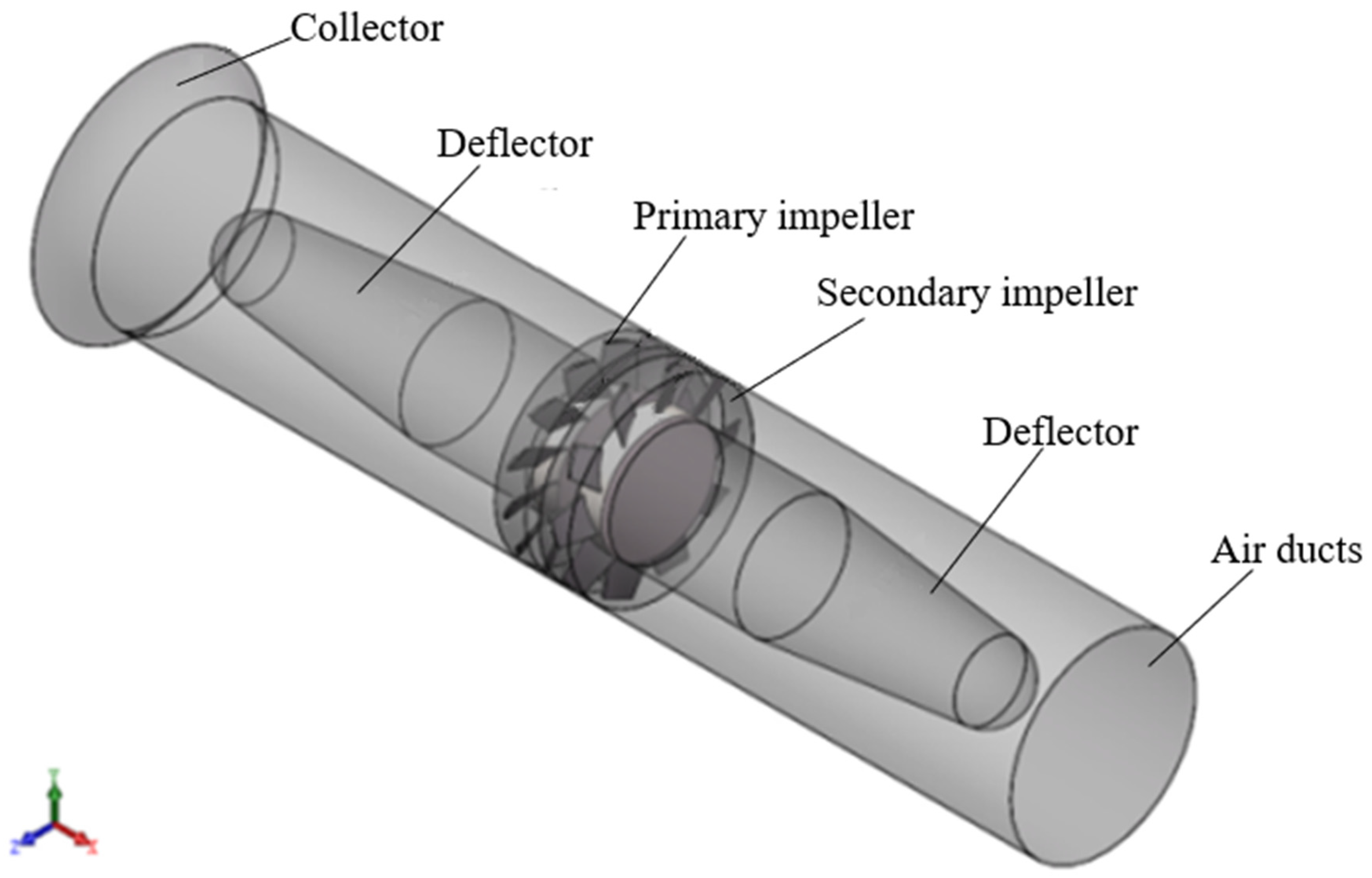
Figure 2.
Test platform for contra-rotating axial fan. (a) Counter-rotating fan and test air duct; (b) tapered restrictor.
Figure 2.
Test platform for contra-rotating axial fan. (a) Counter-rotating fan and test air duct; (b) tapered restrictor.
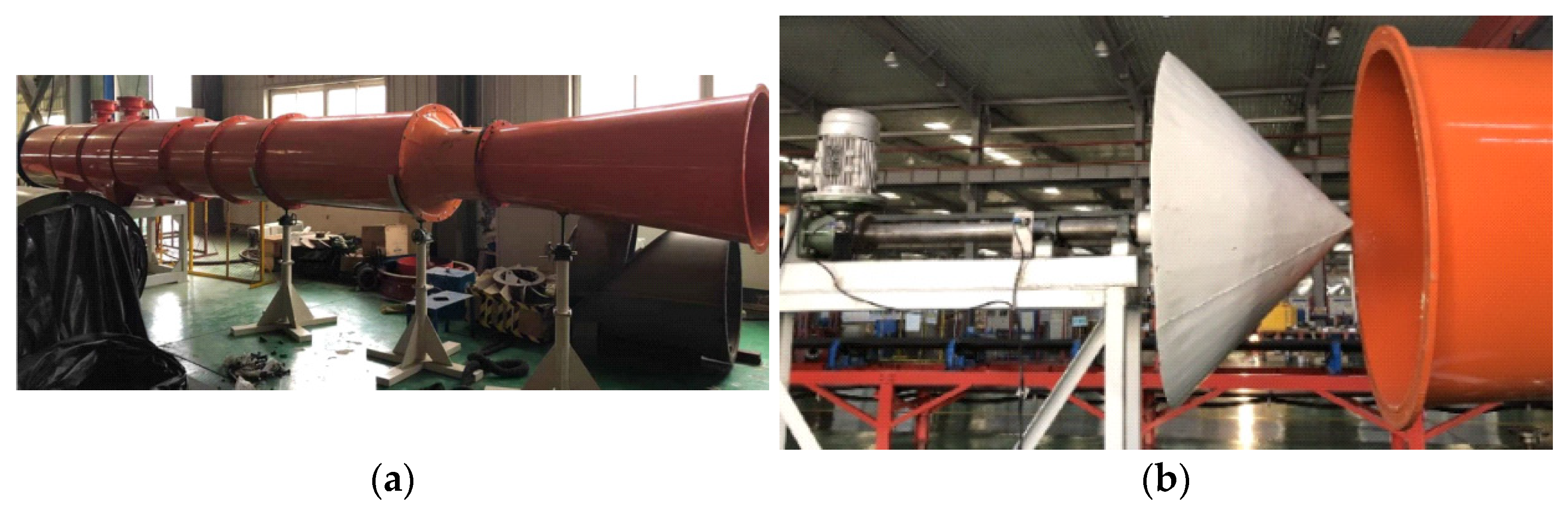
Figure 3.
Comparison of fan experiment and simulation data.
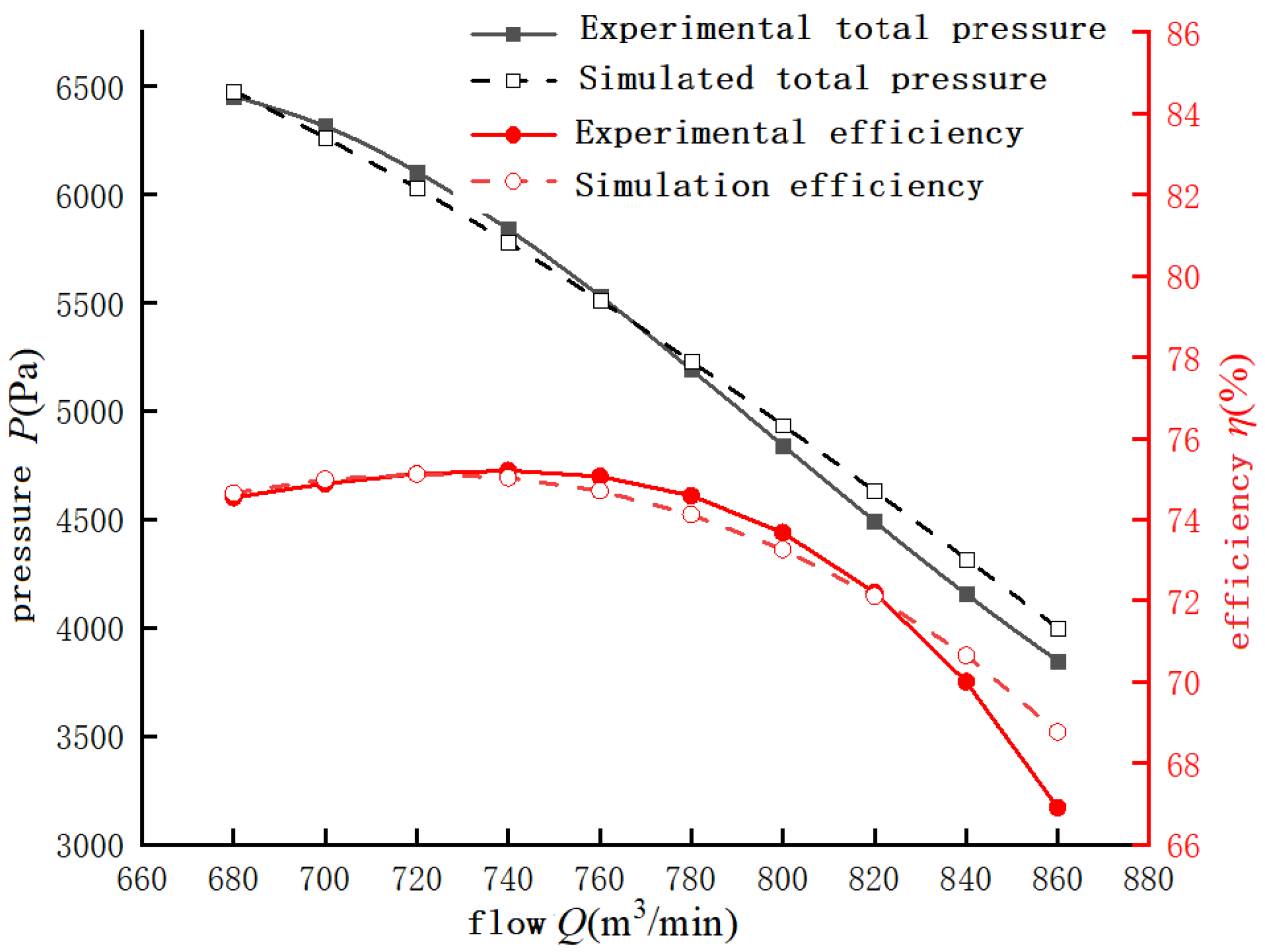
Figure 4.
Wing angle structure of bird wing.
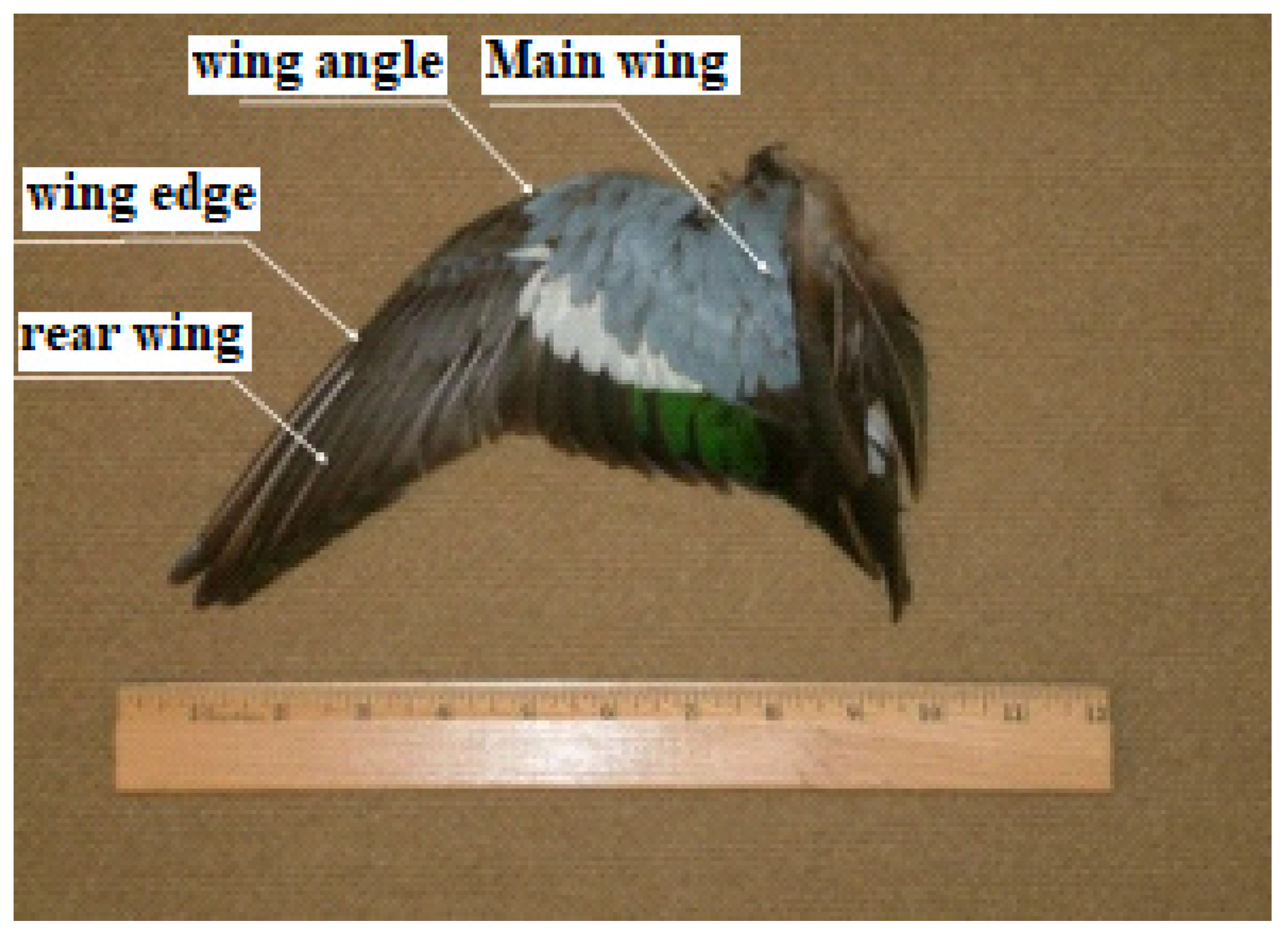
Figure 5.
Blade model.

Figure 6.
Total pressure distribution on blade surface. (a) Total pressure distribution of the first-stage blade; and (b) total pressure distribution of the second-stage blades.
Figure 6.
Total pressure distribution on blade surface. (a) Total pressure distribution of the first-stage blade; and (b) total pressure distribution of the second-stage blades.

Figure 7.
Q isosurface distribution. (a) First-stage blade of prototype fan; (b) first-stage blade of wing angle fan; (c) second-stage blade of the prototype fan; and (d) second-stage blade of wing angle fan.
Figure 7.
Q isosurface distribution. (a) First-stage blade of prototype fan; (b) first-stage blade of wing angle fan; (c) second-stage blade of the prototype fan; and (d) second-stage blade of wing angle fan.


Figure 8.
Distribution of plane A, B, and C positions.
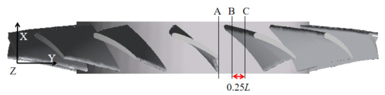
Figure 9.
Static pressure distribution on plane A, B, and C. (a) Static pressure distribution at the section of the first-stage impeller; and (b) static pressure distribution at the section of the second-stage impeller.
Figure 9.
Static pressure distribution on plane A, B, and C. (a) Static pressure distribution at the section of the first-stage impeller; and (b) static pressure distribution at the section of the second-stage impeller.
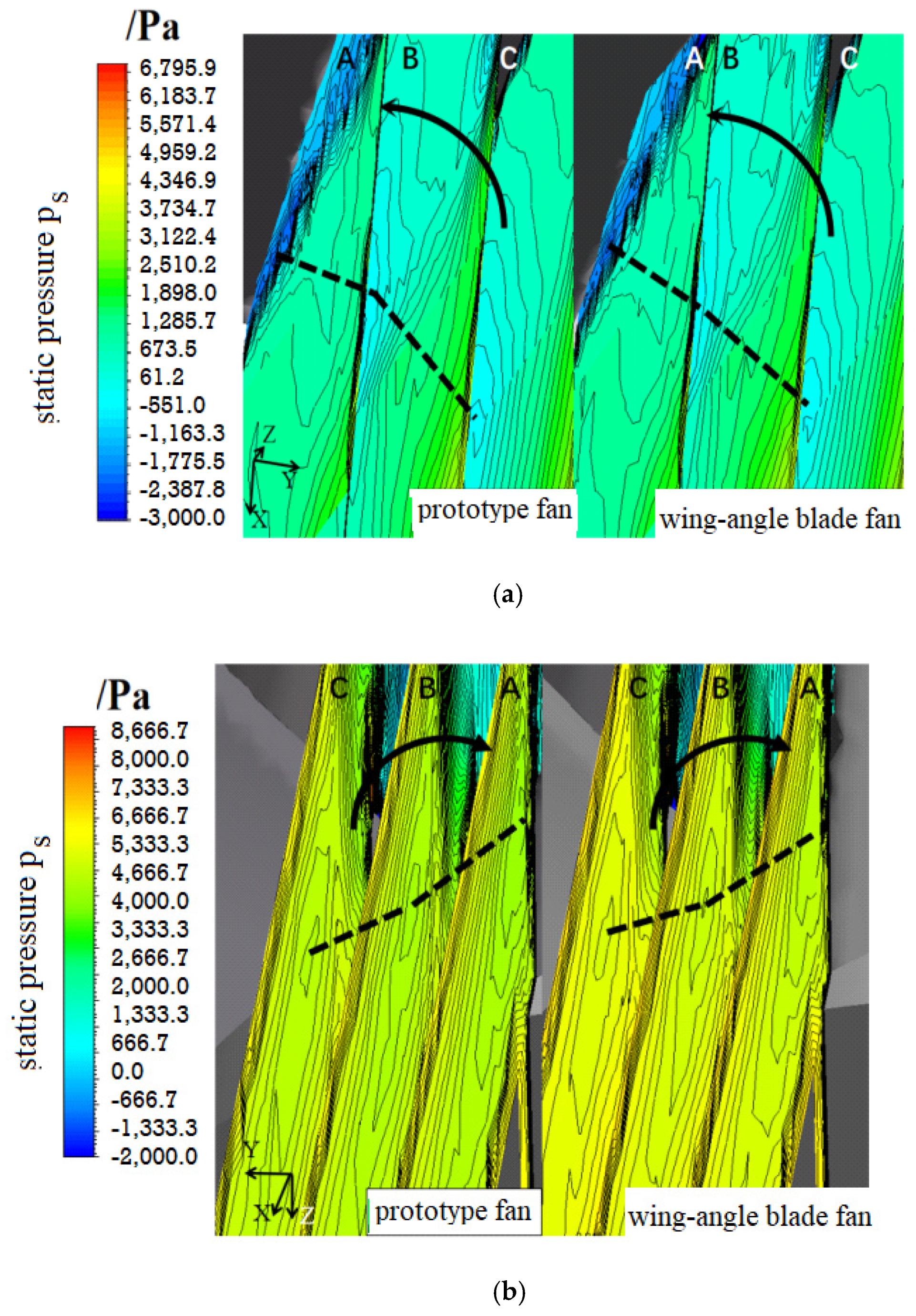
Figure 10.
S distribution of total entropy production on the blade surface. (a) S distribution of total entropy yield in the first-stage blade; and (b) S distribution of total entropy yield in the second-stage blade.
Figure 10.
S distribution of total entropy production on the blade surface. (a) S distribution of total entropy yield in the first-stage blade; and (b) S distribution of total entropy yield in the second-stage blade.

Figure 11.
Full flow analysis.

Figure 12.
Sound power distribution in the trailing edge area of the first and second stage blades. (a) Sound power distribution in the trailing edge area of the first-stage blade; and (b) sound power distribution in the trailing edge area of the second-stage blade.
Figure 12.
Sound power distribution in the trailing edge area of the first and second stage blades. (a) Sound power distribution in the trailing edge area of the first-stage blade; and (b) sound power distribution in the trailing edge area of the second-stage blade.
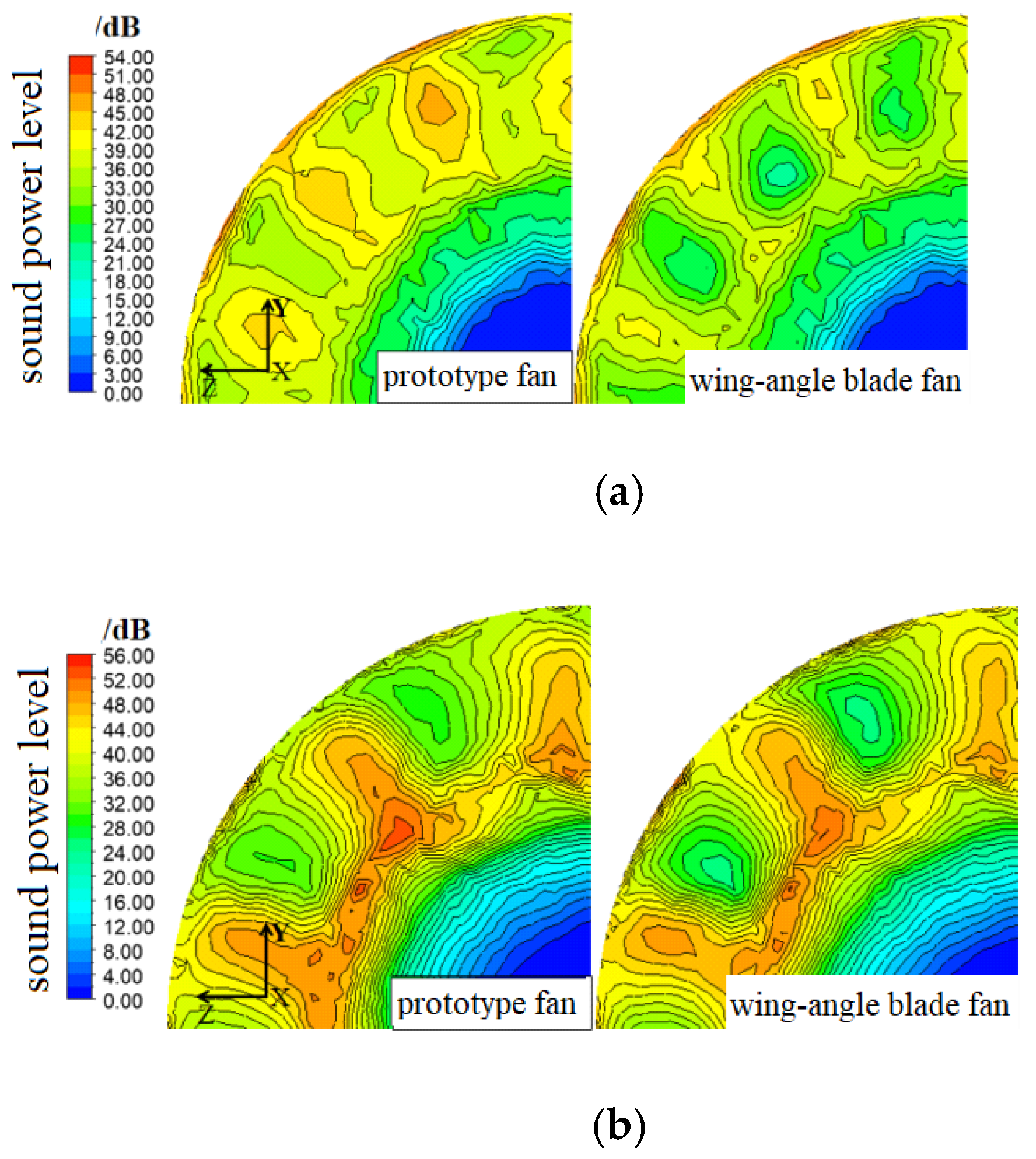
Figure 13.
Comparison of equivalent distribution of wing angle blades and prototype wind turbines. (a) Equivalent stress on pressure surface of the first-stage blade; (b) equivalent stress on the suction surface of the first-stage blade; (c) equivalent stress on pressure surface of the second-stage blade; and (d) equivalent stress on the suction surface of the second-stage blade.
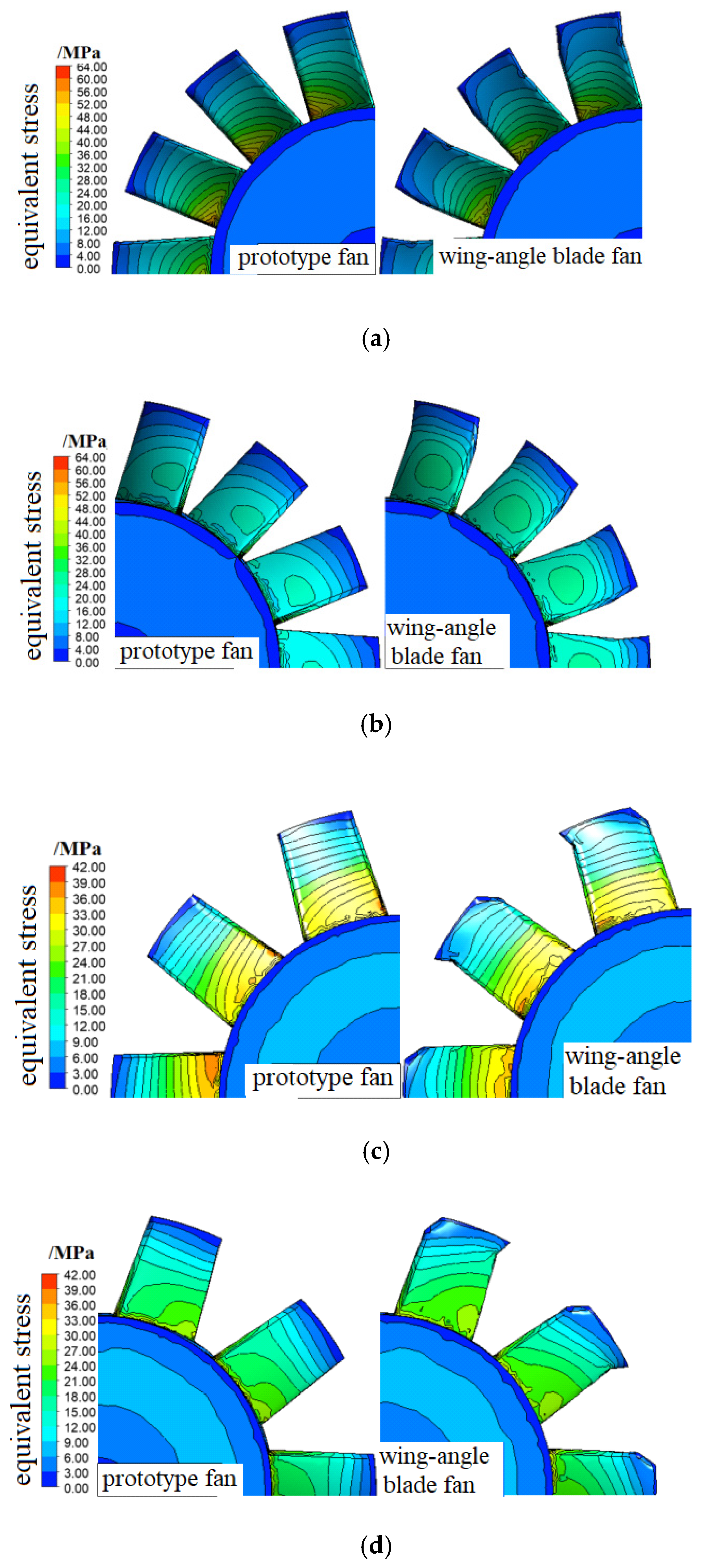
Figure 14.
Deformation distribution of wing angle blades and prototype blades. (a) First-stage blade deformation distribution; and (b) second-stage blade deformation distribution.
Figure 14.
Deformation distribution of wing angle blades and prototype blades. (a) First-stage blade deformation distribution; and (b) second-stage blade deformation distribution.

Table 1.
Design parameters of FBD No.8.0 mine cyclone machine.
| Design Parameters | Value |
|---|---|
| Number of blades of first-stage impeller | 14 |
| Number of blades of second-stage impeller | 10 |
| One, two leaf height (H/mm) | 150 |
| Chord length of first and second stage blade tip (L/mm) | 111 |
| One, two wheel hub ratio | 0.6 |
| One, two stage tip clearance(mm) | 2 |
| One, two rated speed/(rad/min) | ±2900 |
| Mounting Angle of first-stage blade (°) | 46 |
| Mounting Angle of two-stage blade (°) | 30 |
Table 2.
Grid independence test.
| The Number of Cells (Million) | The Efficiency (%) | The Number of Cells (Million) | The Efficiency (%) |
|---|---|---|---|
| 1.34 | 72.23 | 1.70 | 71.98 |
| 1.79 | 73.25 | 2.02 | 74.62 |
| 3.22 | 74.50 | 3.64 | 74.56 |
Table 3.
Orthogonal experiment factors level table.
| Test Serial Number | Position of First-Stage Blade Angle A/mm | Tip Offset Distance of First-Stage Blade B/mm | Position of Second-Stage Blade Angle C/mm | Offset Distance of Blade Tip of Second-Stage Impeller D/mm |
|---|---|---|---|---|
| 1 | 100 | 10 | 100 | 10 |
| 2 | 110 | 15 | 110 | 15 |
| 3 | 120 | 20 | 120 | 20 |
Table 4.
Design flow point efficiency data processing and range analysis.
| Test Serial Number | Position of First-Stage Blade Angle A/mm | Tip Offset Distance of First-Stage Blade B/mm | Position of Second-Stage Blade Angle C/mm | Tip Offset Distance of Second-Stage Blades B/mm | Efficiency η/% |
|---|---|---|---|---|---|
| 1 | 100 | 10 | 100 | 10 | 76.69 |
| 2 | 100 | 15 | 110 | 15 | 76.36 |
| 3 | 100 | 20 | 120 | 20 | 76.94 |
| 4 | 110 | 10 | 110 | 20 | 76.53 |
| 5 | 110 | 15 | 120 | 10 | 76.45 |
| 6 | 110 | 20 | 100 | 15 | 76.38 |
| 7 | 120 | 10 | 120 | 15 | 76.51 |
| 8 | 120 | 15 | 100 | 20 | 76.32 |
| 9 | 120 | 20 | 110 | 10 | 76.31 |
| k1 | 77.66 | 76.58 | 76.46 | 76.48 | |
| k2 | 76.45 | 76.38 | 76.40 | 76.42 | |
| k3 | 76.38 | 76.54 | 76.63 | 76.60 | |
| Range | 0.28 | 0.20 | 0.23 | 0.18 |
Table 5.
Entropy production in each area of the angle blade fan and the prototype fan.
| Type | Entropy Production | Wind Tube | Primary Impeller | Secondary Impeller | Total |
|---|---|---|---|---|---|
| Prototype fan | 0.1186 | 2.2784 | 4.1418 | 6.5388 | |
| 1.1334 | 29.7861 | 41.4495 | 72.3690 | ||
| 1.2520 | 32.0645 | 45.5913 | 78.9078 | ||
| Wing angle blade fan | 0.1150 | 2.2760 | 4.2264 | 6.6174 | |
| 1.0972 | 29.6556 | 40.3174 | 71.0702 | ||
| 1.2122 | 31.9316 | 44.5438 | 77.6876 |
Table 6.
Equivalent stress of blade.
| Blade Stage | Prototype Fan | Wing Angle Blade Fan | ||
|---|---|---|---|---|
| Minimum Equivalent Stress/MPa | Maximum Equivalent Stress/MPa | Minimum Equivalent Stress/MPa | Maximum Equivalent Stress/MPa | |
| First-stage blade | 0.0008 | 61.8577 | 0.0011 | 53.2365 |
| Second-stage blade | 0.0048 | 40.0064 | 0.0046 | 40.4835 |
Table 7.
Maximum deformation of the blade.
| Blade Stage | Maximum Deformation/mm | |
|---|---|---|
| Prototype Fan | Wing Angle Blade Fan | |
| First-stage blade | 0.0969 | 0.0463 |
| Second-stage blade | 0.0624 | 0.0411 |
Publisher’s Note: MDPI stays neutral with regard to jurisdictional claims in published maps and institutional affiliations. |
© 2022 by the authors. Licensee MDPI, Basel, Switzerland. This article is an open access article distributed under the terms and conditions of the Creative Commons Attribution (CC BY) license (https://creativecommons.org/licenses/by/4.0/).
Share and Cite
MDPI and ACS Style
Gao, G.; You, Q.; Kou, Z.; Zhang, X.; Gao, X. Simulation of the Influence of Wing Angle Blades on the Performance of Counter-Rotating Axial Fan. Appl. Sci. 2022, 12, 1968. https://doi.org/10.3390/app12041968
AMA Style
Gao G, You Q, Kou Z, Zhang X, Gao X. Simulation of the Influence of Wing Angle Blades on the Performance of Counter-Rotating Axial Fan. Applied Sciences. 2022; 12(4):1968. https://doi.org/10.3390/app12041968
Chicago/Turabian StyleGao, Guijun, Qingshan You, Ziming Kou, Xin Zhang, and Xinqi Gao. 2022. "Simulation of the Influence of Wing Angle Blades on the Performance of Counter-Rotating Axial Fan" Applied Sciences 12, no. 4: 1968. https://doi.org/10.3390/app12041968
Note that from the first issue of 2016, this journal uses article numbers instead of page numbers. See further details here.