
Isolating the Role of the Transport System in Individual Accessibility Differences: A Space-Time Transport Performance Measure


1
Faculty of Architecture and Spatial Planning, Vienna University of Technology, Karlsgasse 11, A-1040 Vienna, Austria
2
Eurac Research, Institute for Regional Development, Viale Druso 1, I-39100 Bolzano, Italy
*
Authors to whom correspondence should be addressed.
Appl. Sci. 2022, 12(7), 3309; https://doi.org/10.3390/app12073309
Submission received: 18 February 2022
/
Revised: 16 March 2022
/
Accepted: 21 March 2022
/
Published: 24 March 2022
(This article belongs to the Special Issue Future Transportation)
Abstract
:Accessibility differences across individuals are a core topic in the transport equity debate. Space-Time Accessibility measures (STAs) have often been used to show such differences, given their sensitiveness to individual spatial and temporal constraints. However, given their complexity, STAs cannot properly isolate the specific role of the transport system in individual accessibility differences, since it is mixed with several other spatial, individual and temporal factors. To isolate the role of the transport system, this study introduces a Space-Time Transport Performance measure (STTP) that (a) grounds on the individual daily schedule of fixed activities, (b) calculates the generalised transport costs each individual has to bear to perform such schedule, and (c) weights it against the Euclidean distance between the activities of such a schedule. STTP is tested together with STA for a small sample of individuals living and performing their daily activities within the 22nd district of Vienna. This test provides two main findings: first, individual differences registered by STTP tend to be smaller than those highlighted by STA, according to the former’s more narrowed and transport-specific approach. Second, individuals with the highest STA do not necessarily register the highest STTP (and vice versa). Indeed, some may experience limited transport performances when running their mandatory daily schedule, while registering a high degree of access to discretionary activities according to their constraints and opportunities at disposal (and vice versa). Considering these results, STTP may be seen as a complementary indicator to be used together with STA to analyse both general and transport-specific individual accessibility differences. Its role is particularly important for transport policy makers, who should understand which accessibility differences are directly linked to the performances of the transport system and could be remediated through transport policies.
1. Introduction
As highlighted by van Wee and Mouter [1], “in the transport policy literature, there is consensus that ‘sound’ policies have to meet three criteria: they should be effective, efficient and fair” [2]. Effectiveness and efficiency have received significant attention in the last decades [1], while the same does not apply to fairness except for contributions addressing social exclusion (e.g., ref. [3]). In recent years, the attention on transport fairness has increased thanks to the growing importance of inequality reduction at the international level, e.g., among the Sustainable Development Goals of the United Nations [4]. The lack of studies in this field is linked to the normative nature of fairness, making it difficult to measure and apply it to a cost–benefit analysis (one of the most diffused policy assessment tools [1,5]). Due to this normative issue, most studies in transport fairness focus on distributional analyses, i.e., how transport effects (such as air pollution variations or safety variations) are distributed over people [1,6]. One of the most addressed effects is the variation of individual accessibility differences [5]. Indeed, accessibility is one of the critical pillars for a sustainable mobility paradigm [7]. Its improvement is one of the core concerns for transportation ministries throughout the world [8].
However, most accessibility measures developed in the literature are not suitable to point out such individual differences since they focus on the physical separation among places and overlook the accessibility differences that could exist among people living in the same area (e.g., because of their different modal restrictions or daily schedules [9]). To fill this gap, so-called person-based accessibility measures have been developed [10,11]. Among them, the Space-Time Accessibility measure (STA) is one of the most diffused given its sensitiveness to individual space-time constraints [12,13,14]. Although STA is very suitable for investigating individual accessibility differences in general, its high complexity does not allow a clear understanding of the specific role the transport system plays in such differences, differences which are fed by a multitude of spatial, transport, individual and temporal factors. This is a relevant limit of STA especially from the perspective of transport policy makers, who should introduce transport policies aimed at reducing such differences. Indeed, accessibility differences are often unavoidable and the transport system cannot remediate them [1]. For instance, inevitably, people living close to a large facility (e.g., a hospital) have better access to it than people living far away. However, this is unavoidable due to land-use constraints (hospitals cannot be built in any municipality), and transport policies cannot eliminate distance. Given this issue, it is necessary to complement STA with transport performance measures (With the term “transport performance” we mean a set of transport indicators that describe the efficiency of the transport system, such as commercial speed, network capacity, service period, average waiting or transfer time, or monetary cost of travel) able to isolate the specific role of the transport system in individual accessibility differences, which could be avoided or remediated through transport policy interventions. For this purpose, this paper introduces a so-called Space-Time Transport Performance measure (hereinafter STTP).
The rest of the article is organised as follows. Section 2 reviews main place- and person-based accessibility measures used in literature and points out the elements that prevent STA from isolating the role of the transport system in individual accessibility differences. On this basis, Section 3 introduces STTP by describing its key features and its computation process. STTP is then tested in Section 4 together with STA to determine the complementary results that are achievable with the proposed measure. Moreover, it discusses the limits of STTP. Section 5 concludes the contribution by highlighting potential contexts of application.
2. Place- and Person-Based Accessibility Measures
In general terms, place-based measures calculate accessibility for a location by assuming that all people in that location register the same accessibility. Conversely, person-based calculations analyse accessibility for individuals living in the same area to understand how accessibility varies across them [15]. Section 2.1 and Section 2.2 summarise the main place- and person-based measures developed and used in literature, while Table 1 displays their definition, mathematical formulation and main conceptual and operational pros and cons. Afterwards, Section 2.3 discusses the factors that prevent STA from isolating the role of the transport system in individual accessibility differences.
2.1. Place-Based Measures
Place-based measures calculate how easy it is for people departing from a place to reach opportunities located in another [9,16]. Following this definition, three main types of place-based measures have been developed: cumulative-opportunity, gravity-based and adapted gravity-based measures ([9,17]; Table 1). All of these are a function of two core elements: (a) an attraction factor given by the amount, spatial distribution and quality of opportunities to access; and (b) an impedance factor given by the effort needed to reach these opportunities [18]. These are combined in different ways. The cumulative-opportunity measure (e.g., refs. [19,20,21]) counts the number of opportunities reachable from an origin location within a predetermined threshold usually defined in terms of travel time or cost. It is a very straightforward approach, but it shows some limits since counted opportunities have the same importance regardless of the effort needed to reach them. The gravity-based measure (e.g., refs. [22,23,24]) addresses these limits since it calculates the accessibility of an origin as a function of the number and importance of opportunities at the destination, weighed against the travel effort needed to reach them. However, it neglects the competition between the demand for and supply of opportunities. The adapted gravity-based measure (e.g., refs. [25,26,27]) incorporates them through a double constrained spatial interaction model with two mutually-dependent balancing factors [17].
These three measures have two main limitations that person-based measures aim to overcome [13,28]. First, they assume that all individuals who depart from the same origin location experience the same level of accessibility regardless of their different spatial, temporal and modal constraints. Second, they calculate accessibility for a single reference location (typically home place) overlooking the fact that people generally perform a sequence of daily activities that are differently located in space and time, and this sequence affects their accessibility.
2.2. Person-Based Measures
Three main types of person-based measures address the gaps of the place-based measures: the utility-based, individual integral and space-time measures ([11,17]; Table 1). The utility-based measure (e.g., refs. [9,29,30]) grounds on economic theories and calculates accessibility as the maximal economic utility individuals can get from the access to spatially distributed opportunities based on their perception of the utility of the options at their disposal. The individual integral measure (e.g., refs. [31,32,33]) is a gravity-based measure adjusted to be person-specific. The adjustment is performed either by disaggregating data and analysis by, e.g., trip purposes, transport modes, age or income groups; or by using a non-zonal method as the point-based approach, which allows a focus on specific point locations and measurement of point-to-point travel costs at the individual level. Although person-based, this last measure focuses on a single reference location, and it overlooks the spatio-temporal constraints affecting people on a daily basis [34]. The space-time measure addresses these limitations in the most comprehensive manner (e.g., refs. [14,35,36]).
For this reason, this is considered an effective approach to measure accessibility at the individual level and to discuss individual accessibility differences [10]. It derives from the time geography framework elaborated by Hägerstrand [37] and focuses on the set of discretionary opportunities (i.e., non-mandatory daily activities) that individuals could reach on a daily basis given the spatio-temporal constraints posed by their fixed daily activity chain (i.e., mandatory daily activities) [38]. This set is called a Feasibility Opportunity Set (FOS), and is obtained in three steps. First, the daily sequence of fixed activities constrained in space and time for a person is schematised. This sequence generates a so-called Space-Time Path (STPA). Based on the STPA, the Potential Path Areas (PPAs) are calculated for each couple of the following fixed activities in the STPA. Each PPA includes all the locations that an individual could visit between two subsequent fixed activities, given the mandatory departure time from the former, the mandatory arrival time at the latter, the time needed to travel between them, and the time required to visit such locations. By extending the calculation of the PPA to all couples of sequential fixed activities, the Daily Potential Path Area is obtained (DPPA). All the opportunities that belong to the DPPA constitute the FOS and define the space-time accessibility measure (STA).

Table 1.
Main place- and person-based accessibility measures and their key features.
| Accessibility Measure | General Definition | Mathematical Formulation * | Conceptual/Operational Pros | Conceptual/Operational Cons | Sample References | |
|---|---|---|---|---|---|---|
| Place-based measures | Cumulative opportunity | Set of opportunities reachable from a location within a pre-defined travel time or cost | Easily understandable and applicable | Opportunities have the same importance regardless of their features | [19,20,21] | |
| Gravity-based | Set of opportunities reachable at destination weighed by the travel effort needed to reach them | It considers the role of the travel effort in decreasing accessibility | It neglects temporal constraints and competition effects | [22,23,24]. | ||
| Adapted gravity-based | Gravity-based measure including competition effects between demand for and supply of opportunities | It includes competition effects between demand for and supply of opportunities | Particularly difficult to operationalize and adopt in concrete analyses | [25,26,27]. | ||
| Person-based measures | Utility-based | Maximal economic utility individuals can get from the access to spatially distributed opportunities | Utility is measured at individual level and results can feed economic evaluations | Temporal constraints are neglected while results are not easily understandable | [9,29,30] | |
| Individual integral | Gravity-based measure adapted to analyse individual accessibility through disaggregation or point-based approach | It allows focusing on e.g., specific trip purposes, transport modes, or age groups | It measures accessibility for a single location and neglects spatio-temporal constraints | [31,32,33] | ||
| Space-time | Set of opportunities reachable by an individual according to his/her daily activity programme and constraints | Sensitive to individual transport specificities and spatio-temporal constraints | It needs peculiar input data and skip transport factors beyond travel time | [14,35,36] | ||
* Where: Cumulative opportunity: i is an origin location; j is a destination location; Oj are the opportunities available at destination; TCij is the cost of travelling from i to j; f(TCij) is the travel cost function, which may assume different forms such as linear, Gaussian, logistic or negative exponential; T is the travel cost threshold set in the analysis. Gravity-based: i, j, Oj, TCij and f(TCij) are defined above. Adapted gravity-based: i, j, Oj, TCij and f(TCij) are defined above; ai is the balancing factor for demand in location i; bj is the balancing factor for supply in location j; Di is the demand for opportunities in i. Utility-based: u is a user for whom accessibility is calculated; λ is the travel cost coefficient; z is one of the choices that u can make; Cu is the set of choices z that u can make; Vzu is the systematic utility of the choice z for u. Individual integral: u, i, j, Oj and f(TCij) are defined above; TCiju,k is the travel cost for u from i to j by transport mode k. Space-time: u is defined above; w1−n are the locations of discretionary opportunities; Ow are the discretionary opportunities Ow available in w1−n; DPPA is the Daily Potential Path Area; t is the time needed to participate in a discretionary opportunity Ow; ta is the ending time of a fixed activity a; ta+1 is the starting time of the following fixed activity a+1; da,w is the physical distance between a and w; dw,a+1 is the physical distance between w and a+1; v is the average speed on the transport network.
2.3. Limits of STA in Describing the Role of the Transport System
Thanks to its individual sensitiveness and capacity to comprise all the four accessibility components (land-use, transport, individual and temporal; [17]), STA is often adopted in the analysis of accessibility differences (e.g., refs. [10,12,39]). Nevertheless, STA presents some limits when it comes to isolating the role of the transport system in individual accessibility differences. In particular:
- Limited relevance of the transport system performances in the FOS: STA is represented by the FOS, which mostly depends on the amount and spatial distribution of the discretionary opportunities and the spatio-temporal constraints of the STPA [11]. Therefore, STA focuses highly on spatial and temporal accessibility components and less on transport performances [17]. This is a gap when the aim is to isolate the specific role of a transport system in individual accessibility differences. For instance, let us assume two people who both have one fixed activity during their day, departing and headed to the same locations simultaneously, and using the same transport system with the same performances. The former works full-time while the latter part-time. According to the STA concept, the different time constraints of the two individuals would lead to an accessibility difference since the part-time worker has more occasions to engage in discretionary activities than the full-time worker. However, the performance of the transport system does not play a role in such accessibility differences.
- Unsuitability of the FOS to represent accessibility differences: As stressed by Pritchard et al. [40,41], the choice of the accessibility measure may significantly influence the outcomes of the analysis. Therefore, it is crucial to deploy a measure that is as suitable as possible to discuss accessibility distribution. Specifically, the estimate should represent an optimisation factor for the observed individuals, i.e., a good they generally aim to increase [42]. This is the case, e.g., with income, which is one of the critical indicators for distributional analyses in socio-economic sciences [43]. STA cannot be easily labelled as an optimisation factor since it is not straightforward to state that individuals aim to maximise the number of discretionary opportunities they could reach on a daily basis. For instance, a person could have a small FOS because (s)he has a tight schedule of fixed activities and no room to engage in discretionary ones. Nevertheless, (s)he could be not much interested in further activities. At the same time, the transport system could be efficient in allowing them to reach all the fixed activities with a reasonable effort [5].
Based on these limits, we introduce the so-called Space-Time Transport Performance measure (STTP) in order to complement STA by isolating the role of the transport system in individual accessibility differences.
3. Space-Time Transport Performance Measure (STTP)
3.1. Key Features of STTP
STTP aims to measure the performances of the transport system based on the spatio-temporal and individual constraints characterising the daily life of each individual. To meet this purpose, STTP grounds on three key features, described below in detail.
- Focus on the Individual Daily Travel Cost (IDTC) incurred for the daily fixed activities: STTP is not focused on the sum of the discretionary opportunities potentially reachable given the schedule of fixed activities (i.e., the FOS). Instead, it focuses on the individual travel cost incurred to perform the daily schedule of fixed activities (from now on named Individual Daily Travel Cost; IDTC). IDTC is calculated as the generalised cost of transport incorporating both monetary and non-monetary cost (see Section 3.2 for further details). This shift of perspective allows STTP to focus on a factor that is transport-specific rather than land-use-specific and thus isolate the performance of the transport system. Moreover, it allows STTP to focus on an indicator that is suitable to represent transport-related accessibility differences. Indeed, individuals tend to minimise the transport cost needed to reach their fixed daily destinations [42,44]. However, by focusing on IDTC, STTP also excludes the discretionary part of accessibility typically included in STA and representing the potential for activities offered by surrounding amenities. This choice requires STTP to be complemented with STA to capture the potential component of accessibility.
- Weighting of IDTC against the Individual Daily Distance (IDD):IDTC is usually influenced by the distance daily travelled: the higher the distance, the higher IDTC. This may be misleading for evaluating individual transport-performance differences, since even in the case of identical transport performances, people who travel longer distances would be more disadvantaged than those travelling short ones. To isolate the role of the transport system performance in individual accessibility differences, this variable needs to be controlled to exclude its influence from the analysis. For this purpose, STTP weights IDTC against the Individual Daily Distance (IDD). This is the sum of the Euclidean distances between each couple of subsequent activities belonging to an individual’s daily schedule (see Section 3.2 for further details). This choice makes STTP a measure of transport performance rather than a measure of the daily transport effort of individuals (which would be influenced also by the distance daily covered).
- Estimation of IDTC based on temporal and individual constraints: To incorporate the temporal constraints, STTP calculates IDTC by considering the actual location and timing of the fixed activities daily performed by an individual. Also, the individual constraints are incorporated in the IDTC computation in two ways. First, the actual modal choices of individuals for each daily travel are considered according to individual constraints such as the ability to drive or car ownership. Second, the non-monetary cost part of IDTC (i.e., travel-time costs) are estimated at the individual level based on income (as described in detail in Section 3.2).
These three features shape STTP as a transport performance indicator that stems from spatio-temporal and individual constraints. On the one hand, this allows STTP to isolate the role of the transport system in individual accessibility. On the other hand, it suggests how STA and STTP should be deployed together to get both a comprehensive picture of space-time accessibility and more narrowed information on the transport component. Figure 1 summarises the relation between STA and STTP, while Section 3.2 describes how STTP is calculated.
3.2. Calculation of STTP
STTP (Formula (1)) is calculated by following three steps: (A) the setup of the STPA; (B) the calculation of the IDTC figures; (C) the calculation of the IDD figures.
(A) The setup of the STPA is made in the same way as for STA. The daily sequence of fixed activities (a1−n) constrained in space and time for the observed individual is schematised. This includes the location where each a takes place (address); its category (home-stay, work, education or other); the duration of each a given by its mandatory starting and ending time; the transport mode(s) usually used to travel between each couple of subsequent activities (a); and the degree of fixity for each an according to the flexibility of its location and timing. This is made through a 1–5 Likert scale, where 1 indicates maximum flexibility of the location and/or timing of a, while 5 shows a minimum one. The data needed to reconstruct the STPA are collected from observed individuals using travel diaries. Interviewed individuals are asked to fill them out by considering a typical weekday of their daily life. Table 2 shows an exemplificative (and fictional) STPA.
(B) Once the STPA is set, IDTC is calculated (Formula (2)). IDTC is the sum of the Individual Transport Costs incurred by an individual for each daily travel performed by the transport mode k between each couple of subsequent fixed activities a,a+1 (ITCka,a+1). Each ITCka,a+1 value is calculated through a generalised cost function, including a series of monetary and non-monetary (but monetizable) costs [42]. This consists of the monetary cost of travel (Cm), the cost of the in-vehicle travel time (Civtt), and the cost of out-of-vehicle travel time (Covtt). Cm encompasses the costs for the usage of infrastructures (e.g., tolls and parking fares), the operating costs of vehicles (e.g., fuel, usage-related depreciation and insurance), and the costs for access to services (e.g., public transport; from now on PT). Civtt includes the time spent within private, shared or pooled vehicles. Covtt covers the cost of the time to access the first transport system (first mile), the waiting time for transport services, the transfer time among transport services, and the time to reach the final destination (last mile [42]). Civtt and Covtt are monetised based on unitary Values of Travel Time (VTT). As demonstrated in the literature, VTT may vary by income, country, travel purpose, mode of transport and distance. It depends on the approach with which it is estimated (e.g., stated vs. revealed preference surveys [44]). The wage rate method is used for STTP: different wage rate shares are assumed depending on the country of investigation, travel purpose, and transport mode. Moreover, the actual wage rates of observed individuals are used to make the estimation individual.
(C) Once IDTC is calculated, this has to be weighed against IDD (Formula (3)). This is the sum of the distances measured between each couple of subsequent fixed activities a,a+1 (Da,a+1). Each Da,a+1 value is measured as Euclidean and not travelled distance along with the transport network. Indeed, the travelled distance may be influenced by the design of the transport system and not only by the land-use system. For instance, this is the case with fast transport systems such as motorways and high-speed railways, which tend to generate much more detours than slower systems (a phenomenon called “spatial inversion” by Bunge [45]). This detour is an aspect that transport planners can potentially address e.g., by modifying the shape of the PT lines and distribution of stops. Therefore, it is a factor to be included in the accessibility computation. Conversely, the Euclidean distance solely depends on the land-use system (i.e., the amount and location of opportunities in space) therefore it is used to weight IDTC and point out the role of the transport system in accessibility differences. Figure 2 summarises the calculation process for STA (in red) and STTP (in blue) based on STPA (in black), which is the common element between them.
where: a1−n are the fixed activities performed by an individual on a daily basis, k is the mode(s) of transport used by an individual between each couple of subsequent as, IDTC is the Individual Daily Travel Cost incurred by an individual on a daily basis, IDD is the Individual Daily Distance between the as performed by an individual on a daily basis, ITCka,a+1 is the individual transport cost by mode k between each couple of subsequent as, Cmka,a+1 is the monetary cost of transport by mode k between each couple of subsequent as, Civttka,a+1 is the cost of in-vehicle travel time by mode k between each couple of subsequent as, Covttka,a+1 is the cost of out-of-vehicle travel time by mode k between each couple of subsequent as, and Da,a+1 is the Euclidean distance between each couple of subsequent as.
4. Joint Test of STA and STTP in the City of Vienna
The test aims to show how STTP may lead to complementary results for STA, providing insights on the role of the transport system in individual accessibility differences. Similar to other studies focused on the methodological integration of the space-time approach (e.g., refs. [36,46]), we run the test for a small sample of five individuals, for whom STA and STTP are calculated. We perform such a small test for two reasons: first, because the purpose is to provide a methodological test and not to get statistically relevant results about a specific phenomenon (e.g., gender or income-related accessibility differences). Second, focusing on a few individuals allows a more detailed reflection on results, e.g., pointing out the main differences for each individual (Section 4.3). This would not be feasible with a test involving many individuals, which would be more suitable for statistical comparison. Nevertheless, focusing on such a small test also has some limits, which are discussed in Section 4.4.
4.1. Study Area and STPAs
The test is run in the City of Vienna, Austria. The analysed individuals (A–E) live and perform their fixed activities within the 22nd district (Donaustadt). This is the second northernmost district of Vienna, with the greatest surface (ca 102 km2), the second-highest population (ca 198,800 inhabitants), and the second-lowest population density out of the 23 city districts (1943 inhabitants/km2). The district is served by 26 bus lines, two light rail lines and two subway lines. Moreover, it is served by a road network that is denser in the core part of the district characterised by a higher urban density and much lower at the fringes, where green areas are predominant. Given the heterogeneous availability of transport means, the area represents a suitable case study to explore the individual accessibility differences related to the transport system. Figure 3 displays the road and PT network of the study area, the location of the available opportunities, the location of the home places, and the fixed activities of the individuals.
After defining the study area, the first step for calculating both STA and STTP is the setup of the STPAs (summarised in Table 3 for individuals A–E). Each STPA describes the categories of fixed activities daily performed, their location (not listed in Table 3), their starting and ending time, their fixity degree (expressed with a 1–5 Likert scale), and the transport mode(s) used to reach them. Individual A is a full-time worker who takes their child to school before reaching the work place, stays at the work place until late afternoon, and then comes back home in the evening. (S)He always travels by car. Individual B is a part-time worker who works in the morning and picks up their child after school on the way home at lunchtime. In the afternoon, (s)he has to stay at home for some household duties in the timespans 13:00–15:00 and after 17:30, while (s)he has free time to engage in discretionary activities between 15:00 and 17:30. (S)He always travels by car for all the mandatory travels. Individual C is a part-time worker too. In the early morning and at lunchtime (s)he takes their child to school and back home by walking. In between, (s)he has some household duties to perform at home (from 08:20 to 09:30 and from 12:00 to 14:00) and a free time to engage in discretionary activities in between (from 09:30 to 12:00). From the afternoon until the evening, (s)he works part-time. (S)He travels by PT to and from the workplace. Individual D is a pensioner who visits the hospital in the morning on a daily basis and travels to and from the hospital by PT. In the afternoon, (s)he has free time to engage in discretionary activities (between 15:00 and 18:00), while (s)he has to stay at home for the other hours of the afternoon. Finally, Individual E is a teenager who goes to school. In the morning, a parent takes them to school by car. In the early afternoon, (s)he has to come back home by PT and stays at home for their mandatory activities till 18:00. Afterwards, (s)he has free time in the late afternoon to engage in discretionary activities, before having to be again at home at 20:00.
4.2. STA and STTP Calculation
To calculate STA, (A) the travel-time performances of the transport mode(s) used by the individuals A–E have to be estimated, and (B) the discretionary opportunities in the study area have to be mapped. These steps are implemented in ArcGIS by calculating different route analyses and service-area analyses through the Network Analyst extension. The estimation of these two components is described below in detail.
- (A)
- Travel-time performances (tta,a+1):tta,a+1 by car, PT and walking is estimated via GIS by using the GTFS-Dataset of the Wiener Linien and the Austrian Graphenintegrations-Plattform GIP [47,48]. Road network performances include speed limits, one-way streets, turn prohibitions and actual traffic conditions. According to time schedules, PT performances include travel time between stops and waiting time at the stops. The transfer time between lines or modes is not yet available for the city of Vienna. Therefore, we assume an average value of one minute for buses and light rail and three minutes for the subway, plus the related waiting time. Finally, tta,a+1 by walking is estimated based on the existing network of sidewalks and an assumed walking speed of 5 km/h.
- (B)
- Discretionary opportunities (Ow): The set of Ow available in the study area is georeferenced using OpenStreetMap as a core data source. These comprise all the study areas’ amenities apart from workplaces, schools, and other educational facilities. Therefore, they mainly include groceries, shopping facilities, healthcare facilities, leisure facilities and other services such as post offices and banks. We consider all Ow to have the same importance for all individuals for the STA computation. Additionally, we assume that all Ow need at least a 10-min stay to be considered in the PPAs.
To calculate STTP, it is necessary to estimate (A) the unitary value of travel time for both Civttka,a+1 and Covttka,a+1; (B) the unitary monetary cost for Cmka,a+1; and (C) the Euclidean distances among fixed activities, i.e., Da,a+1. Even these components are implemented in ArcGIS through the Network Analyst extension by calculating different route analyses and described below in detail.
- (A)
- Unitary value of travel time (VTT):VTT is estimated with the wage rate method [44]. According to this approach, the value of travel time outside working hours (called Off-The-Clock Travel Time) for the driver is empirically found to be approximately 60% of the wage rate, excluding benefits. This percentage tends to decreases to 45% for passengers (of cars and PT) and increases to 100% when considering any kinds of out-of-vehicle travel time (i.e., walk-access, waiting, and transfer times). These differences depend on the perceptions of disutility of travel time for different modes of transport. Generally, travel time by PT or as car passenger has a higher utility since it is possible to make a profitable use of that time (e.g., to read, work or relax). When focusing on travel time during working hours (called On-The-Clock Travel Time), a percentage of 100% is considered for any kind of in-vehicle and out-of-vehicle travel time. Since we do not have individual income data at our disposal, we rely on the average hourly wage rates registered in Austria in 2018 for four different categories of people relevant for our case study, i.e., full-time workers (€16.22/h), part-time workers (€13.78/h), pupils (€9.88/h) and pensioners (€8.89/h) [49]. Accordingly, VTT is calculated for each individual and transport mode as summarised in Table 4. Combining these values with the travel-time performances, we obtain the Civttka,a+1 and Covttka,a+1 figures for each individual.
- (B)
- Unitary monetary cost (UMC): UMC is estimated for private cars and PT in two different ways. For private vehicles, we rely on the average kilometric Vehicle Operating Cost (VOC) for passenger cars in Austria. This includes the average cost of fuel and oil, maintenance and repair, tyres, and kilometric-dependent depreciation. According to the EU report by Infras [50] and the yearly values provided by ACEA for all EU countries, [51], a VOC of €0.42/km is assumed for Austria. This is multiplied by the distance travelled to obtain Cmka,a+1 figures for each individual travelling by car. As for PT, the transport operator of the city of Vienna offers different yearly subscriptions covering the whole urban transport system [52]. Given the age and mobility habits of individuals, three subscriptions are considered: the annual ticket for adults (€365/year), for seniors +65 (€235/year), and for students till 24 years old (€79/year). According to these fares, a UMC of €1/day, €0.64/day and €0.21/day is taken as Cmka,a+1 for individual C, D and E, respectively.
- (C)
- Euclidean distances (Da,a+1): The Euclidean distances are first measured for each couple of subsequent fixed activities and then summed up to obtain the total daily Euclidean distance (IDD). Each Da,a+1 value is obtained via GIS and then merged for each individual.
Table 5 presents the values of the components discussed above for the individuals A–E. Based on these components, Figure 4 displays the STA and STTP results. Figure 4 (left side) focuses on STA by showing the extension of the DPPA and the related FOS for each individual. For individuals B–E (who have a wide free-time span available for discretionary activities either in the morning or afternoon), results are divided into two clusters. The first includes the DPPA and FOS resulting from the time available between fixed activities occurring in different locations (DPPAfa and FOSfa). The second includes the additional DPPA and FOS deriving from the free-time span available between consecutive mandatory home stays (PPAhs and FOShs). Figure 4 (right side) shows the results of STTP. Each individual shows the ITCka,a+1 and Da,a+1 segments on the map, plus the overall IDTC and IDD figures.
4.3. Discussion of Results
The results of STA and STTP are summarised in Table 6. Since they are expressed in different measurement units, they are also converted in percentages (rSTA and rSTTP). The highest STA and STTP figures across the five individuals are 100.00%, while the other values are rescaled accordingly. The coefficient of variation (CV) is measured for both STA and STTP to point out their differences in terms of distribution across individuals. To better understand these differences in distribution, we take into account a set of time, space and transport variables, which have a relevant influence on STA and STTP (reported in Table 6). These include: the amount of constrained time in a day, i.e., the number of hours/day spent in fixed activities (CT); the density of discretionary opportunities available within the DPPA of each individual (OD); the average speed of the travels linking the subsequent fixed activities of each individual (AS); the average kilometric monetary cost (considering the travelled distance) incurred by individuals to travel among their fixed activities (AKC); the average travel-time cost to perform daily travels by all modes (ATC); the detour effect experienced by each individual expressed as the ratio between the travelled distance and the Euclidean distance (DE); and finally the preferred mode(s) of transport used by the individuals for their fixed activities (PMT). The first two variables are particularly relevant to explain STA results, while the others have a higher influence on STTP. The following two paragraphs first discuss the overall accessibility differences registered by STA and STTP, and then explore the main reasons for these differences for each individual.
Overall accessibility differences: Accessibility differences measured by STA are sensibly higher than those registered by STTP (CV equal to 153% and 19%, respectively). This is consistent with the different approaches of the two measures. The primary purpose of STTP is to isolate the individual accessibility differences that are directly related to the performance of the transport system by excluding other variables not affected by changes in the transport system. Accordingly, STTP varies depending on the travel-time and monetary costs incurred to travel between fixed activities (ATC and AKC). Moreover, it depends on the level of the detour (DE), since travel costs are weighed according to the Euclidean (and not travelled) distance among fixed activities. Accordingly, the individuals with the lowest rSTTP (B and C) register the highest average time cost (ATC = €0.18/min for individual C), monetary cost (AKC = €0.42/km for Individual B), detour effect (DE = 182% for individual B), and one of the lowest average speeds between fixed activities (AS = km11/h for individual C). In contrast, STA considers a wider range of factors, including the availability and distribution of discretionary opportunities across space and the individual amount of constrained and free time on a daily basis. These two factors play a crucial role in determining the higher differences registered by STA. Indeed, the three individuals scoring the lowest STA (E, A and C) also have the highest amount of daily constrained time (CT equal to h23/day and h20/day for individuals A and E); and the lowest density of discretionary opportunities within their DPPAs (OD equal to 14.9/km2 and 31.3/km2 for individuals E and C).
Accessibility differences at the individual level:
- Individual A has the second highest rSTTP value (88.09) and the second lowest rSTA value (2.68). This is related to the lack of time to engage in discretionary activities (h23/day are constrained) that decreases STA; it also depends on the high average speed of private car (AS = km47/h, the highest value registered) and the moderate detour effect (DE = 133%) that increase STTP.
- In contrast, Individual B has the second highest rSTA (29.93) and the second lowest rSTTP (68.48). The high density of discretionary opportunities at disposal (OD = 125.7/km2) affects STA positively, as well as their possibility to reach the city centre of Vienna during their free-time span in the afternoon (see Figure 4). Conversely, the high detour effect experienced during mandatory travels (DE = 182%) and the monetary cost (AKC = €0.42/km) affects STTP negatively.
- Compared with the other individuals, Individual C registers low values for both rSTA and rSTTP (4.10 and 61.62). On the one hand, this depends on the lack of discretionary opportunities in their DPPA (OD = 31.3/km2), which decreases STA. On the other hand, this condition is influenced by a low average speed of mandatory travel and the high average travel-time cost associated with them (AS = km11/h; ATC = €0.18/min), which affect STTP. In particular, it is worth mentioning that Individual C spends almost 1 h each day in out-of-vehicle travel time (by walking, waiting and transferring), which corresponds to about 50% of their daily travel time. This has great impacts on their AS and ATC.
- Contrary to Individual C, Individual D registers high or average values for both STA and STTP. This is linked to various factors. As for STA, (s)he has the second lowest amount of constrained time (CT = h18.5/day) and the highest density of opportunity at disposal (OD = 160.1). These two conditions are interlinked: thanks to the amount of free time and proximity of the home location to a stop of the subway line U1, Individual D could reach the central district of Vienna (see Figure 4). As for STTP, Individual D has the lowest average speed among individuals (AS = km9/h). However, this negative factor is offset by the low travel-time and monetary cost paid for their daily travels (AKC = €0.08/km; ATC = €0.10/min). Indeed, Individual D is a pensioner and their time has the lowest value among the observed individuals (see Table 4), meaning that the low speed has a smaller impact on his STTP. At the same time, (s)he benefits from the convenient PT subscriptions offered from the City of Vienna to people aged +65.
- Finally, Individual E registers the lowest STA and highest STTP. In this case, STA is most negatively influenced by their home location, which is in a mainly non-urbanised area. As a consequence, the density of discretionary opportunities is the lowest registered (OD = 14.9/km2). Additionally, Individual E has free time only during the evening (from 18:00 to 20:00; see Table 3), when the PT provision is least competitive. In contrast, when travelling to their fixed activities, Individual E may take advantage of a ride from their parents in the morning and make use of PT in the afternoon. This makes their average speed higher than those registered by the other individuals travelling by PT (AS = km17/h), while keeping their kilometric cost low (AKC = €0.02/km). AKC is also influenced by the attractive annual subscription offered by the Wiener Linien to students up to 24 years old, which is 78% lower than the standard subscription for adults (€79/year vs. €365/year). Finally, even the low cost of travel time (ATC = €0.12/min) plays a positive role in STTP.
4.4. Added Value of STTP for STA and Its Limits
According to the developed methodology and test, the main added value of STTP for STA consists in its capacity to focus explicitly (and exclusively) on the performance of the transport system. Although this allows STTP to point out the accessibility differences that are strictly linked to the transport system, it also makes individual differences less evident (as demonstrated by the test results). Indeed, other aspects such as the daily amount of free time, the distance daily travelled, and the availability of discretionary opportunities are excluded from the computation. This confirms that STTP should be seen as a complementary (and not alternative) measure to be used together with STA to deal with the broad topic of accessibility equality. On the one hand, STA measures individual accessibility from a broad perspective by taking into account spatial, transport, individual and temporal factors and by holding the potential dimension of accessibility. On the other hand, STTP narrows the focus down, by isolating the performances of the transport system in allowing individuals to carry out their schedule of daily fixed activities.
Beside this key added value of STTP for STA, it is important to mention also some limits of STTP that need to be addressed in future applications. First, STTP results highly depend on the estimation of VTT, which has to be as accurate as possible and performed at the individual level. However, to estimate VTT at the individual level with the wage rate method, personal income data has to be collected. This is not always feasible since people tend to be not willing to answer income-related questions [53]. An alternative may be to estimate VTT through stated and revealed preference methods [44]. However, this approach is very data demanding and time-consuming and it requires the availability of individuals to answer a lengthy questionnaire that should include (a) preliminary socio-economic and demographic questions; (b) the travel diary for STPA computation; and (c) stated-preference questions to estimate VTT. Second, regarding the test, there are some computational limits to be refined. First, the opening/closure time of the discretionary opportunities should be integrated to properly select those to be counted in STA. Second, discretionary opportunities could be weighed according to the importance assigned by individuals to different categories of opportunities such as groceries, shopping facilities, or post/bank offices. However, the inclusion of these elements in the computation highly depends on the data at disposal in the study area and the availability of individuals to answer longer questionnaires. Third, the walking speed assigned to individuals (km5/h in our test) could be differentiated in specific cases, e.g., for elderly people with physical hindrances that make them walk slower. These limits need to be addressed to highlight precisely accessibility difference issues at individual level (e.g., refs. [54,55,56]).
5. Conclusions
Considering that many accessibility differences are unavoidable and irremediable by transport policies [1], and that STA measures tend to incorporate a broad variety of factors, this study has introduced a transport performance measure isolating the role of the transport system in individual accessibility differences. As suggested by the test, the results obtained by STTP may be sensibly different from those of STA. On the one hand, individual differences tend to be smaller, according to the more narrowed and transport-specific approach of STTP. On the other hand, the individuals registering the highest STA do not necessarily correspond to those with the highest STTP and vice versa. Indeed, an individual might register some transport difficulties in running their daily schedule but at the same time have enough time to engage in several discretionary activities (like Individual D in Section 4). Even the opposite may apply: a person could easily reach their usual daily destinations but have little free time and few surrounding amenities so as to register a low space-time accessibility (like Individual E in Section 4).
These results highlight the complementary value of STTP for STA. Indeed, researchers and policymakers might gain relevant benefits from the combined analysis of these two measures since they may evaluate both the overall and transport-specific impacts of various transport policies on individual accessibility differences (e.g., refs. [57,58,59]). This would be particularly relevant to assess transport policies that are expected to trigger controversial impacts on individual accessibility differences. For instance, in the case of high-speed railways, autonomous vehicle applications and transport sharing services, which are often found to increase accessibility in general, but also the accessibility differences across (groups of) people (e.g., refs. [57,59,60]). At the same time, STTP might be used to discuss the individual accessibility impacts of growing mobility trends, such as the usage of individual slow mobility solutions (such as e-scooters), which are progressively replacing walking travels, especially for the first- and last-mile.
To prove the suitability of the combination of STA and STTP, it is necessary to refine the estimation of user transport costs on the one hand and extend the application of this methodology to a broader case study on the other. The former challenge is mainly related to reliable estimation of the value of travel time (VTT). This study relied on the wage rate method, given its popularity and ease of application. However, more articulated estimation approaches could be used (such as stated and revealed preferences) to differentiate better VTT values depending on, e.g., the travel purposes, length of the travel and transport modes [61,62]. The latter challenge implies collecting STPA information from a substantial sample of individuals and applying sound statistical distribution analyses to the results. The first aspect is problematic for many studies using space-time measures, and it is one of the main practical reasons for the low usage of this kind of measure compared with, e.g., gravity-based measurements [15]. To overcome this limit, recent studies have deployed multi-stage stratified random sampling approaches, reducing the survey sampling rates while maintaining high accuracy [12]. The usage of statistical distribution analyses is problematic for a conceptual reason, since they imply the focus on one or more equity typologies [63]. For instance, calculating the coefficient of variation (CV) over the whole sample is closely linked to an egalitarian point of view, since the CV measures how spread the distribution of a good over a population is. Conversely, calculating the percentile ratio (PR) by comparing the accessibility values scored at the median (50%) with those scored at e.g., 10% is linked to the vertical-equity point of view, since it focuses on the individuals with the lowest accessibility values. To guarantee a scientifically solid distributional analysis, future applications of STTP and STA to a broader case study would require a methodological effort in selecting a broad set of statistical distribution analyses to apply to the results.
Despite these challenges, STTP provides an added value for STA, and it may be deployed to complement the analysis of individual accessibility and of the distributional implications of transport policies, which represent an increasingly relevant priority of policymakers and transport planners.
Author Contributions
Conceptualization, A.D., G.H.; methodology, A.D., G.H.; software, M.G.; validation, A.D., M.G.; formal analysis, A.D., M.G.; investigation, A.D.; resources, A.D.; data curation, M.G.; writing—original Draft Preparation, A.D.; writing—review and editing, A.D., M.G., G.H.; visualization, A.D., M.G.; supervision, G.H.; project administration, G.H.; funding acquisition, A.D., M.G., G.H. All authors have read and agreed to the published version of the manuscript.
Funding
This research was funded in whole or in part by the Austrian Science Fund (FWF) [I 5224-G Internationale Projekte]. For Open Access, the authors have applied a CC BY public copyright licence to any Author Accepted Manuscript (AAM) version arising from this submission. The research leading to these results has received funding from the Department of Innovation, Research and University of the Autonomous Province of Bozen/Bolzano, within the framework of the FWF Joint Projects between Austria and South Tyrol, under Project number I 5224-G. The APC was funded by the Austrian Science Fund (FWF) [I 5224-G Internationale Projekte].
Data Availability Statement
Data used and developed in this study will be uploaded to an institutional repository in case of approval. In that case, details for data access will be provided in this section.
Acknowledgments
Open Access Funding by the Austrian Science Fund (FWF). The authors warmly thank Elisa Ravazzoli (Eurac Research, Institute for Regional Development) for her support to the conceptualisation and revision of the article and her contribution within the framework of the RAAV research project.
Conflicts of Interest
The authors declare no conflict of interest.
References
- Van Wee, B.; Mouter, N. Evaluating Transport Equity. In Advances in Transport Policy and Planning; Academic Press: Cambridge, MA, USA, 2020. [Google Scholar]
- Young, W.; Tilley, F. Can Businesses Move beyond Efficiency? The Shift toward Effectiveness and Equity in the Corporate Sustainability Debate. Bus. Strategy Environ. 2006, 15, 402–415. [Google Scholar] [CrossRef]
- Lucas, K. Transport and Social Exclusion: Where Are We Now? Transp. Pol. 2012, 20, 105–113. [Google Scholar] [CrossRef]
- UN THE 17 GOALS | Sustainable Development. Available online: https://sdgs.un.org/goals (accessed on 10 December 2021).
- Van Wee, B.; Geurs, K. Discussing Equity and Social Exclusion in Accessibility Evaluations. Eur. J. Transp. Infrastruct. Res. 2011, 11. [Google Scholar] [CrossRef]
- Camporeale, R.; Caggiani, L.; Ottomanelli, M. Modeling Horizontal and Vertical Equity in the Public Transport Design Problem: A Case Study. Transp. Res. Part A Policy Pract. 2019, 125, 184–206. [Google Scholar] [CrossRef]
- Banister, D. The Sustainable Mobility Paradigm. Transp. Pol. 2008, 15, 73–80. [Google Scholar] [CrossRef]
- Van Wee, B. Accessible Accessibility Research Challenges. J. Transp. Geogr. 2016, 51, 9–16. [Google Scholar] [CrossRef] [Green Version]
- Handy, S.L.; Niemeier, D.A. Measuring Accessibility: An Exploration of Issues and Alternatives. Environ. Plan. Econ. Space 1997, 29, 1175–1194. [Google Scholar] [CrossRef]
- Fransen, K.; Farber, S. 4-Using Person-Based Accessibility Measures to Assess the Equity of Transport Systems. In Measuring Transport Equity; Lucas, K., Martens, K., Di Ciommo, F., Dupont-Kieffer, A., Eds.; Elsevier: Amsterdam, The Netherlands, 2019; pp. 57–72. ISBN 978-0-12-814818-1. [Google Scholar]
- Kwan, M.-P. Space-Time and Integral Measures of Individual Accessibility: A Comparative Analysis Using a Point-Based Framework. Geogr. Anal. 1998, 30, 191–216. [Google Scholar] [CrossRef]
- Chen, Z.; Yeh, A.G.-O. Socioeconomic Variations and Disparity in Space–Time Accessibility in Suburban China: A Case Study of Guangzhou. Urban Stud. 2021, 58, 750–768. [Google Scholar] [CrossRef]
- Kwan, M.-P. Gender and Individual Access to Urban Opportunities: A Study Using Space–Time Measures. Prof. Geogr. 1999, 51, 210–227. [Google Scholar] [CrossRef]
- Miller, H.J. Measuring Space-Time Accessibility Benefits within Transportation Networks: Basic Theory and Computational Procedures. Geogr. Anal. 1999, 31, 187–212. [Google Scholar] [CrossRef]
- Kwan, M.-P. Beyond Space (As We Knew It): Toward Temporally Integrated Geographies of Segregation, Health, and Accessibility. Ann. Assoc. Am. Geogr. 2013, 103, 1078–1086. [Google Scholar] [CrossRef]
- Song, S. Some Tests of Alternative Accessibility Measures: A Population Density Approach. Land Econ. 1996, 72, 474–482. [Google Scholar] [CrossRef]
- Geurs, K.T.; van Wee, B. Accessibility Evaluation of Land-Use and Transport Strategies: Review and Research Directions. J. Transp. Geogr. 2004, 12, 127–140. [Google Scholar] [CrossRef]
- Koenig, J.G. Indicators of Urban Accessibility: Theory and Application. Transportation 1980, 9, 145–172. [Google Scholar] [CrossRef]
- Kolcsár, R.A.; Szilassi, P. Assessing Accessibility of Urban Green Spaces Based on Isochrone Maps and Street Resolution Population Data through the Example of Zalaegerszeg, Hungary. Carpat. J. Earth Environ. Sci. 2018, 13, 31–36. [Google Scholar] [CrossRef] [Green Version]
- O’Sullivan, D.; Morrison, A.; Shearer, J. Using Desktop GIS for the Investigation of Accessibility by Public Transport: An Isochrone Approach. Int. J. Geogr. Inf. Sci. 2000, 14, 85–104. [Google Scholar] [CrossRef]
- Wu, H.; Levinson, D.; Owen, A. Commute Mode Share and Access to Jobs across US Metropolitan Areas. Environ. Plan. Urban Anal. City Sci. 2021, 48, 671–684. [Google Scholar] [CrossRef] [Green Version]
- Bocarejo, J.P.; Escobar, D.; Hernandez, D.O.; Galarza, D. Accessibility Analysis of the Integrated Transit System of Bogotá. Int. J. Sustain. Transp. 2016, 10, 308–320. [Google Scholar] [CrossRef]
- Cavallaro, F.; Dianin, A. An Innovative Model to Estimate the Accessibility of a Destination by Public Transport. Transp. Res. Part Transp. Environ. 2020, 80, 102256. [Google Scholar] [CrossRef]
- Gutiérrez, J.; Monzón, A.; Piñero, J.M. Accessibility, Network Efficiency, and Transport Infrastructure Planning. Environ. Plan. Econ. Space 1998, 30, 1337–1350. [Google Scholar] [CrossRef]
- Pan, Q.; Jin, Z.; Liu, X. Measuring the Effects of Job Competition and Matching on Employment Accessibility. Transp. Res. Part Transp. Environ. 2020, 87. [Google Scholar] [CrossRef]
- Van Wee, B.; Hagoort, M.; Annema, J.A. Accessibility Measures with Competition. J. Transp. Geogr. 2001, 9, 199–208. [Google Scholar] [CrossRef]
- Wilson, A.G. A Family of Spatial Interaction Models, and Associated Developments. Environ. Plan. Econ. Space 1971, 3, 1–32. [Google Scholar] [CrossRef] [Green Version]
- Pirie, G.H. Measuring Accessibility: A Review and Proposal. Environ. Plan. Econ. Space 1979, 11, 299–312. [Google Scholar] [CrossRef]
- Lu, R.; Chorus, C.G.; van Wee, B. The Effects of Different Forms of ICT on Accessibility – a Behavioural Model and Numerical Examples. Transp. Transp. Sci. 2014, 10, 233–254. [Google Scholar] [CrossRef]
- Nassir, N.; Hickman, M.; Malekzadeh, A.; Irannezhad, E. A Utility-Based Travel Impedance Measure for Public Transit Network Accessibility. Transp. Res. Part A Pol. Pract. 2016, 88, 26–39. [Google Scholar] [CrossRef]
- Guy, C.M. The Assessment of Access to Local Shopping Opportunities: A Comparison of Accessibility Measures. Environ. Plan. B Plan. Des. 1983, 10, 219–237. [Google Scholar] [CrossRef]
- Cohn, J.; Ezike, R.; Martin, J.; Donkor, K.; Ridgway, M.; Balding, M. Examining the Equity Impacts of Autonomous Vehicles: A Travel Demand Model Approach. Transp. Res. Rec. 2019, 2673, 23–35. [Google Scholar] [CrossRef]
- Wang, F. Measurement, Optimization, and Impact of Health Care Accessibility: A Methodological Review. Ann. Assoc. Am. Geogr. 2012, 102, 1104–1112. [Google Scholar] [CrossRef] [Green Version]
- O’Kelly, M.E.; Miller, E.J. Characteristics of Multistop Multipurpose Travel: An Empirical Study of Trip Length. Transp. Res. Rec. 1984, 976, 33–39. [Google Scholar]
- Delafontaine, M.; Neutens, T.; Schwanen, T.; de Weghe, N.V. The Impact of Opening Hours on the Equity of Individual Space–Time Accessibility. Comput. Environ. Urban Syst. 2011, 35, 276–288. [Google Scholar] [CrossRef] [Green Version]
- Lee, J.; Miller, H.J. Analyzing Collective Accessibility Using Average Space-Time Prisms. Transp. Res. Part Transp. Environ. 2019, 69, 250–264. [Google Scholar] [CrossRef]
- Hägerstrand, T. What about People in Regional Science? Pap. Reg. Sci. Assoc. 1970, 24, 6–21. [Google Scholar] [CrossRef]
- Landau, U.; Prashker, J.N.; Alpern, B. Evaluation of Activity Constrained Choice Sets to Shopping Destination Choice Modelling. Transp. Res. Part Gen. 1982, 16, 199–207. [Google Scholar] [CrossRef]
- Chen, B.Y.; Wang, Y.; Wang, D.; Lam, W.H.K. Understanding Travel Time Uncertainty Impacts on the Equity of Individual Accessibility. Transp. Res. Part Transp. Environ. 2019, 75, 156–169. [Google Scholar] [CrossRef]
- Pritchard, J.P.; Tomasiello, D.; Giannotti, M.; Geurs, K. An International Comparison of Equity in Accessibility to Jobs: London, São Paulo and the Randstad. Findings 2019, 7412. [Google Scholar] [CrossRef] [Green Version]
- Pritchard, J.P.; Tomasiello, D.B.; Giannotti, M.; Geurs, K. Potential Impacts of Bike-and-Ride on Job Accessibility and Spatial Equity in São Paulo, Brazil. Transp. Res. A Part Pol. Pract. 2019, 121, 386–400. [Google Scholar] [CrossRef]
- Ricci, S. Tecnica ed Economia dei Trasporti; Hoepli: Milano, Italy, 2011; ISBN 978-88-203-4594-5. [Google Scholar]
- Jeekel, J.F.; Martens, C.J.C.M. Equity in Transport: Learning from the Policy Domains of Housing, Health Care and Education. Eur. Transp. Res. Rev. 2017, 9, 53. [Google Scholar] [CrossRef]
- Sinha, K.C.; Labi, S. Transportation Decision Making; John Wiley & Sons, Inc.: Hoboken, NJ, USA, 2007; ISBN 978-0-470-16807-3. [Google Scholar]
- Bunge, W. Theoretical Geography; Royal University of Lund Sweden, Department of Geography: Lund, Sweden; Gleerup Publishers: Lund, Sweden, 1962. [Google Scholar]
- Schwanen, T. Struggling with Time: Investigating Coupling Constraints. Transp. Rev. 2008, 28, 337–356. [Google Scholar] [CrossRef] [Green Version]
- GIP.at Graphenintegrations-Plattform GIP: Der Multimodale, Digitale Verkehrsgraph Für Ganz Österreich. Available online: http://gip.gv.at/ (accessed on 26 January 2022).
- Open Data Österreich Wiener Linien–Fahrplandaten GTFS Wien. Available online: https://www.data.gv.at/katalog/dataset/wiener-linien-fahrplandaten-gtfs-wien (accessed on 26 January 2022).
- Statistk Austria Verdienststruktur-Ergebnisse Im Überblick: Bruttostundenverdienste. Available online: https://www.statistik.at/web_de/statistiken/menschen_und_gesellschaft/soziales/personen-einkommen/verdienststruktur/index.html (accessed on 20 January 2022).
- Infras. COMPETE: Analysis of the Contribution of Transport Policies to the Competitiveness of the EU Economy and Comparison with the United States. Annex 1 to COMPETE Final Report: Analysis of Operating Cost in the EU and the US; European Commission–DG TRE: Geneva, Switzerland, 2006. [Google Scholar]
- ACEA. ACEA 2021 Tax Guide; ACEA European Automobile Manufacturers’ Association: Brussels, Belgium, 2021. [Google Scholar]
- Wiener Linien-Tickets. Available online: http://www.wienerlinien.at/tickets (accessed on 21 January 2022).
- Gideon, L. Handbook of Survey Methodology for the Social Sciences; Springer: New York, NY, USA, 2012; ISBN 978-1-4614-3876-2. [Google Scholar]
- Noack, E. Are Rural Women Mobility Deprived?—A Case Study from Scotland. Sociol. Rural. 2011, 51, 79–97. [Google Scholar] [CrossRef]
- Ranković Plazinić, B.; Jović, J. Mobility and Transport Potential of Elderly in Differently Accessible Rural Areas. J. Transp. Geogr. 2018, 68, 169–180. [Google Scholar] [CrossRef]
- Rau, H.; Vega, A. Spatial (Im)Mobility and Accessibility in Ireland: Implications for Transport Policy. Growth Chang. 2012, 43, 667–696. [Google Scholar] [CrossRef] [Green Version]
- Dianin, A.; Ravazzoli, E.; Hauger, G. Implications of Autonomous Vehicles for Accessibility and Transport Equity: A Framework Based on Literature. Sustainability 2021, 13, 4448. [Google Scholar] [CrossRef]
- Velaga, N.R.; Beecroft, M.; Nelson, J.D.; Corsar, D.; Edwards, P. Transport Poverty Meets the Digital Divide: Accessibility and Connectivity in Rural Communities. J. Transp. Geogr. 2012, 21, 102–112. [Google Scholar] [CrossRef] [Green Version]
- Kim, H.; Sultana, S. The Impacts of High-Speed Rail Extensions on Accessibility and Spatial Equity Changes in South Korea from 2004 to 2018. J. Transp. Geogr. 2015, 45, 48–61. [Google Scholar] [CrossRef] [Green Version]
- Braun, L.M.; Rodriguez, D.A.; Gordon-Larsen, P. Social (in)Equity in Access to Cycling Infrastructure: Cross-Sectional Associations between Bike Lanes and Area-Level Sociodemographic Characteristics in 22 Large U.S. Cities. J. Transp. Geogr. 2019, 80, 102544. [Google Scholar] [CrossRef]
- Chen, X.; Liu, Q.; Du, G. Estimation of Travel Time Values for Urban Public Transport Passengers Based on SP Survey. J. Transp. Syst. Eng. Inf. Technol. 2011, 11, 77–84. [Google Scholar] [CrossRef]
- Hensher, D.A. Measurement of the Valuation of Travel Time Savings. J. Transp. Econ. Pol. 2001, 35, 71–98. [Google Scholar]
- Thomopoulos, N.; Grant-Muller, S.; Tight, M.R. Incorporating Equity Considerations in Transport Infrastructure Evaluation: Current Practice and a Proposed Methodology. Eval. Progr. Plan. 2009, 32, 351–359. [Google Scholar] [CrossRef]
Figure 1.
Relation between STA (left) and STTP (right) and their key features.
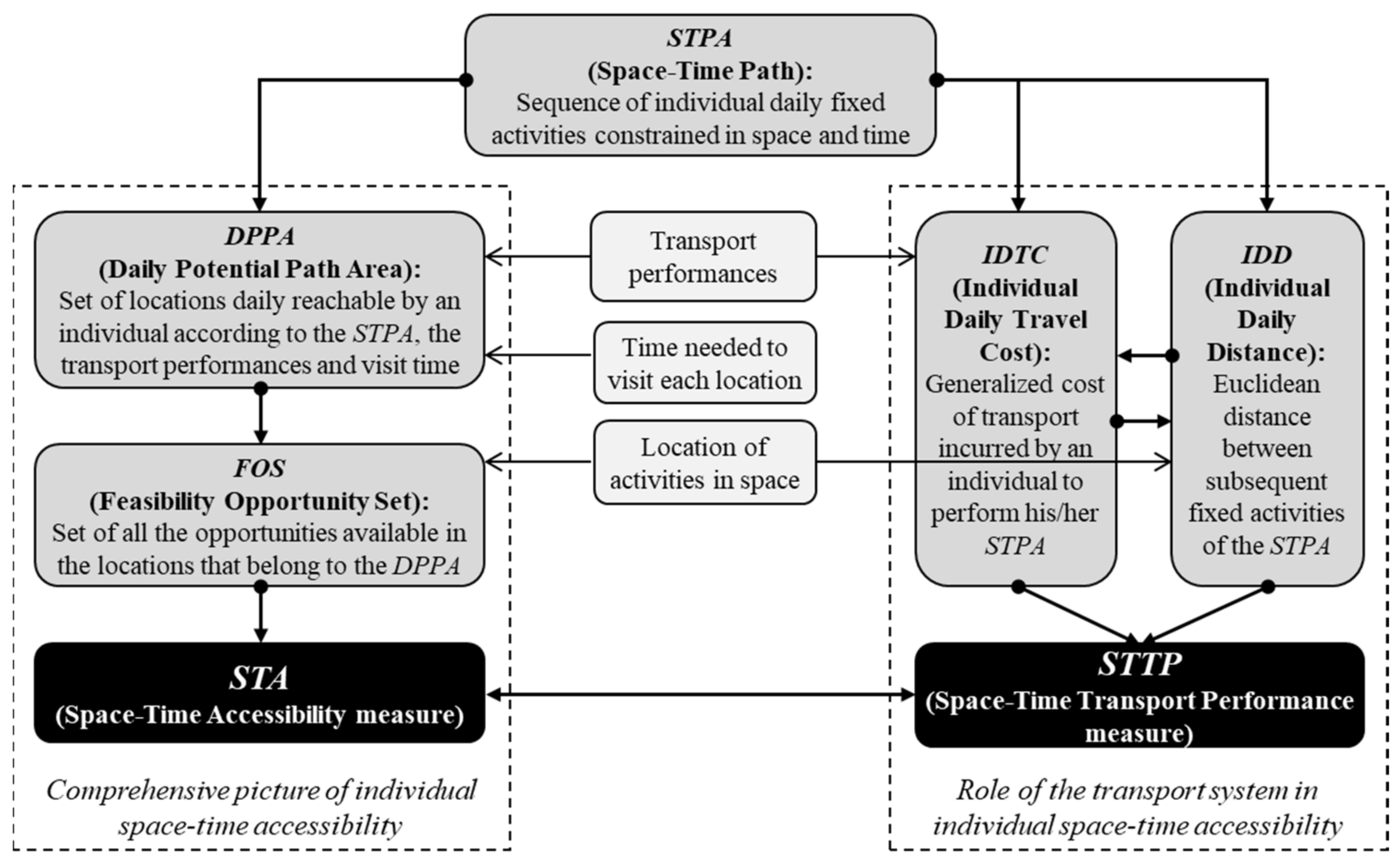
Figure 2.
Process for the computation of STPA (black), STA (red) and STTP (blue).
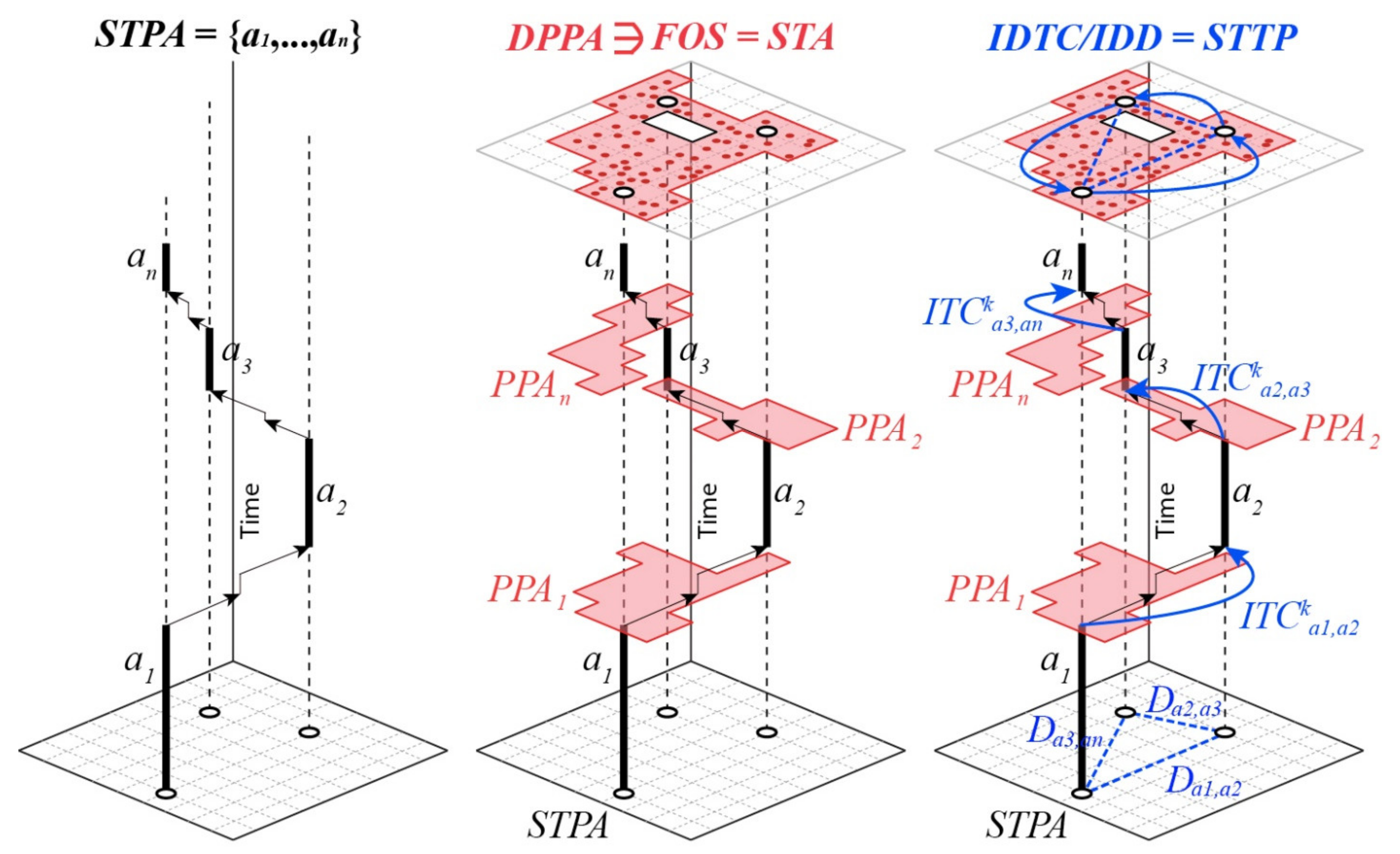
Figure 3.
Study area and key locations of the STPAs of the individuals A–E.
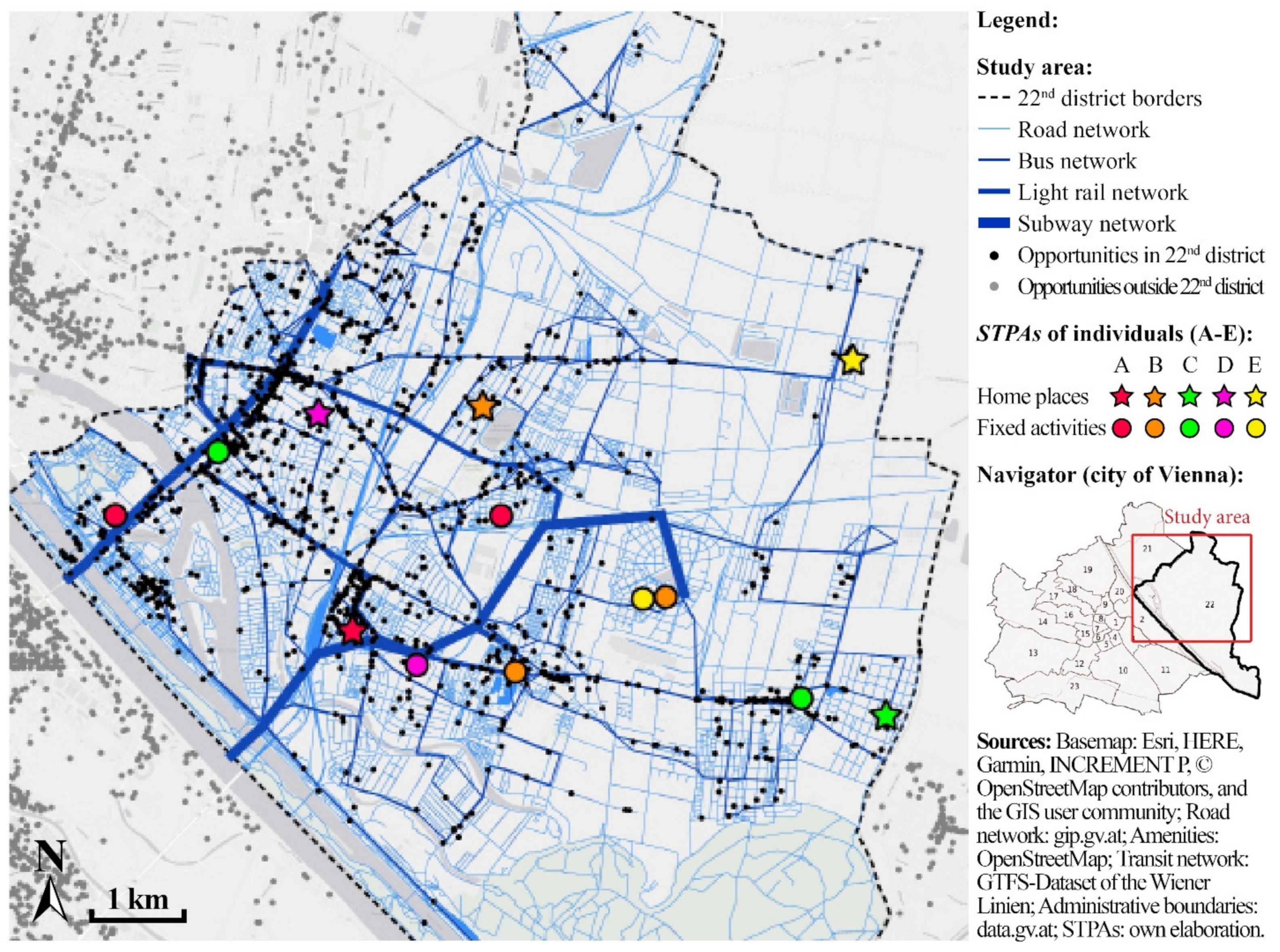
Figure 4.
Left, results of the STA computation; right, results of the STTP computation.

Table 2.
Exemplificative STPA to be set up for the calculation of STTP.
| Main STPAs Information | Fixed Activity a1 | Fixed Activity a2 | Fixed Activity a3 | Fixed Activity a4 | Fixed Activity a5 |
|---|---|---|---|---|---|
| Activity category: | Home-stay | Other | Work | Other | Home-stay |
| Activity location: | Street 1 | Street 2 | Street 3 | Street 2 | Street 1 |
| Activity timing: | 00:00–07:30 | 07:50–08:00 | 09:00–17:00 | 17:30–18:00 | 19:00–24:00 |
| Activity fixity degree: | 4 | 5 | 5 | 3 | 4 |
| * Transport mode(s): | - | Car driver | Car driver | Car driver | Car passenger |
* Notes: the transport mode used to reach the activity.
Table 3.
The STPAs of individuals A–E.
| Individuals | Main STPAs Information | STPAs of Indiviuals (A–E) | |||||||
|---|---|---|---|---|---|---|---|---|---|
| Fixed Activity a1 | Fixed Activity a2 | Fixed Activity a3 | Fixed Activity a4 | Fixed Activity a5 | Fixed Activity a6 | Fixed Activity a7 | Fixed Activity a8 | ||
| A | Activity category: | Home-stay | Other | Work | Home-stay | ||||
| Activity timing: | 00:00–07:30 | 07:40–07:45 | 08:00–17:30 | 18:00–24:00 | |||||
| Activity fixity degree: | 5 | 5 | 5 | 4 | |||||
| Transport mode(s): | - | Car driver | Car driver | Car driver | |||||
| B | Activity category: | Home-stay | Work | Other | Home-stay | Home-stay | |||
| Activity timing: | 00:00–06:30 | 07:00–12:00 | 12:30–12:35 | 13:00–15:00 | 17:30–24:00 | ||||
| Activity fixity degree: | 5 | 5 | 5 | 4 | 3 | ||||
| Transport mode(s): | - | Car driver | Car driver | Car driver | PT, Walking | ||||
| C | Activity category: | Home-stay | Other | Home-stay | Home-stay | Other | Home-stay | Work | Home-stay |
| Activity timing: | 00:00–07:25 | 07:45–07:50 | 08:20–09:30 | 12:00–14:00 | 14:15–14:20 | 14:35–17:00 | 18:00–23:00 | 24:00–24:00 | |
| Activity fixity degree: | 4 | 5 | 3 | 4 | 5 | 4 | 5 | 5 | |
| Transport mode(s): | - | Walkig | Walking | PT, Walking | Walking | Walking | PT | PT | |
| D | Activity category: | Home-stay | Other | Home-stay | Home-stay | ||||
| Activity timing: | 00:00–09:00 | 10:00–11:30 | 13:00–15:00 | 18:00–24:00 | |||||
| Activity fixity degree: | 4 | 5 | 4 | 3 | |||||
| Transport mode(s): | - | PT | PT | PT, Walking | |||||
| E | Activity category: | Home-stay | Education | Home-stay | Home-stay | ||||
| Activity timing: | 00:00–07:30 | 08:00–14:00 | 15:00–18:00 | 20:00–24:00 | |||||
| Activity fixity degree: | 5 | 5 | 4 | 4 | |||||
| Transport mode(s): | - | Car passenger | PT | PT, Walking | |||||
Notes: Activity category: We define four activity categories: Home-stay, Work, Education, and Other. For individuals B–E, two consecutive home-stays occur in their STPAs. This is because they have two consecutive mandatory activities to perform at home and a free-time span in between to potentially engage in discretionary activities. Activity timing: This indicates the starting and ending time of each activity. The first and last activities always start at 00:00 and end at 24:00. Activity fixity degree: 1–5 Likert scale, with 1 indicating maxium flexibility and 5 maximum fixity. Transport mode: This indicates the transport mode(s) used to reach the related activity. We define four transport modes: Car driver, Car passenger, PT, and Walking. Since the first activity is always the early-morning home-stay, there is no transport mode assigned to reach it.
Table 4.
VTT values applied to the different modes of transport and categories of individuals.
| Categories | Full-Time Workers | Part-Time Workers | Pensioners | Pupils |
|---|---|---|---|---|
| Related individuals of the test | A | B and C | D | E |
| Hourly wage rate | €16.22/h | €13.78/h | €8.89/h | €9.88/h |
| VTT for car drivers | €9.73/h | €8.27/h | €5.33/h | €5.93/h |
| VTT for car and PT passenger | €7.30/h | €6.20/h | €4.00/h | €4.45/h |
| VTT for out-of-vehicle travel time | €16.22/h | €13.78/h | €8.89/h | €9.88/h |
Table 5.
Components for the calculation of STA and STTP for individuals A–E.
| Individuals | STPA | STA | STTP | |||||||||
|---|---|---|---|---|---|---|---|---|---|---|---|---|
| Subsequent Fixed Activities | Time Span * | Mode(s) of Transport | tta,a+1 | PPA | Ow∈ PPA | VTT | UMC | ICTka,a+1 | Da,a+1 | |||
| Cmka,a+1 | Civttka,a+1 | Covttka,a+1 | ||||||||||
| - | Min. | - | Min. | km2 | Num. | €/h | €/km | € | € | € | km | |
| A | a1→a2 | 15 | Car driver | 5 | 0.88 | 119 | 9.73 | 0.42 | 1.42 | 0.74 | 0.00 | 2.30 |
| a2→a3 | 15 | Car driver | 7 | 0 † | 0 † | 9.73 | 0.42 | 2.41 | 1.18 | 0.00 | 4.64 | |
| a3→a4 | 30 | Car driver | 5 | 6.32 | 779 | 9.73 | 0.42 | 1.81 | 0.86 | 0.00 | 3.16 | |
| B | a1→a2 | 30 | Car driver | 9 | 4.08 | 82 | 8.27 | 0.42 | 2.12 | 1.21 | 0.00 | 3.16 |
| a2→a3 | 30 | Car driver | 6 | 3.64 | 104 | 8.27 | 0.42 | 1.68 | 0.94 | 0.00 | 1.98 | |
| a3→a4 | 30 | Car driver | 7 | 6.24 | 357 | 8.27 | 0.42 | 2.12 | 0.84 | 0.00 | 3.17 | |
| a4→a5** | 150 | PT, Walking | 45 | 70.56 | 8924 | - | - | - | - | - | - | |
| C | a1→a2 | 20 | Walking | 9 | 0.32 | 1 | 13.78 | 0.00 | 0.00 | 0.00 | 2.09 | 0.52 |
| a2→a3 | 30 | Walking | 9 | 0.32 | 1 | 13.78 | 0.00 | 0.00 | 0.00 | 2.09 | 0.52 | |
| a3→a4** | 150 | PT, Walking | 45 | 39.16 | 1227 | - | - | - | - | - | - | |
| a4→a5 | 15 | Walking | 9 | 0.32 | 1 | 13.78 | 0.00 | 0.00 | 0.00 | 2.09 | 0.52 | |
| a5→a6 | 15 | Walking | 9 | 0.32 | 1 | 13.78 | 0.00 | 0.00 | 0.00 | 2.09 | 0.52 | |
| a6→a7 | 60 | PT | 43 | 2.32 | 373 | 6.20 | 1.00 *** | 0.50 | 3.20 | 2.85 | 8.45 | |
| a7→a8 | 60 | PT | 39 | 2.32 | 373 | 6.20 | 1.00 *** | 0.50 | 3.00 | 2.36 | 8.45 | |
| D | a1→a2 | 60 | PT | 27 | 3.52 | 259 | 4.00 | 0.64 *** | 0.32 | 1.07 | 1.60 | 3.23 |
| a2→a3 | 90 | PT | 29 | 6.92 | 616 | 4.00 | 0.64 *** | 0.32 | 1.27 | 1.47 | 3.23 | |
| a3→a4** | 180 | PT, Walking | 60 | 186.68 | 29,892 | - | - | - | - | - | - | |
| E | a1→a2 | 30 | Car passenger | 9 | 7.44 | 101 | 4.45 | 0.42 | 0.00 | 0.70 | 0.00 | 3.78 |
| a2→a3 | 60 | PT | 34 | 1.84 | 30 | 4.45 | 0.21 *** | 0.21 | 0.74 | 3.90 | 3.78 | |
| a3→a4** | 120 | PT, Walking | 30 | 20.16 | 279 | - | - | - | - | - | - | |
Notes: * The time span between the ending time of a fixed activity and the starting time of the following one. ** Subsequent fixed activities occurring at the same location (i.e., home place) with a free-time span in between. Travels that could be potentially performed between them are considered in the STA computation, but not in the STTP one. *** For the values regarding PT, the unit of measure is €/day and not €/km. † PPA and Ow are equal to 0 because there is less than 10 min at disposal to engage in discretionary activities.
Table 6.
Results of STA and STTP for individuals A–E.
| Individuals | Time, Space and Transport Variables | STA | STTP | ||||||||||
|---|---|---|---|---|---|---|---|---|---|---|---|---|---|
| CT | OD | AS | AKC | ATC | DE | PMT | STA | rSTA | CV | STTP | rSTTP | CV | |
| h/day | n./km2 | km/h | €/km | €/min | % | Preferred mode(s) of transport | - | % | % | €/km | % | % | |
| A | 23 | 120.4 | 47 | 0.42 | 0.16 | 133 | Car driver | 800 | 2.68 | 153 | 0.83 | 88.09 | 19 |
| B | 20 | 125.7 | 42 | 0.42 | 0.14 | 182 | Car driver | 8947 | 29.93 | 1.07 | 68.48 | ||
| C | 18 | 31.3 | 11 | 0.05 | 0.18 | 114 | PT, Walking | 1227 | 4.10 | 1.20 | 61.21 | ||
| D | 18.5 | 160.1 | 9 | 0.08 | 0.10 | 127 | PT | 29,892 | 100.00 | 0.94 | 78.46 | ||
| E | 20 | 14.9 | 17 | 0.02 | 0.12 | 161 | Car passenger, PT | 330 | 1.10 | 0.73 | 100.00 | ||
Publisher’s Note: MDPI stays neutral with regard to jurisdictional claims in published maps and institutional affiliations. |
© 2022 by the authors. Licensee MDPI, Basel, Switzerland. This article is an open access article distributed under the terms and conditions of the Creative Commons Attribution (CC BY) license (https://creativecommons.org/licenses/by/4.0/).
Share and Cite
MDPI and ACS Style
Dianin, A.; Gidam, M.; Hauger, G. Isolating the Role of the Transport System in Individual Accessibility Differences: A Space-Time Transport Performance Measure. Appl. Sci. 2022, 12, 3309. https://doi.org/10.3390/app12073309
AMA Style
Dianin A, Gidam M, Hauger G. Isolating the Role of the Transport System in Individual Accessibility Differences: A Space-Time Transport Performance Measure. Applied Sciences. 2022; 12(7):3309. https://doi.org/10.3390/app12073309
Chicago/Turabian StyleDianin, Alberto, Michael Gidam, and Georg Hauger. 2022. "Isolating the Role of the Transport System in Individual Accessibility Differences: A Space-Time Transport Performance Measure" Applied Sciences 12, no. 7: 3309. https://doi.org/10.3390/app12073309
Note that from the first issue of 2016, this journal uses article numbers instead of page numbers. See further details here.