Exploring Microscopic Characteristics of Bicycle Riders’ following Behaviors in a Single-File Movement

Abstract

Cycling can bring a wide range of social, economic, and health benefits to individuals and communities. The safety and efficiency of bicycle facilities can be significantly impacted by the interactions among riders. This study aims to examine the microscopic characteristics of how cyclists interact with each other when they are in a single file movement based on the trajectory data collected from an experiment. Reaction delay was obtained by optimizing the correlation between relative speed and acceleration curves for individual cyclists and it was found that even for a given cyclist, this characteristic time delay could vary considerably, and be situation-dependent. Furthermore, it was found that the distribution of reaction delay, which has an average (±SD) of 0.66 s (±0.33 s), followed a log-normal distribution. The strong correlation observed between relative speed and time-delayed acceleration resembles the behavior observed in car-following situations, highlighting that relative speed is an essential factor influencing the acceleration behavior of cyclists. Multiple linear regression models were used to understand the association between acceleration and other key microscopic variables, e.g., spacing and relative speed, which are commonly used in microscopic behavior models. While the spacing between cyclists was found to have a significant impact on acceleration behavior, its effect was not as significant as that of relative speed. The outcomes of this study provide valuable insights into the cyclists’ behavior and can aid in the development of microscopic simulation models.

1. Introduction

Cycling has the potential to generate a diverse array of advantages for both individuals and communities, including benefits relating to social connections, economic growth, and physical well-being. Cycling can be considered as a cost-effective travel mode, particularly for short distance trips, which can save peoples’ money on fuel and parking costs. Bicycles, as well as other micromobility modes, can help to reduce traffic congestion by reducing the number of cars used for short distance trips [1,2,3,4]. Cycling is a low-impact form of exercise that can improve cardiovascular health [5]. Other health-related benefits include the reduction in local air pollution as a result of vehicle emissions, increase in physical activity, reduction in fatalities due to road crashes, reduction of stress, and promotion of mental health and well-being [6,7,8]. Overall, cycling can bring numerous benefits to individuals and communities, and can play an important role in promoting sustainable, healthy, and livable cities.

In addition to safety, the efficiency of bicycle infrastructure should also be evaluated in terms of traffic flow and capacity. Interactions between bicycle riders could largely influence the safety and efficiency of bicycle facilities. Microscopic simulation models could be used to investigate rider behavior; however, interactions between riders must be thoroughly studied in order to develop, calibrate, and validate such microscopic behavior models. To capture the microscopic behaviors of cyclists, several previous studies have developed, modified, and calibrated microscopic behavior models. Andresen et al. [9] calibrated a car-following model called the Necessary Deceleration Model (NDM) for bicycle traffic and explained that the NDM can realistically model the free acceleration of a cyclist and the behavior of cyclists moving in a group. Qu et al. [10] developed a microscopic model based on the social force model by Helbing and Molnar [11] to simulate the mixed traffic flows of electric bikes and cars. The force components of this model first considered the movement mechanisms and behaviors of electric bikes and cars separately. Then, the social force model was modified to consider the interactions between cars and electric bikes. Empirical data have been used to re-calibrate the parameters of the original social force model. Using trajectory data extracted from a single-file bicycle experiment, Xue et al. [12] calibrated five car-following models to explore cyclists’ following behaviors. The outcomes of this study explained that simple models, e.g., the velocity-based distance model (VDM), are adequate to realistically capture the cyclists’ following behaviors. Furthermore, they explained that the VDM bicycle-following model performs more or less the same as the NDM model as far as performance is concerned. Kaths et al. [13] used the data collected through a simulator experiment to calibrate the Wiedemann 99 car-following model [14] for bicycles. The outcomes of their study showed that the Wiedemann’s model could also be used to simulate cyclists’ following behaviors. Using the trajectory data collected through a bicycle-following experiment, Kurtc and Treiber [15] calibrated the Intelligent Driver Model (IDM) [16] to explain cyclists’ following behaviors. This study showed that traffic shockwaves for bicycle traffic could be realistically reproduced through the IDM. Furthermore, they concluded that, for bicycle traffic, the prediction power of the IDM is better than that of the NDM. Using the Inverse Reinforcement Learning concept [17], the interactions between cyclists and pedestrians were modelled, e.g., following and overtaking behaviors, when they share the space. The comparison of the simulated and actual trajectories explained that the model predicts the cyclists’ speed more accurately than the position.

Rui et al. [18] enhanced the social force model to simulate bicycle flow in groups. Numerical simulations were conducted in this study considering shoulder groups and following groups. The results explained that the negative impacts of shoulder groups are higher as compared to following groups and, therefore, shoulder grouping should be prohibited. This study is purely based on numerical simulation and validation is needed using experimental or real-world observational data. Li et al. [19] also modified the social force model to simulate the interactions between bicycles and cars at mixed-traffic intersections under high density bicycle traffic conditions. In the modified model, they considered a dynamic boundary model to incorporate the lateral dispersion of cyclists and a behavior force model to model interactions. The behavior force model consisted of four behaviors, namely, free moving, following, overtaking, and merging. Bicycle trajectories obtained through observations at a signalized intersection have been used to calibrate this model and the simulation results indicated that the modified social force model performs better than the original social force model.

Guo et al. [20] proposed a heuristic-based model to simulate the interactions between pedestrians and cyclists in shared spaces. The model was calibrated using the experimental data collected under pedestrian–bicycle mixed traffic conditions. This model reproduced lane formation, which is a commonly observed self-organization phenomenon in pedestrian dynamics. Guo et al. [21] calibrated a model to simulate bicycle traffic on wide roads using the data collected from bicycle experiments conducted on 3-m-wide tracks. Free riding, following, and overtaking behaviors have been explored in this study. In the model, they considered the movement direction, which was based on the view angle range. Furthermore, three relaxation times to represent acceleration, deceleration, and turning behaviors were used in their model. The findings of this study explained that the model could realistically reproduce bicycle flow dynamics.

These previous studies explain how existing microscopic models, such as the social force model and car-following models, can be re-calibrated to simulate bicycle traffic. While gleaning insights from these previous studies, the current study will comprehensively investigate the microscopic behavioral characteristics of cyclists when they interact with other cyclists. That is, in addition to the behaviors identified in established models, interaction characteristics and behavioral rules will be derived from the empirical data.

The key objective of this study is to explore the microscopic characteristics of the interactions between cyclists when they are following each other in a single file movement. Such situations could often be observed on narrow bicycle lanes. In particular, the characteristics of the interactions between cyclists, e.g., spacing, speeds, and acceleration, will be quantitatively assessed in detail. A key hypothesis of the proposed study is that the acceleration (or deceleration) of the follower is determined by the spacing and relative speed between the following and the leading cyclists. The findings of this study will be useful in developing microscopic behavior models that can be used in designing and assessing bicycle infrastructure and in evaluating the level of service and safety of bike lanes.

The structure of this paper is as follows: Section 2 outlines the methodology, including a depiction of the data and microscopic variables, while Section 3 presents the results of this study. The paper concludes with a discussion and conclusions section.

2. Methods

2.1. Data

The data used in this study was obtained from the single-file cycling experiment carried out by Andresen et al. [9] on May, 2012, in Wuppertal, Germany, with 33 participants. Based on the total number of participants in the elliptical experiment circuit, the length of which was set to 86 m, different experiment scenarios were considered. The total number of riders, N, within the circuit ranged from 5 to 33 and these scenarios were named as N = 5, N = 7, N = 10, N = 15, N = 18, N = 20, and N = 33. The complete set of experiments was recorded on video and coordinates of the riders’ head positions were extracted at a rate of 25 frames per second. Further information regarding the experiment, e.g., setup, procedures, and sample, can be found in Andresen et al. [9]. Time–space diagrams for N = 15, N = 18, N = 20, and N = 33 scenarios are shown in Figure 1. Local interactions between some pairs of consecutive cyclists can be observed in higher density cases (i.e., N = 20 and N = 33 cases). It should be noted that the global patterns emerged from local interactions. Therefore, local interactions are more significant than global parameters, including global density and flow.

2.2. Extracted Microscopic Variables for Cyclists’ Riding Behaviors

When a single file movement is considered, microscopic behavior models, such as the social force model and car-following models, rely on the assumption that the acceleration of a cyclist is primarily influenced by their interaction with the cyclist in front of them. This means that the acceleration should show a significant correlation with spacing and relative speed between consecutive riders.

It is important to mention that the open-source data provided solely the x and y coordinates over time, but by analyzing this data, we were able to derive microscopic variables, such as spacing, speed, and acceleration, using the following equations. From individual trajectories, microscopic variables of the single-file bicycle flow are derived as follows:

$$s_{i,i+1}\left(t\right)=x_{i+1}\left(t\right)-x_i\left(t\right)$$

(1)

where $s_{i,i+1}\left(t\right)$ is the spacing between leading and following cyclists, $x_i\left(t\right)$ is the x-coordinate of the cyclist $i$’s position at time $t$, and $x_{i+1}\left(t\right)$ is the x-coordinate of the preceding cyclist $\left(i+1\right)$’s position at time $t$.

$$v_i\left(t\right)=\frac{x_i\left(t+∆t/2\right)-x_i\left(t-∆t/2\right)}{∆t}$$

(2)

where $v_i\left(t\right)$ denotes the instantaneous speed of the cyclist $i$ at time $t$, and $∆t$ is the sampling interval that was set as 0.4 s.

$$a_i\left(t\right)=\frac{v_i\left(t+∆t/2\right)-v_i\left(t-∆t/2\right)}{∆t}$$

(3)

where $a_i\left(t\right)$ denotes the instantaneous acceleration of the cyclist $i$ at time $t$.

2.3. Modelling Cyclists’ following Behaviors

Several previous studies, e.g., Xue et al. [12], Kurtc and Treiber [15], and Kaths et al. [13], described bicycle riders’ following behaviors using car-following models. Car-following behavior describes the action of the following vehicle, i.e., maintaining a safe distance by accelerating or decelerating, in response to the leading vehicle’s actions. The stimulus–response approach, which is the most common method in modelling car-following behavior, considers that the following car responds to a stimulus (a change in driving conditions) after a lapse of time, which is called the reaction time. The stimulus could be a change in spacing or relative speed, whereas the response is the acceleration or deceleration. Chandler et al. [22], which is one of the earliest car-following models, formulated the linear relationship between the acceleration of the following vehicle (response) and the relative speed (stimulus) as follows:

$$A_F\left(t+T\right)=\lambda \left[V_L\left(t\right)-V_F\left(t\right)\right]$$

(4)

where $A_F$ is the acceleration or deceleration of following vehicle, $V_L$ and $V_F$ are the speeds of the leading and following vehicles, respectively, $T$ is the reaction time, and $\lambda$ is a model parameter called the sensitivity factor.

Helly [23] considered a linear combination of the relative speed and spacing, and proposed another linear model as given in the following equation:

$$A_F\left(t+T\right)={\lambda }_v \left[V_L\left(t\right)-V_F\left(t\right)\right]+{\lambda }_l \left[X_L\left(t\right)-X_F\left(t\right)-D\left(t\right)\right]$$

(5)

where $X_L$ and $X_F$ are the locations of leading and following vehicles, respectively, at a given time $t$, $D\left(t\right)$ is the safety distance between vehicles, and ${\lambda }_v$ and ${\lambda }_l$ are model parameters.

Gazis et al. [24] introduced a non-linear model that is called the general motors model by incorporating spacing, relative speed, and the speed of the following vehicle. The functional form of this non-linear model is as follows:

$$A_F\left(t+T\right)=\lambda \frac{{\left[V_F\left(t\right)\right]}^m}{{\left[X_L\left(t\right)-X_F\left(t\right)\right]}^l} \left[V_L\left(t\right)-V_F\left(t\right)\right]$$

(6)

where $\lambda$, $m$, and $l$ are model parameters.

It can be noted that the car-following models use desired speed, relative speed, and spacing as key model parameters. Using car-following models, the current study describes the dynamic nature and instability characteristics of the microscopic following behaviors of bicycle riders.

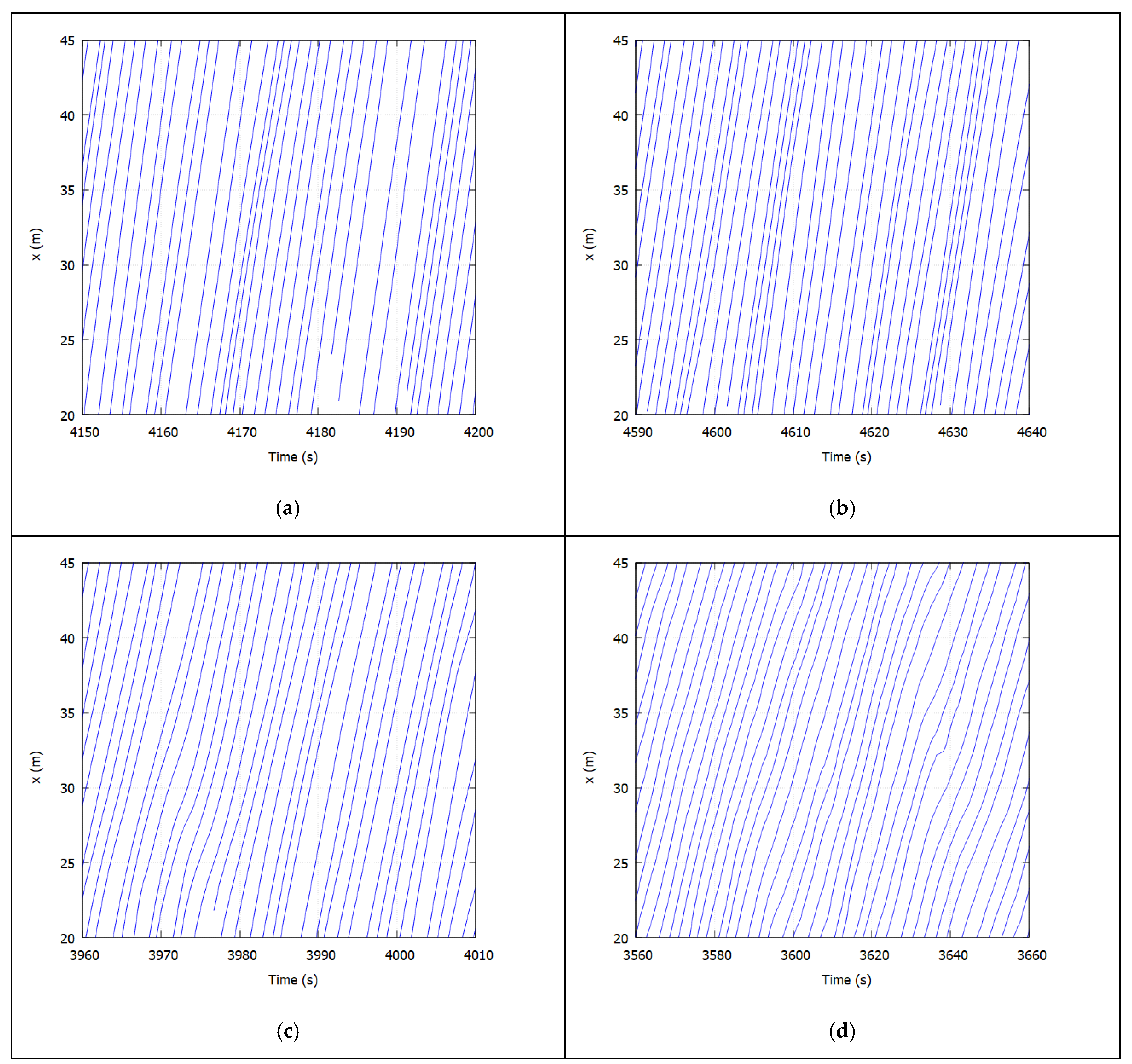
3. Characteristics of the Cyclists’ Interactions

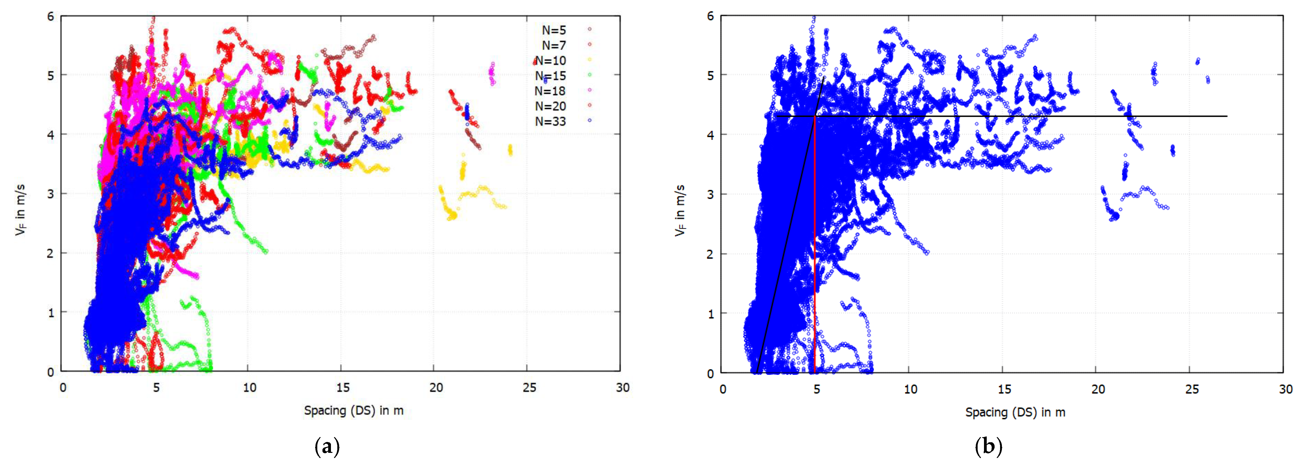
3.1. Relationship between Speed and Spacing

The relation between the speed of the following cyclist and the spacing between the leading and following cyclists for different global density levels is shown in Figure 2a.

Combining the linear relationship of the safety distance and the speed proposed by Andresen et al. [9], as well as the free-flow speed of the cyclists, i.e., 15.5 km/h (≈4.3 m/s), a piecewise linear relationship was obtained for the spacing and speed relationship as shown in Figure 2b. The linear relationship of the safety distance and the speed proposed by Andresen et al. [9] is given as:

$$DS=1.93+0.72 V_F$$

(7)

where $DS$ is the spacing between leading and following cyclists and $V_F$ is the speed of the following cyclist. From the piecewise linear relationship, it can be observed that, in general, speed is affected when the spacing is approximately less than 5 m. A similar single-file bicycle experiment conducted in China on a circular track with a circumference of 52 m reported approximately 4 m as the optimal spacing for 2.5 m/s free-flow speed (or desired speed) [25]. The explanation for these differences can be attributed to different experimental settings and the geometry of the track, e.g., the free-flow speed on a circular track is expected to be lower than on a straight track.

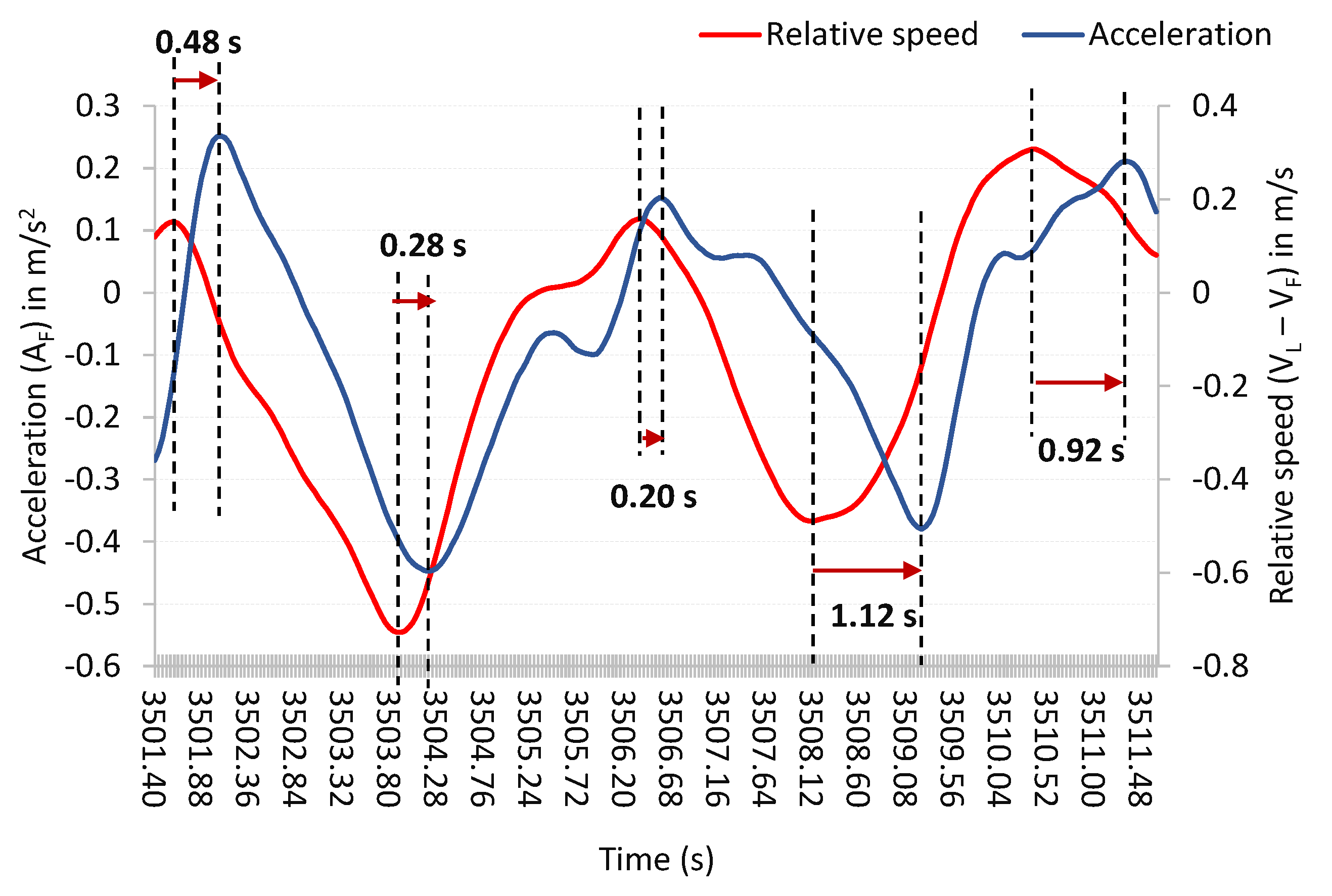
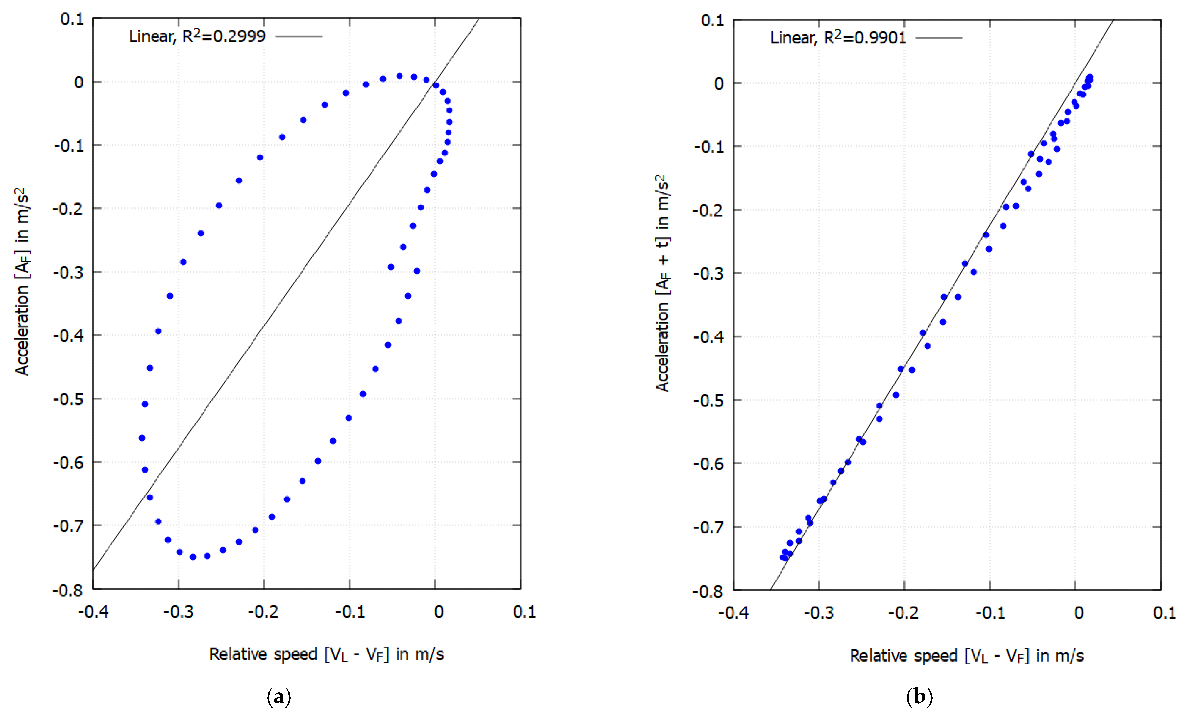
3.2. Relationship between Relative Speed and Acceleration

Using the time series of the acceleration of the following vehicle and the relative speed between the leading and following vehicles, Gurusinghe et al. [26] explored a graphical method to estimate the time varied reaction time of vehicles in car-following situations. The applicability of such methods (that were originally used in modelling car-following behaviors) are explored in our study to understand the cyclists’ following behaviors. Time series of the relative speed ($V_L$ − $V_F$) and acceleration of the following cyclist ($A_F$) for one pair of consecutive cyclists are depicted in Figure 3.

It can be observed that the following cyclist adjusts his or her acceleration in response to the relative speed between the leading and following cyclists following a reaction delay. Thus, Chandler’s model in Equation (4) in Section 2.3 can be illustrated graphically using this figure. It can further be noted that the reaction time (of the following cyclist) considerably varies over time. This observation indicates that the reaction delay is not a constant, even for a given cyclist, and it is rather situational.

The relative speed between the leading and following cyclists versus the acceleration of the following cyclist plots for a pair of leading and following cyclists are shown in Figure 4. This plot is known as the Lissajous diagram, and it reveals that introducing a time lag (t) for acceleration substantially enhances the correlation between relative speed and instantaneous acceleration. These diagrams are comparable to the acceleration versus relative speed patterns exhibited by drivers during car-following situations [26,27]. The Lissajous diagram provides a straightforward method for estimating the sensitivity parameter ($\lambda$) and reaction time of linear car-following models (e.g., Equations (4) and (5)). It should be noted that the existence of a series of reaction time or sensory motor delay values (as observed in Figure 3) indicates that there could be a range of Lissajous curves. As a result, there could be a range of model parameter sets for a given pair of interacting cyclists.

For each pair of interacting cyclists, relative speed versus acceleration plots were constructed and reaction delays were obtained by optimizing the correlation, as shown in Figure 4. Estimated time lags varied from 0.20 s to 2.20 s with an average (±standard deviation) of 0.66 s (±0.33 s). As specified in previous studies on car-following models, drivers react to the actions of the leading driver, e.g., braking, after a time lag, which is specified as the “reaction time” [28]. In studies involving pedestrians, the time lag is typically referred to as the “visual–motor delay” and is generally assumed to be around 0.40 s [29,30]. The study by Dias et al. [31] found that this characteristic time delay varies from 0.12 s to 0.68 s. However, a higher average delay time was reported by Xue et al. [32] for the correlation between the speeds of children pedestrian pairs, where the average delay time ranged from 0.75 to 0.84 s. For micromobility vehicles, such as the Segway, the reaction time can be incorporated depending on the situation, e.g., when following a pedestrian or a cyclist and during normal following or sudden brake situations [33]. Dias et al. [33] reported that the average reaction times (±SDs) of Segway riders were 0.50 s (±0.29 s) and 0.70 s (±0.44 s) when following a cyclist and a pedestrian, respectively, during sudden brake situations. It can be noted that the reaction delay estimated in the current study (0.66 s ± 0.33 s) is consistent with the reaction times estimated by Dias et al. [33] for Segway riders.

The Kolmogorov–Smirnov (K-S) test of normality was conducted on the natural logarithm (LN) values of the reaction delays. The test results revealed that the distribution of the time-varying reaction delay follows a log-normal function. The K-S test statistic (D) was 0.05437, and the p-value was 0.58813, which indicated that the data does not differ significantly from that which is normally distributed. The distribution of the reaction delay along with the fitted log-normal curve is shown in Figure 5 below. Figure 6 compares the theoretical log-normal cumulative probability distribution function with the empirical cumulative distribution function, which also revealed that the reaction delay can be fitted to a log-normal distribution.

Aggregated relative speed versus time delayed acceleration plots for interacting cyclist pairs in the N = 33 scenario are shown in Figure 7. It is apparent from the figure that acceleration generally increases as relative speed increases. This implies that individuals accelerate or decelerate more when the difference in speed between themselves and the leading cyclist is larger. Results of the Pearson correlation indicated that there is a significantly large positive relationship between time delayed acceleration and relative speed (r = 0.561, p < 0.001). It should be noted that the slope of the regression line shown in Figure 7 represents the average slope for the data for all individual cyclists used in the figure, and depending on the characteristics of the individuals, different values for the slope can be obtained. Nevertheless, this approach provided a way to simply and directly calibrate Chandler’s model [22], which is shown in Equation (4). As can be noted from Figure 7, the sensitivity parameter ($\lambda$) is 0.6709. As reported in Ranjitkar et al. [27], this value can vary from 1.5 to 2.5 for cars.

3.3. Multiple Linear Regression Model for Acceleration and Deceleration Behaviors

Acceleration, relative speed, and spacing data extracted from the cyclist trajectories in the N = 33 scenario for spacing values less than 5.0 m were used in developing the multiple linear regression models. Strongly interacting pairs of cyclists were observed in this case (see Figure 1d and Figure 2a). In order to eliminate the averaging effect of positive and negative acceleration values when considered together in a single regression model, two multiple linear regression models were developed separately for acceleration and deceleration behaviors. The model’s predictor variables included relative speed (=$V_L$ − $V_F$, i.e., speed of the leading bicyclist minus the speed of the following bicyclist) and spacing (DS). Time-delayed instantaneous acceleration and deceleration were the predicted variable. Due to its significant correlation with relative speed and spacing (see Figure 2), instantaneous speed was not entered as a predictor variable. The observations with standardized residuals greater than |3| can be considered outliers [34] and were, therefore, removed. Results of linear regression models for acceleration and deceleration behaviors are presented in the following sections.

3.3.1. Model for Acceleration Behavior

In this model, only positive instantaneous acceleration values and related other variables linked with positive acceleration events were taken into account. Only the acceleration behavior was investigated as a function of relative speed and spacing. The ANOVA results indicated that the acceleration behavior model was significant (

Table 1. Outcomes of the ANOVA test for the multiple linear regression models for acceleration behavior.

	Sum of Squares	df	Mean Square	F	Sig.
Regression	3.213	2	1.607	128.743	0.000
Residual	131.287	10,520	0.012
Total	134.500	10,522

). However, the r-squared value was 0.024, which is due to the higher scatter in the data. This higher scatter can be explained by the fact that we used the positions (x- and y-coordinates) of cyclists to calculate speed and acceleration. Nevertheless, according to the outcomes of the regression model, both relative speed and spacing were found to be significant predictors. Instantaneous acceleration showed a positive association with both relative speed ($V_L$ − $V_F$) and spacing (

Table 2. Coefficients in the multiple linear regression models for acceleration behavior.

	Coefficients		t	Sig.
	B	Std. Error
(Constant)	0.106	0.005	21.387	0.000
DV	0.086	0.006	15.010	0.000
DS	0.010	0.001	6.588	0.000

). This makes sense since cyclists tend to accelerate to catch up with the leading bicyclist if they are slower than the leading bicycle. Similarly, when there is more spacing in front of bicyclists, they are likely to accelerate.

3.3.2. Model for Deceleration Behavior

In this model, deceleration behavior was considered, and the negative values of instantaneous acceleration were taken into account. The ANOVA results indicated that the acceleration behavior model was significant (

Table 3. Outcomes of the ANOVA test for the multiple linear regression models for deceleration behavior.

	Sum of Squares	df	Mean Square	F	Sig.
Regression	8.058	2	4.029	262.675	0.000
Residual	162.319	10,582	0.015
Total	170.377	10,584

). The r-squared value was 0.047. As mentioned before, this low r-squared value may be due to the scatter of speed and acceleration data. Only relative speed ($V_L$ − $V_F$) was found to be a significant predictor (

Table 4. Coefficients in the multiple linear regression models for deceleration behavior.

	Coefficients		t	Sig.
	B	Std. Error
(Constant)	0.164	0.005	31.392	0.000
DS	−0.001	0.002	−0.741	0.458
DV	−0.123	0.005	−22.877	0.000

), having a negative association with deceleration behavior; thus, deceleration increased as relative speed decreases. That is, when the speed of the following bicyclist is higher than that of the leading bicyclist, the following cyclist is likely to decelerate to avoid a potential collision with the leading bicyclist

In this model, deceleration behavior was considered, i.e., the negative values of instantaneous acceleration were taken into account. The ANOVA results indicated that the acceleration behavior model was significant (Table 3). The r-squared value was 0.047. As mentioned before, this low r-squared value may be due to the scatter of speed and acceleration data. Only relative speed ($V_L$ − $V_F$) was found to be a significant predictor (Table 4), having a negative association with deceleration behavior; thus, deceleration increased as relative speed decreases. That is, when the speed of the following bicyclist is higher than that of the leading bicyclist, the following cyclist is likely to decelerate to avoid a potential collision with the leading bicyclist.

4. Discussion and Conclusions

The safety and efficiency of bicycle facilities can be greatly impacted by the interactions between cyclists. The behavior of each cyclist can have a significant impact on how they interact with others at a microscopic level, ultimately shaping the global patterns of motion. The behavior of riders may be studied using microscopic simulation models. In order to develop, calibrate, and validate microscopic behavior models, interactions between riders must be thoroughly studied. This study used the data collected from a controlled experiment to derive key microscopic variables of cyclists’ riding behaviors, such as spacing, speed, and acceleration, which are commonly employed in microscopic behavior models. Relationships between these microscopic variables were explored in detail to understand the microscopic characteristics of cyclists’ interactions when they are moving in a single file.

Results of the reaction delay analysis explained that resembling car-following behaviors, cyclists adjust their behaviors after a specific characteristic delay time that may be defined as the ‘reaction time’ or ‘sensory motor delay’. Such a parameter could be considered in microscopic simulation models to enhance the accuracy of such models. As reported in previous studies, the reaction time for cars generally varies between approximately 1.2 and 1.5 s [27,28,35]. It can be noted that, on average, these values are larger than the reaction times for bicycles estimated in this study. This is logical as cycling does not involve complex tasks, e.g., moving the leg from the accelerator to the brake paddle to press the brake, as in driving. Furthermore, under high density situation, riders are generally prepared to brake and stop or reduce the speed to avoid a potential collision. Previous studies on the simulation of bicycle traffic used larger values, e.g., 1.2 s, for the reaction time [12,15]. Apparently, such studies have not used microscopic calibration methods that involve the comparison of trajectories. Nevertheless, the estimated reaction times were consistent with the reaction times reported in previous studies for micromobility vehicles such as the Segway. For example, as mentioned in Dias et al. [33], the average reaction time when a Segway rider follows a cyclist can be 0.91 s (±0.35 s) and 0.50 s (±29 s) for general following and sudden brake conditions, respectively.

According to the results of the multiple linear regression models used to model cyclists’ time-delayed accelerations and decelerations as functions of relative speed and spacing, relative speed is a key predictor of the acceleration and deceleration behaviors of the cyclists. Spacing does not show a strong association; however, it was a significant predictor of the time delayed acceleration. In addition, relative speed and time delayed (by a reaction time) acceleration plots showed a strong correlation. These outcomes indicate that, with re-calibration, simple car-following models, e.g., Chandler’s model [22] and Helly’s model [23], can be used to simulate bicycle traffic on narrow bike paths. Xue et al. [12] also mentioned that complex models are not necessary and simpler models with a relatively smaller number of parameters are adequate to realistically capture cyclists’ following behaviors. However, the findings of the study of Xue et al. [12] mentioned that a velocity-based distance model, which mainly used the spacing between the following and leading cyclists, performed better than the speed matching model, which used speed difference and is equivalent to Chandler’s model [22]. It is important to note that there is a contradiction between this result and the findings of the current study. Stronger interactions, e.g., stop-and-go waves, were observed in the data used in [12] as compared to the current study. Experiment conditions might play a role in such differences and additional data, e.g., real world observations, might be necessary to verify such concerns. In addition, higher fluctuations can be expected in following situations under high-density conditions [36].

The study has some limitations, which need to be taken into consideration. Firstly, this study used a limited sample, and the data was collected in a controlled experiment only for a single-file movement. Therefore, the findings may not be applicable to more complex scenarios involving different cycling formations, e.g., several lines of cyclists on one-way paths, two-way paths, or wider paths. Additionally, the study did not take into account the potential impact of demographic characteristics on cyclists’ behaviors. Further research is needed to understand how demographic factors, e.g., gender and age of the riders, influence the reactions and behaviors of the cyclists. Moreover, future studies could also consider other factors such as wider paths, grades (upward/downward paths), bicycle size, road conditions, weather, time of the day, etc. Future studies could incorporate these factors as well as reaction times into simulation models to improve their accuracy and reliability.

References

1. Wang, M.; Zhou, X. Bike-sharing systems and congestion: Evidence from US cities. J. Transp. Geogr. 2017, 65, 147–154. [Google Scholar] [CrossRef]
2. Hamilton, T.L.; Wichman, C.J. Bicycle infrastructure and traffic congestion: Evidence from DC’s Capital Bikeshare. J. Environ. Econ. Manag. 2018, 87, 72–93. [Google Scholar] [CrossRef]
3. Fan, Y.; Zheng, S. Dockless bike sharing alleviates road congestion by complementing subway travel: Evidence from Beijing. Cities 2020, 107, 102895. [Google Scholar] [CrossRef]
4. Teixeira, J.F.; Silva, C.; Moura e Sá, F. Empirical evidence on the impacts of bikesharing: A literature review. Transp. Rev. 2021, 41, 329–351. [Google Scholar] [CrossRef]
5. Grøntved, A.; Rasmussen, M.G.; Blond, K.; Østergaard, L.; Andersen, Z.J.; Møller, N.C. Bicycling for transportation and recreation in cardiovascular disease prevention. Curr. Cardiovasc. Risk Rep. 2019, 13, 26. [Google Scholar] [CrossRef]
6. De Hartog, J.J.; Boogaard, H.; Nijland, H.; Hoek, G. Do the health benefits of cycling outweigh the risks? Environ. Health Perspect. 2010, 118, 1109–1116. [Google Scholar] [CrossRef]
7. Lindsay, G.; Macmillan, A.; Woodward, A. Moving urban trips from cars to bicycles: Impact on health and emissions. Aust. New Zealand J. Public Health 2011, 35, 54–60. [Google Scholar] [CrossRef] [PubMed]
8. Ma, L.; Ye, R.; Wang, H. Exploring the causal effects of bicycling for transportation on mental health. Transp. Res. Part D Transp. Environ. 2021, 93, 102773. [Google Scholar] [CrossRef]
9. Andresen, E.; Chraibi, M.; Seyfried, A.; Huber, F. Basic driving dynamics of cyclists. In Simulation of Urban MObility User Conference; Springer: Berlin/Heidelberg, Germany, 2013; pp. 18–32. [Google Scholar]
10. Qu, Z.W.; Cao, N.B.; Chen, Y.H.; Zhao, L.Y.; Bai, Q.W.; Luo, R.Q. Modeling electric bike–car mixed flow via social force model. Adv. Mech. Eng. 2017, 9, 1687814017719641. [Google Scholar] [CrossRef]
11. Helbing, D.; Molnar, P. Social force model for pedestrian dynamics. Phys. Rev. E 1995, 51, 4282. [Google Scholar] [CrossRef]
12. Xue, S.; Feliciani, C.; Shi, X.; Jiang, R. Understanding the single-file dynamics of bicycle traffic from the perspective of car-following models. J. Stat. Mech. Theory Exp. 2020, 2020, 053402. [Google Scholar] [CrossRef]
13. Kaths, H.; Keler, A.; Bogenberger, K. Calibrating the wiedemann 99 car-following model for bicycle traffic. Sustainability 2021, 13, 3487. [Google Scholar] [CrossRef]
14. Wiedemann, R. Simulation des Strassenverkehrsflusses; Schriftenreihe des Instituts für Verkehrswesen der Universität Karlsruhe, Band 8; Instituts für Verkehrswesen der Universität Karlsruhe: Karlsruhe, Germany, 1974. [Google Scholar]
15. Kurtc, V.; Treiber, M. Simulating bicycle traffic by the intelligent-driver model-Reproducing the traffic-wave characteristics observed in a bicycle-following experiment. J. Traffic Transp. Eng. (Engl. Ed.) 2020, 7, 19–29. [Google Scholar] [CrossRef]
16. Treiber, M.; Hennecke, A.; Helbing, D. Congested traffic states in empirical observations and microscopic simulations. Phys. Rev. E 2000, 62, 1805. [Google Scholar] [CrossRef] [PubMed]
17. Alsaleh, R.; Sayed, T. Modeling pedestrian-cyclist interactions in shared space using inverse reinforcement learning. Transp. Res. Part F Traffic Psychol. Behav. 2020, 70, 37–57. [Google Scholar] [CrossRef]
18. Rui, Y.X.; Tang, T.Q.; Zhang, J. An improved social force model for bicycle flow in groups. J. Adv. Transp. 2021, 2021, 2412655. [Google Scholar] [CrossRef]
19. Li, Y.; Ni, Y.; Sun, J. A modified social force model for high-density through bicycle flow at mixed-traffic intersections. Simul. Model. Pract. Theory 2021, 108, 102265. [Google Scholar] [CrossRef]
20. Guo, N.; Jiang, R.; Wong, S.C.; Hao, Q.Y.; Xue, S.Q.; Xiao, Y.; Wu, C.Y. Modeling the interactions of pedestrians and cyclists in mixed flow conditions in uni-and bidirectional flows on a shared pedestrian-cycle road. Transp. Res. Part B Methodol. 2020, 139, 259–284. [Google Scholar] [CrossRef]
21. Guo, N.; Jiang, R.; Wong, S.C.; Hao, Q.Y.; Xue, S.Q.; Hu, M.B. Bicycle flow dynamics on wide roads: Experiments and simulation. Transp. Res. Part C Emerg. Technol. 2021, 125, 103012. [Google Scholar] [CrossRef]
22. Chandler, R.E.; Herman, R.; Montroll, E.W. Traffic dynamics: Studies in car following. Oper. Res. 1958, 6, 165–184. [Google Scholar] [CrossRef]
23. Helly, W. Simulation of bottlenecks in single-lane traffic flow. In Proceedings of the Symposium on Theory of Traffic Flow, Research Laboratories, General Motors; Elsevier: Amsterdam, The Netherlands, 1959. [Google Scholar]
24. Gazis, D.C.; Herman, R.; Rothery, R.W. Nonlinear follow-the-leader models of traffic flow. Oper. Res. 1961, 9, 545–567. [Google Scholar] [CrossRef]
25. Zhao, Y.; Zhang, H.M. A unified follow-the-leader model for vehicle, bicycle and pedestrian traffic. Transp. Res. Part B Methodol. 2017, 105, 315–327. [Google Scholar] [CrossRef]
26. Gurusinghe, G.S.; Nakatsuji, T.; Azuta, Y.; Ranjitkar, P.; Tanaboriboon, Y. Multiple car-following data with real-time kinematic global positioning system. Transp. Res. Rec. 2002, 1802, 166–180. [Google Scholar] [CrossRef]
27. Ranjitkar, P.; Nakatsuji, T.; Azuta, Y.; Gurusinghe, G.S. Stability analysis based on instantaneous driving behavior using car-following data. Transp. Res. Rec. 2003, 1852, 140–151. [Google Scholar] [CrossRef]
28. Brackstone, M.; McDonald, M. Car-following: A historical review. Transp. Res. Part F Traffic Psychol. Behav. 1999, 2, 181–196. [Google Scholar] [CrossRef]
29. Le Runigo, C.; Benguigui, N.; Bardy, B.G. Visuo-motor delay, information–movement coupling, and expertise in ball sports. J. Sport Sci. 2010, 28, 327–337. [Google Scholar] [CrossRef]
30. Rio, K.W.; Rhea, C.K.; Warren, W.H. Follow the leader: Visual control of speed in pedestrian following. J. Vis. 2014, 14, 4. [Google Scholar] [CrossRef]
31. Dias, C.; Abdullah, M.; Ahmed, D.; Subaih, R. Pedestrians’ Microscopic Walking Dynamics in Single-File Movement: The Influence of Gender. Appl. Sci. 2022, 12, 9714. [Google Scholar] [CrossRef]
32. Xue, S.Q.; Shiwakoti, N.; Shi, X.M.; Xiao, Y. Investigating the characteristic delay time in the leader-follower behavior in children single-file movement. Chin. Phys. B 2022, 32, 028901. [Google Scholar] [CrossRef]
33. Dias, C.; Iryo, M.; Shimono, K.; Nakano, K. Experimental analysis of segway rider behavior under mixed traffic conditions. Seisan Kenkyu 2017, 69, 81–85. [Google Scholar]
34. Chow, L.F.; Zhao, F.; Liu, X.; Li, M.T.; Ubaka, I. Transit ridership model based on geographically weighted regression. Transp. Res. Rec. 2006, 1972, 105–114. [Google Scholar] [CrossRef]
35. Green, M.A. Roadway Human Factors: From Science to Application; Lawyers & Judges Publishing Company: Tucson, AZ, USA, 2018. [Google Scholar]
36. Roman, H.E.; Croccolo, F.; Riccardi, C. Extreme fluctuation events in a simple high-density traffic model. Phys. A Stat. Mech. Its Appl. 2008, 387, 5575–5582. [Google Scholar] [CrossRef]
Figure 1. Time–space diagrams for different global density levels (x represents the positions of cyclists). (a) N = 15; (b) N = 18; (c) N = 20; (d) N = 33.
Applsci 13 06539 g001
Figure 2. Spacing versus speed diagrams. (a) Spacing between leading and following cyclists versus speed of the following cyclist plots for different global density levels. (b) Aggregated spacing versus speed plot for all density levels and the piecewise linear relationship between them.
Applsci 13 06539 g002
Figure 3. Time-varying reaction time estimation based on time series of the relative speed between the leading and following cyclists and the acceleration of the following cyclist.
Applsci 13 06539 g003
Figure 4. Relative speed versus acceleration plots for a pair of leading (L) and following (F) cyclists. (a) Without a time lag. (b) With a time lag (t = 0.32 s).
Applsci 13 06539 g004
Figure 5. Distribution of the time varied reaction delay.
Applsci 13 06539 g005
Figure 6. Comparison of theoretical and empirical cumulative log-normal probability plots of the time varied reaction delay.
Applsci 13 06539 g006
Figure 7. Aggregated relative speed versus time-delayed acceleration plot with t = 0.66 s, which is the average value.
Applsci 13 06539 g007