

Multi-Point Displacement Synchronous Monitoring Method for Bridges Based on Computer Vision

College of Civil and Transportation Engineering, Shenzhen University, Shenzhen 518060, China
*
Author to whom correspondence should be addressed.
Appl. Sci. 2023, 13(11), 6544; https://doi.org/10.3390/app13116544
Submission received: 18 April 2023
/
Revised: 23 May 2023
/
Accepted: 24 May 2023
/
Published: 27 May 2023
(This article belongs to the Special Issue Advanced Structural Health Monitoring: From Theory to Applications II)
Abstract
:Bridge displacement is an important part of safety evaluations. Currently, bridge displacement monitoring uses only a few measurement points, making it difficult to evaluate safety. To address this problem, we propose a multi-point displacement synchronous monitoring method. The structural surface has abundant natural texture features, so we use the feature points of the structural surface as the displacement measurement points and propose a feature point displacement calculation method. Furthermore, we conduct experiments on a beam in the laboratory and obtain the beam’s multi-point displacement monitoring results. The monitoring results show that the displacement of some feature points is mismatched. We propose the use of the structural deflection curve to eliminate the feature point displacement mismatches. This method uses the maximum rotation angle of the deflection curve to eliminate displacement mismatches. The results indicate that it is effective to eliminate displacement mismatches in simple structures, such as simply supported beams. Finally, we obtain the test beam’s multi-point displacement synchronous monitoring results. Compared with the 3D laser scanning measurement method, the maximum error of the monitoring results is 8.70%. Research shows that the main reason for the monitoring error is image noise, and the noise interference problem due to its application in practical bridges requires further investigation. Compared with traditional displacement monitoring, this method has significant economic, efficiency, and data integrity advantages. The method has application prospects for multi-point displacement monitoring of simple structures, such as simply supported beams.
1. Introduction
In conventional bridge displacement monitoring, sensors are placed on the structure to obtain the structural response and conduct a safety evaluation. The number of monitoring points that can be arranged on the bridge is very limited, making it difficult to evaluate the bridge’s safety through the use of local monitoring point data.
With the development of computer technology and image acquisition equipment, the displacement monitoring method based on machine vision shows great development potential. This method obtains the monitoring results of the measuring points through feature point extraction, feature point recognition, and feature tracking of the structural image. This method has the outstanding advantages of simple installation, automation, and visualization, as well as being non-contact and having a low cost and high efficiency. Currently, it has become a research highlight in structural deformation monitoring.
As early as 1995, Stephen G.A. et al. [1] used the vision tracking system to measure the mid-span displacement of the Humber Bridge in the U.K. for the first time and compared it with the acceleration sensor. The results showed that visual technology was more suitable for low-frequency and large-displacement structural monitoring, and an accelerometer was more suitable for high-frequency and small-amplitude structural modal monitoring. In 1999, P Olaszek et al. [2] proposed applying the computer vision method to the deformation monitoring of railway bridges. They verified the feasibility of this method by monitoring the target point at the mid-span of the bridge. In 2003, D V J’auregui et al. [3] used close-range digital photography technology to monitor the vertical deflection of a bridge. They carried out a static load test on the bridge to prove the accuracy of their method.
With the further development of image monitoring technology, image-based structural displacement monitoring is no longer limited to single-point monitoring and image post-processing. Relevant research on multi-target and real-time measurements has gradually emerged. In 2006, J J Lee et al. [4] obtained the real-time displacement of a bridge on the basis of image monitoring technology and used the deformation information to evaluate its bearing capacity. The image monitoring information was used for a deeper structural analysis. In 2016, Dongming F et al. [5] used upsampled cross correlation (UCC) matching technology to measure the displacement of a three-story frame structure in the laboratory, obtained the displacement monitoring results of multi-point targets on the structure, and extracted the modal parameters of the structure. In 2016, Terán [6] et al. proposed a cross-correlation method to monitor the dynamic displacement of bridges. They collected video data of a pedestrian overpass through a camera and then obtained the displacement and modal information of the bridge using video amplification technology. In 2016, B. Pan et al. [7,8] combined the Digital Image Correlation (DIC) algorithm with photogrammetry technology to further develop a long-distance bridge deflection system. The system was successfully applied to multi-point deflection monitoring of the Wuhan Yangtze River Bridge.
Zhao X et al. [9,10] proposed a bridge displacement monitoring system based on laser projection, which can monitor multiple target points on the bridge at the same time. The application results from actual bridges showed that the system could accurately obtain the bridges’ dynamic and static displacement information. Liu P et al. [11,12] proposed a laser-based horizontal displacement monitoring method for foundation pits. They installed a laser transmitter at the monitoring point, projected the laser spot on the screen, and obtained the horizontal displacement of the monitoring point by shooting the change in the spot’s position with the camera. The stability, static, and displacement loading tests showed that the method had a high level of accuracy and met the engineering application requirements. It was determined that when monitoring multiple targets, it is necessary to reduce the camera’s tilt angle. In 2014, Ribeiro D et al. [13] proposed a dynamic displacement monitoring system for railway bridges based on video technology that automatically tracked target points on the basis of the RANSAC algorithm. The system comprised a camera, an optical lens, a lamp, and targets. The system successfully monitored five targets on a railway bridge for one year. In 2015, Feng M Q et al. [14] developed a structural displacement monitoring system based on machine vision, which could extract target displacement in real time from video images. They conducted experiments on two railway bridges and verified the system’s applicability to actual bridge monitoring by comparing it with displacement sensors. In 2017, Khuc T et al. [15] proposed a structural health monitoring system for structural displacement and vibration monitoring. The system used virtual objects to eliminate the dependence of machine vision on the target. The system used an improved feature point extraction algorithm to achieve vibration monitoring of a bridge without targets for the first time. In 2020, Lee J et al. [16] proposed a bridge displacement monitoring system using dual cameras for self-motion compensation. The main camera of the system monitored the main target fixed to the structure, and the sub-camera monitored the sub-targets arranged around the system to obtain the system’s motion parameters. Finally, the system compensated for the error caused by self-motion. They also verified the applicability of the system through indoor and on-site tests. In 2021, Kromanis R et al. [17] proposed a bridge monitoring method based on multi-camera positioning. This method required the positional relationships of multiple targets captured by different cameras to remain unchanged and then generated a pixel-size and length-size conversion matrix. The displacement of the structure could be calculated on the basis of the target images captured by cameras at any location. In 2020, Kim J et al. [18] proposed a structural displacement monitoring method based on camera motion compensation. This method combined image matching and feature detection algorithms to correct errors caused by camera motion. Compared with traditional methods, this method had the advantage of automatically correcting camera motion errors. They also successfully applied this method to the displacement monitoring of a bridge.
Computer vision was proposed in the 1950s and gradually entered the industrialization stage in the 1980s. At present, it has become a hot spot for Structural Health Monitoring (SHM) research. Computer vision has a high level of accuracy when used in structural displacement monitoring. It does not require professional technical personnel to operate, and it has outstanding advantages, such as simple equipment installation, a low equipment cost, and an efficient working performance. However, computer vision technology requires installation targets on bridges, and monitoring cameras can obtain only limited point displacement information. The displacement information of limited points cannot accurately reflect the safety status of the structure.
Therefore, we propose a multi-point displacement synchronous monitoring method. This method uses the SIFT algorithm in computer vision to generate feature points on the structural surface. These feature points are used as displacement measurement points, and calculating the displacement values of these feature points can obtain structural multi-point displacement monitoring results. This article combined the SIFT algorithm with structural displacement monitoring and obtained the structural multi-point displacement synchronous monitoring results for the first time, providing a new method for applying computer vision in structural deformation monitoring.
This study proposes a bridge multi-point displacement synchronous monitoring method, which can obtain multi-point displacement monitoring results of the structure by a single monitoring camera. The monitoring effect is similar to full-field displacement monitoring. This method can greatly expand the data on SHM and solve the problem of limited point monitoring leading to difficulty in evaluating the safety status of bridges.
2. Multi-Point Displacement Synchronous Monitoring Method
We used the Scale-invariant Feature Transform (SIFT) [19,20,21,22,23,24] algorithm to generate structural feature points. The SIFT algorithm decomposes the image into scale space and calculates extreme points in the scale space. These extreme points are detected after down-sampling and have obvious image features called feature points. Further, we calculate the gradient direction of each feature point and assign direction values to the feature points. Even if the object in the image undergoes displacement, the detected feature points can be matched through directional values. Therefore, the feature points extracted by the SIFT algorithm are invariant to scale, direction, and rotation. In addition, SIFT feature points are also stable to brightness change, affine transformation, and noise. The SIFT algorithm process is shown in Figure 1.
The structural surface has natural texture features, which can be extracted and matched using the SIFT algorithm before and after deformation. The extracted feature points can be used as measurement points for displacement monitoring. We placed the calibration board in two different positions and took photos. The extracted calibration board feature points are shown in Figure 2a, and the matching results of feature points are shown in Figure 2b. There are 2131 extracted feature points, and Figure 2a,b only presents the matching results of the first 9 feature points. The green line in Figure 2b is the matching line of feature points on the calibration board.
As shown in Figure 2b, the feature points on the calibration board at different positions can be matched using the SIFT algorithm. The structural surface has natural features, and the SIFT algorithm can extract these feature points. We used these feature points as monitoring points to achieve structural full-field displacement monitoring. As shown in Figure 3, we fixed the camera in front of the structure and captured two images, I1(x, y) and I2(x, y), before and after deformation. Due to the fixed camera, the same image coordinate system Oxy can be established before and after deformation. The coordinates of feature point A1 (Figure 3 red dot) extracted before deformation are A1(x1, y1), and the coordinates of its matching point after deformation are A′1(x′1, y′1). The vector formed by the feature points A1(x1, y1) and A′1(x′1, y′1) is the displacement D1. D1 has two parameters, length L1 and angle θ1. The calculation method for vector D1 is as follows:
D1 is the displacement of one point on the structural surface, and the displacement of all feature points on the structural surface is the set:
Set D comprises all Di, which is the initial calculation result of the structural multi-point displacement. Figure 4 shows the multi-point displacement calculation flowchart.
3. Structural Multi-Point Displacement Monitoring Test
We used a test beam to verify the above method. Figure 5 shows the beam’s dimensions and the material object.
3.1. Data Collection Equipment
In this experiment, we used a Fuji GFX-100 camera and Fuji GF 32–64/4 RLM WR lens to capture images of the beam. Table 1 shows the technical parameters of the camera and lens.
We placed the monitoring camera 7 m from the beam, facing the center of the beam. The position of the monitoring camera is shown in Figure 6.
We placed 13 dial indicators on the bottom of the beam to verify the test data. The arrangement of the dial indicators is shown in Figure 7.
We also validated the experimental data using a Leica P50 Scan-Station. For the validation test, we pasted code marks at the node of the test beam and compared the code marks’ displacement with the calculated displacement. The arrangement of the targets on the beam is shown in Figure 8a. The setup of the three-dimensional laser scanning validation test is shown in Figure 8b.
3.2. Loading of the Beam
We used mid-span loading to deform the test beam, as shown in Figure 9. We gradually loaded it from 0 kN to 400 kN in increments of 100 kN. We collected images and validation data of the beam for analysis under each load level.
3.3. Calibration Monitoring Resolution
We drew calibration lines on each vertical member of the beam, and the lengths L of the calibration lines were known, as shown in Figure 10. We calculated the number of pixels N for each calibration line in the image. By calculating L/N, we obtained the test’s monitoring resolution, as shown in Table 2.
We used the calibration results’ average value as the monitoring resolution. Then, after obtaining the pixel displacement of the beam, we calculated the actual displacement of the beam by using this monitoring resolution.
3.4. Initial Monitoring Results for the Beam’s Multi-Point Displacement
We captured the beam’s image, as shown in Figure 11a. The beam’s feature points extracted through the SIFT algorithm are shown in Figure 11b.
We only retained the feature points of the beam, as shown in Figure 12, and calculated the multi-point displacement using the above method. We found many mismatches in the initial calculation results due to the similarity of the natural textures on the beam’s surface. Due to the many mismatches, we only show the mismatches in the local areas of the experimental beam. The initial calculation results for the feature points at the red arrow position in Figure 12 are shown in Figure 13.
In Figure 13, the red and blue dots represent the feature points’ starting and ending positions, respectively. Figure 13 shows that most feature point displacements are almost parallel (green lines), which is consistent with the structural deformation. The directions and lengths of some displacement vectors are incorrect, as shown by the red lines in Figure 13.
This problem arose because the natural texture features of the bridge’s surface have a certain degree of similarity, increasing the difficulty of matching feature points and leading to some mismatches. Therefore, further study of the multi-point displacement mismatch elimination method is necessary.
4. A Method for Multi-Point Displacement Mismatch Elimination
4.1. The Beam’s Edge Deflection
We used the method presented in [25,26,27] to calculate the beam’s edge deflection. Mismatched feature points can be eliminated using the beam’s edge deflection. The test beam used in this test had four prominent edge extraction positions, as shown by the red circles in Figure 14a. We calculated the edge deflection at the bottom of the test beam for comparison with the dial indicator, as shown by the arrow in Figure 14a. We extracted the feature points at the beam’s bottom edge under various load levels to form deformation curves, as shown in Figure 14b.
It can be observed from Figure 14 that the extracted beam’s edge lines showed an obvious fluctuation effect, which was caused by the image noise. Figure 15a shows that the beam’s edge line exhibited similar distributions under different loads, and the crest and trough positions of the edge curve under different loads were similar. This is because, during the test, the light field environment in the laboratory is similar, and the noise distribution of the structural edge line has similarities under different load conditions, resulting in consistent fluctuations in the structural edge line under different loads. Based on this characteristic, the initial edge line (0 kN) can be deducted from the deformed edge line, thus reducing the influence of noise. The initial edge line (0 kN) was deduced from the beam’s edge line (under load levels 100–400 kN) to obtain the beam’s edge deflection curve. Figure 15b shows the beam’s edge deflection curve compared with the dial indicator.
Table 3 shows the extracted deflection values compared with the values measured by the dial indicator. The average error in the beam’s edge deflection was 2.17%, and the extracted beam’s deflection was consistent with the actual deformation.
4.2. Mismatch Elimination for Multi-Point Displacements
The deflection y and rotation angle are the two basic parameters of the displacement vector. The deflection y varies with the position of the section, and can be expressed as a continuous function. This is the deflection curve equation of the beam, and the inclination of its tangent is the section rotation angle . For small deformations, is very small, and the rotation angle equation can be expressed as:
Equation (4) can be used to solve the section rotation angle of the structural edge deflection (Figure 15b). Furthermore, the obtained section rotation angle can be the elimination condition for the multi-point displacement mismatch. Figure 16 shows the calculation results for the test beam’s edge rotation angle.
Figure 16 shows the test beam’s angle curve under load levels 100–400 kN. The angle curve provides a rotation constraint for the multi-point displacement. If the angle of the feature point’s displacement does not satisfy the angle curve, the displacement is considered a mismatch and can be eliminated. In addition to the angle curve elimination method, the beam’s edge deflection can be used for multi-point displacement mismatch elimination. The maximum deflection value of the edge line (Figure 15b) can eliminate the displacements with incorrect lengths. Figure 17 shows the method of displacement mismatch elimination through the rotation angle and deflection y.
The maximum rotation angle of the structure is at the ends of the beam, and the rotation angle values at the ends often differ. We selected the larger of these two rotation angle values as the threshold. Table 4 lists the extracted rotation angle thresholds under load conditions of 100–400 kN. Figure 18 shows the rotation angle threshold mismatch elimination process.
Special attention should be paid to checking whether the calculated multi-point displacement meets the deformation coordination of the structure after the feature point displacement mismatch is eliminated. If the multi-point displacement monitoring results of the structure show regularity, the monitoring results can be considered accurate. Suppose the monitoring result shows a sudden change in the displacement’s rotation angle in some areas and suddenly disappears. In that case, it is necessary to relax the rotation angle threshold to avoid the displacement rotation angle being greater than the rotation angle threshold due to some special conditions, such as structural damage leading to sudden changes in the rotation angle of displacement.
4.3. Elimination Results of the Beam’s Multi-Point Displacement Mismatches
Figure 19 shows the mismatch elimination processing results for the beam’s multi-point displacement.
It can be observed from Figure 19 that most of the mismatches were eliminated on the basis of the extracted beam’s deflection. All displacement lines were distributed in parallel after eliminating the mismatches, consistent with the structural deformation law. Therefore, the proposed method can effectively eliminate the multi-point displacement mismatches.
Figure 20 shows the beam’s multi-point displacement calculation results under each load condition obtained under the afore-mentioned method.
Figure 20 shows that the structural multi-point displacement synchronous monitoring method greatly enhances the monitoring data. The monitoring results are similar to the structural full-field displacement monitoring results.
5. Validation of the Monitoring Results
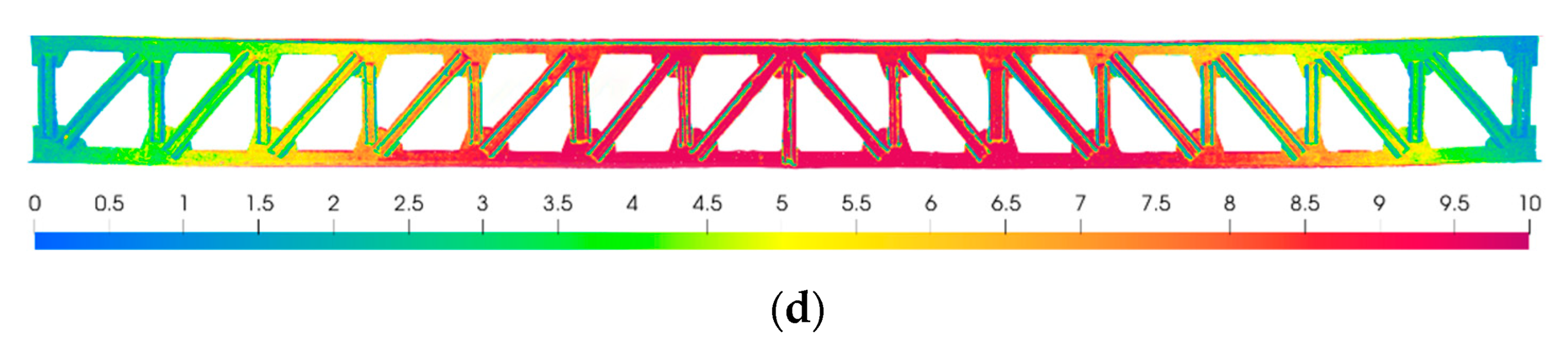
We used a Leica P50 Scan-Station to validate the monitoring results. The scanning accuracy is set to the highest, the scanning resolution is 0.3 mm/10 m, the target acquisition accuracy is 0.5 mm/50 m, and the noise accuracy is 0.2 mm/10 m. We obtained a three-dimensional model of the beam through three-dimensional laser scanning, as shown in Figure 21, and further obtained the deformation chromatograms of the beam model under various load conditions, as shown in Figure 22.
Using the pasted code marks on the beam, as previously shown in Figure 8a, we compared the displacement of the code marks’ positions in Figure 22 with those in Figure 20. The results are shown in Table 5, using a load condition of 400 kN as an example.
It can be observed from Table 5 that the displacement errors of the coded marks’ positions were within 9%, indicating that the calculated multi-point displacement can accurately reflect the structural displacement.
6. Conclusions
The structural health monitoring of bridges can be carried out to obtain data only at the local measuring points, and these incomplete measuring data lead to difficulties in evaluating the structural safety state. We proposed a structural multi-point synchronous monitoring method to solve this problem. The conclusions are as follows:
- The Scale-invariant Feature Transform (SIFT) algorithm can extract the structural feature points. These feature points can be used as measurement points for displacement monitoring. By establishing an image coordinate system, the displacement of feature points before and after deformation can be calculated.
- A 7 m long test beam was made in the laboratory. By drawing calibration lines on the vertical members of the test beam, the monitoring resolution of the image can be calculated. The monitoring resolution of the test beam image in this paper is 0.18 mm.
- The structural surface’s weak or repeated natural texture features can lead to the mismatches of some displacements. Hence, a displacement mismatch elimination method was proposed. This method uses the extracted deflection curve to constrain the displacement’s length and rotation angle. Hence, we achieved structural multi-point displacement mismatch elimination.
- We validated the test results using a three-dimensional laser scanning method. The maximum error of the monitoring results was 8.70%, and the average error was 4.21%. The monitoring results are consistent with the actual structural deformation.
- This method can expand the monitoring data. The monitoring results are similar to those of the structural full-field displacement monitoring and are expected to fundamentally solve the bridge safety evaluation problem of incomplete test data.
- This study yielded good monitoring results in the laboratory. However, the test beam’s image in the laboratory exhibits obvious noise, leading to the structural edge’s line shape undulation. The bridge environment is more complex than that of the laboratory, and the image noise is obvious. Therefore, the noise interference problem in the application of this method to practical actual bridges should be researched in future studies. It is recommended to use higher pixel hardware devices and more accurate feature point extraction algorithms in future studies to reduce the impact of noise.
- The multi-point displacement synchronous monitoring method of structures can be combined with structural damage identification. Compared to traditional single-point monitoring, multi-point displacement monitoring of structures can obtain more comprehensive monitoring data, and rotation angle information can be obtained through structural multi-point displacement. Whether the rotation angle can be used as a damage identification index combined with multi-point displacement monitoring methods still needs further research.
Author Contributions
X.C.: Conceptualization, Methodology, Investigation, Writing—Original draft preparation, Data curation, Writing—Review and Editing. Z.Z.: Conceptualization, Supervision, Project administration, Funding acquisition. W.Z.: Investigation, Data Curation, Validation, Software, Writing—Review and Editing. X.D.: Conceptualization, Methodology, Investigation, Writing—Review and Editing. All authors have read and agreed to the published version of the manuscript.
Funding
This work was supported by the Shenzhen Science and Technology Program No. JCYJ20220818095608018.
Institutional Review Board Statement
Not applicable.
Informed Consent Statement
Not applicable.
Data Availability Statement
Data will be made available on request.
Conflicts of Interest
The authors declare no conflict of interest.
References
- Stephen, G.A.; Brownjohn, J.M.W.; Taylor, C.A. Measurements of static and dynamic displacement from visual monitoring of the Humber Bridge. Eng. Struct. 1993, 15, 197–208. [Google Scholar] [CrossRef]
- Olaszek, P. Investigation of the dynamic characteristic of bridge structures using a computer vision method. Measurement 1999, 25, 227–236. [Google Scholar] [CrossRef]
- J´auregui, D.V.; White, K.R.; Woodward, C.B.; Leitch, K.R. Noncontact photogrammetric measurement of vertical bridge deflection. J. Bridge Eng. 2003, 8, 212–222. [Google Scholar] [CrossRef]
- Lee, J.J.; Cho, S.J.; Shinozuka, M.; Yun, C.B.; Lee, C.G.; Lee, W.T. Evaluation of bridge load carrying capacity based on dynamic displacement measurement using real–time image processing techniques. Int. J. Steel Struct. 2006, 6, 377–385. [Google Scholar]
- Dongming, F.; Feng, M.Q. Vision-based multipoint displacement measurement for structural health monitoring. Struct. Control. Health Monit. 2016, 23, 876–890. [Google Scholar]
- Terán, L.; Ordóñez, C.; García-Cortés, S.; Menéndez, A. Detection and magnification of bridge displacements using video images. Proc. Spie 2016, 151, 1015109. [Google Scholar]
- Pan, B.; Tian, L.; Song, X. Real-time, non-contact and targetless measurement of vertical deflection of bridges using off-axis digital image correlation. NDT E Int. 2016, 79, 73–80. [Google Scholar] [CrossRef]
- Long, T.; Pan, B. Remote Bridge Deflection Measurement Using an Advanced Video Deflectometer and Actively Illuminated LED Targets. Sensors 2016, 16, 1344. [Google Scholar]
- Zhao, X.; Liu, H.; Yu, Y.; Xu, X.; Hu, W.; Li, M.; Ou, J. Bridge Displacement Monitoring Method Based on Laser Projection-Sensing Technology. Sensors 2015, 15, 8444–8463. [Google Scholar] [CrossRef] [PubMed]
- Zhao, X.; Liu, H.; Yu, Y.; Zhu, Q.; Hu, W.; Li, M.; Ou, J. Displacement monitoring technique using a smartphone based on the laser projection-sensing method. Sens. Actuators A Phys. 2016, 246, 35–47. [Google Scholar] [CrossRef]
- Liu, P.; Liu, C.; Zhang, L.; Zhao, X. Displacement monitoring method based on laser projection to eliminate the effect of rotation angle. Adv. Struct. Eng. 2019, 22, 3319–3327. [Google Scholar] [CrossRef]
- Liu, P.; Xie, S.; Zhou, G.; Zhang, L.; Zhang, G.; Zhao, X. Horizontal displacement monitoring method of deep foundation pit based on laser image recognition technology. Rev. Sci. Instrum. 2018, 89, 125006. [Google Scholar] [CrossRef] [PubMed]
- Ribeiro, D.; Calçada, R.; Ferreira, J.; Martins, T. Non-contact measurement of the dynamic displacement of railway bridges using an advanced video-based system. Eng. Struct. 2014, 75, 164–180. [Google Scholar] [CrossRef]
- Feng, M.Q.; Fukuda, Y.; Feng, D.; Mizuta, M. Nontarget Vision Sensor for Remote Measurement of Bridge Dynamic Response. J. Bridge Eng. 2015, 20, 04015023. [Google Scholar] [CrossRef]
- Khuc, T.; Catbas, F.N. Completely contactless structural health monitoring of real-life structures using cameras and computer vision. Struct. Control Health Monit. 2017, 24, e1852. [Google Scholar] [CrossRef]
- Lee, J.; Lee, K.C.; Jeong, S.; Lee, Y.J.; Sim, S.H. Long-term displacement measurement of full-scale bridges using camera ego-motion compensation. Mech. Syst. Signal Process. 2020, 140, 106651. [Google Scholar] [CrossRef]
- Kromanis, R.; Kripakaran, P. A multiple camera position approach for accurate displacement measurement using computer vision. J. Civ. Struct. Health Monit. 2021, 11, 661–678. [Google Scholar] [CrossRef]
- Kim, J.; Jeong, Y.; Lee, H.; Yun, H. Marker-Based Structural Displacement Measurement Models with Camera Movement Error Correction Using Image Matching and Anomaly Detection. Sensors 2020, 20, 5676. [Google Scholar] [CrossRef]
- Xu, Y.; Brownjohn, J.M.W. Review of machine-vision based methodologies for displacement measurement in civil structures. J. Civ. Struct. Health Monit. 2018, 8, 91–110. [Google Scholar] [CrossRef]
- Spencer, B.F., Jr.; Hoskere, V.; Narazaki, Y. Advances in Computer Vision-Based Civil Infrastructure Inspection and Monitoring. Engineering 2019, 5, 199–222. [Google Scholar] [CrossRef]
- Zhang, L.; Liu, P.; Yan, X.; Zhao, X. Middle displacement monitoring of medium–small span bridges based on laser technology. Struct. Control Health Monit. 2020, 27, e2509. [Google Scholar] [CrossRef]
- Bai, X.; Yang, M.; Ajmera, B. An Advanced Edge-Detection Method for Noncontact Structural Displacement Monitoring. Sensors 2020, 20, 4941. [Google Scholar] [CrossRef]
- Yu, L.; Lubineau, G. A smartphone camera and built-in gyroscope based application for non-contact yet accurate off-axis structural displacement measurements. Measurement 2021, 167, 108449. [Google Scholar] [CrossRef]
- Lee, J.H.; Yoon, S.; Kim, B.; Gwon, G.H.; Kim, I.H.; Jung, H.J. A new image-quality evaluating and enhancing methodology for bridge inspection using an unmanned aerial vehicle. Smart Struct. Syst. 2021, 27, 209–226. [Google Scholar]
- Chu, X.; Zhou, Z.; Deng, G.; Duan, X.; Jiang, X. An Overall Deformation Monitoring Method of Structure Based on Tracking Deformation Contour. Appl. Sci. 2019, 9, 4532. [Google Scholar] [CrossRef]
- Deng, G.; Zhou, Z.; Shao, S.; Chu, X.; Jian, C. A Novel Dense Full-Field Displacement Monitoring Method Based on Image Sequences and Optical Flow Algorithm. Appl. Sci. 2020, 10, 2118. [Google Scholar] [CrossRef]
- Luo, R.; Zhou, Z.; Chu, X.; Liao, X.; Meng, J. Research on Damage Localization of Steel Truss–Concrete Composite Beam Based on Digital Orthoimage. Appl. Sci. 2022, 12, 3883. [Google Scholar] [CrossRef]
Figure 1.
SIFT algorithm process.
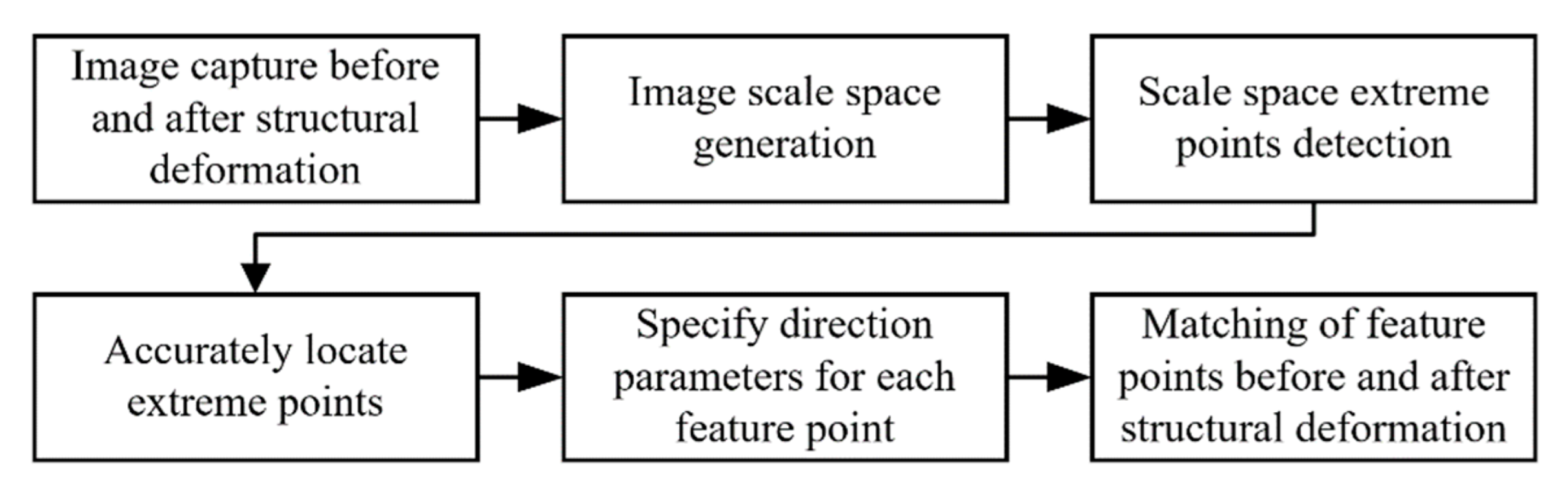
Figure 2.
Feature points extraction and matching results based on the SIFT algorithm. (a) Feature points on the calibration board. (b) Matching of feature points on calibration board at different positions.
Figure 2.
Feature points extraction and matching results based on the SIFT algorithm. (a) Feature points on the calibration board. (b) Matching of feature points on calibration board at different positions.

Figure 3.
Calculation method for structural multi-point displacement.
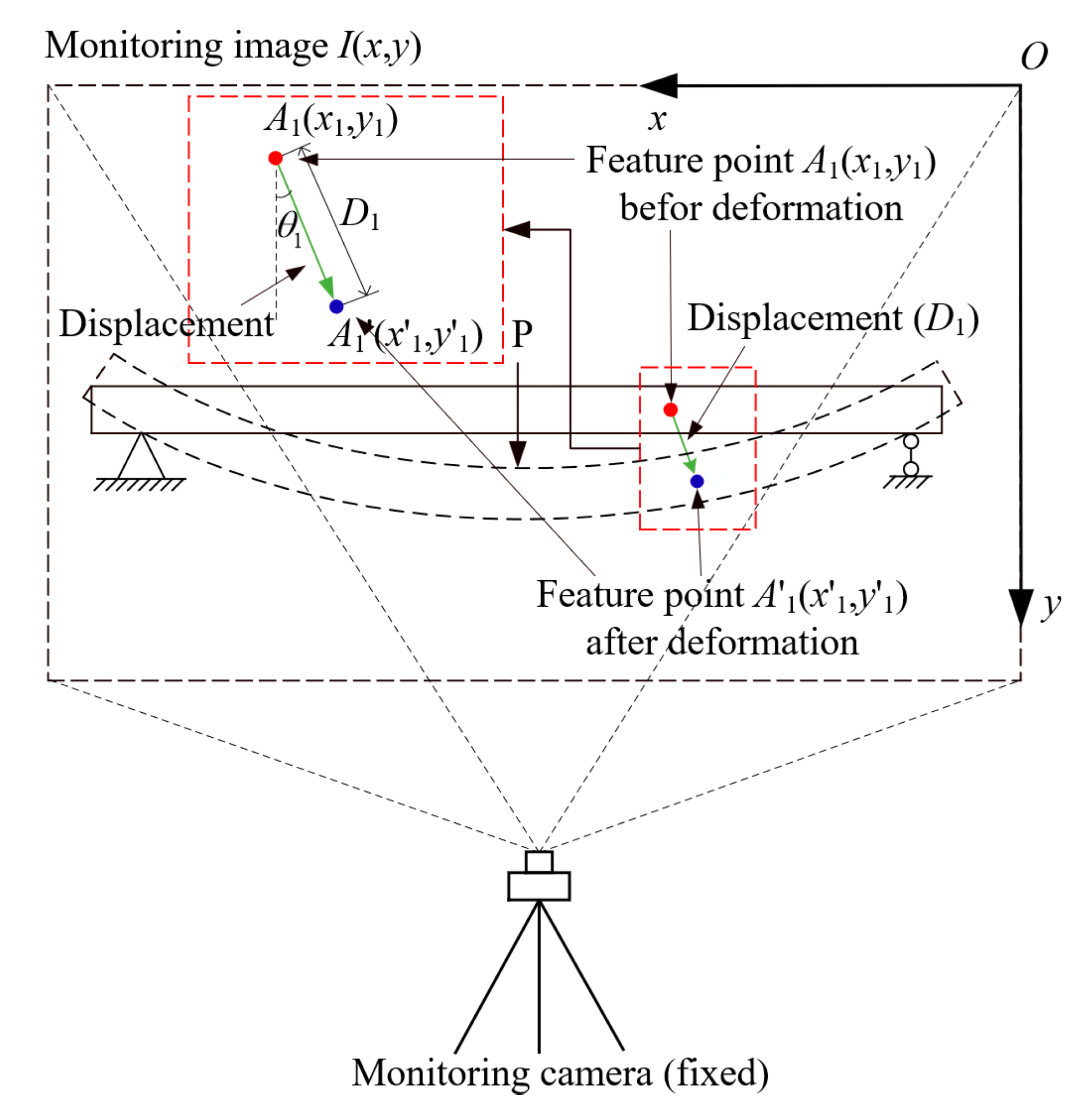
Figure 4.
Calculation flowchart of structural multi-point displacement.

Figure 5.
Dimensions and material object of the beam. (a) The beam’s dimensions (mm). (b) Material object of the beam.
Figure 5.
Dimensions and material object of the beam. (a) The beam’s dimensions (mm). (b) Material object of the beam.
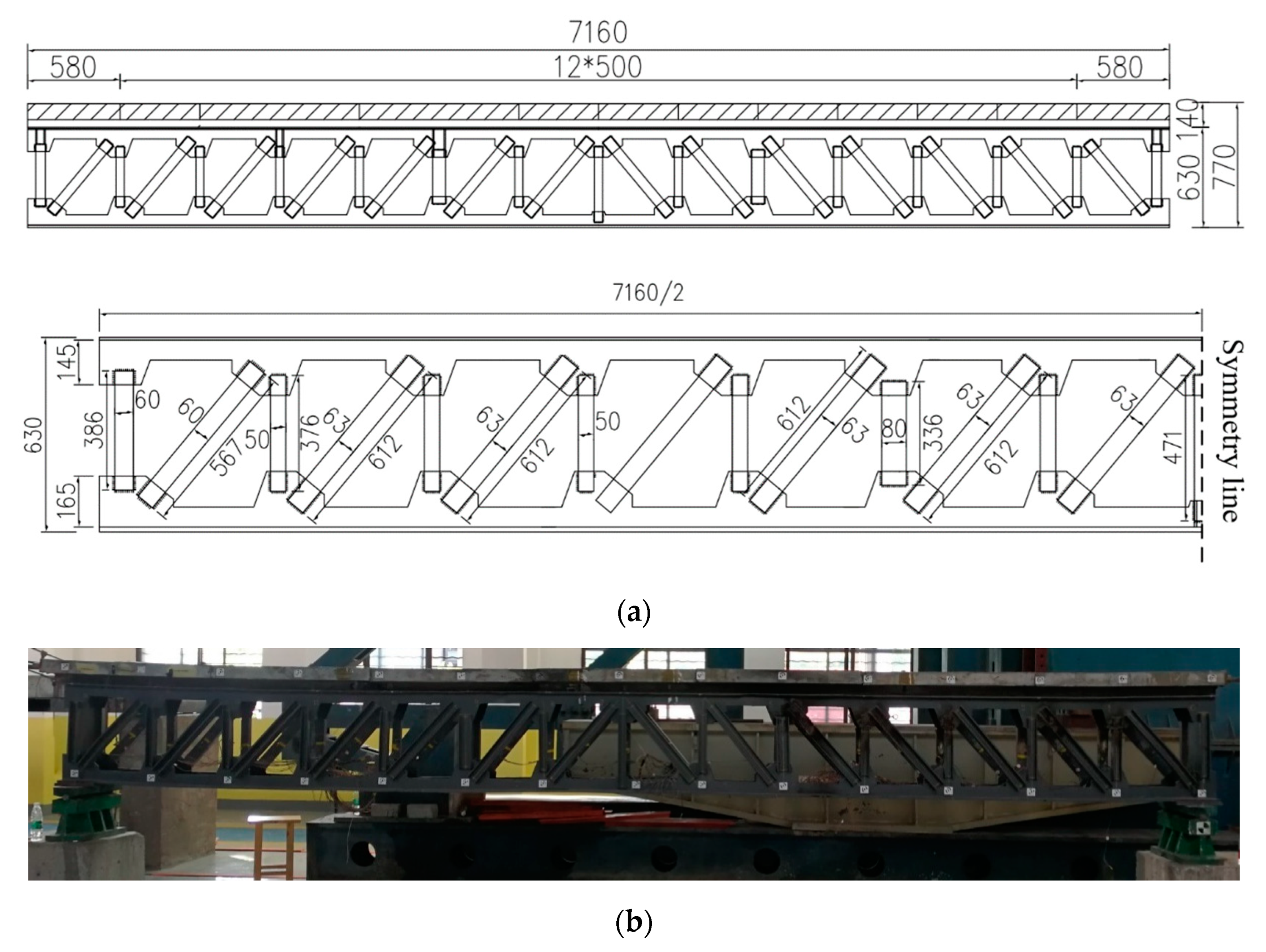
Figure 6.
Position of the monitoring camera.
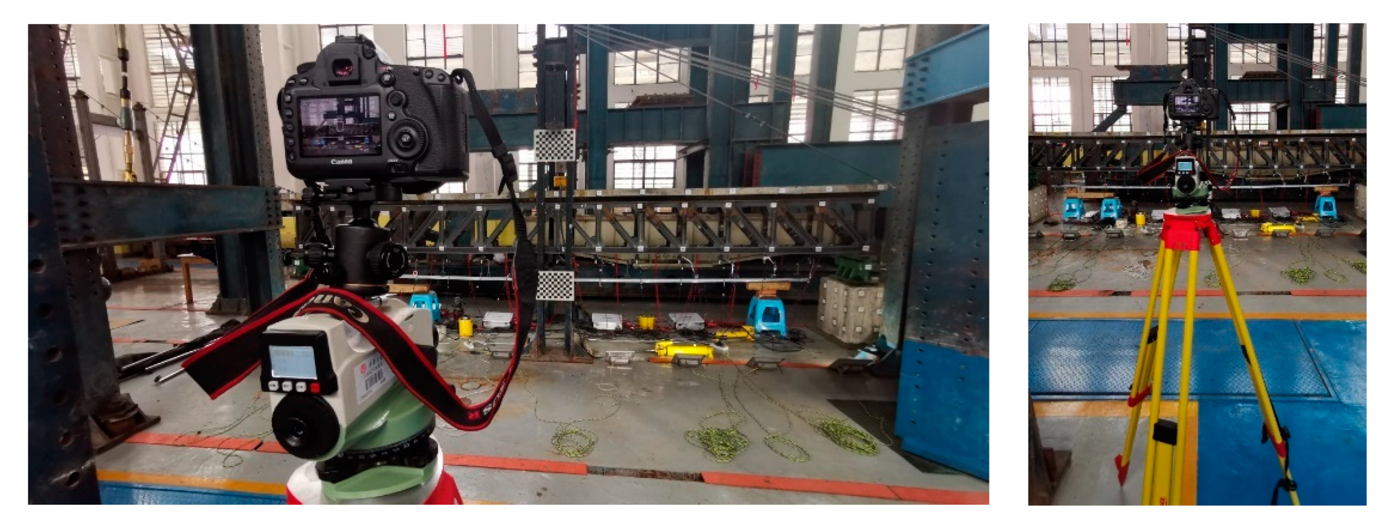
Figure 7.
Arrangement of the dial indicators.
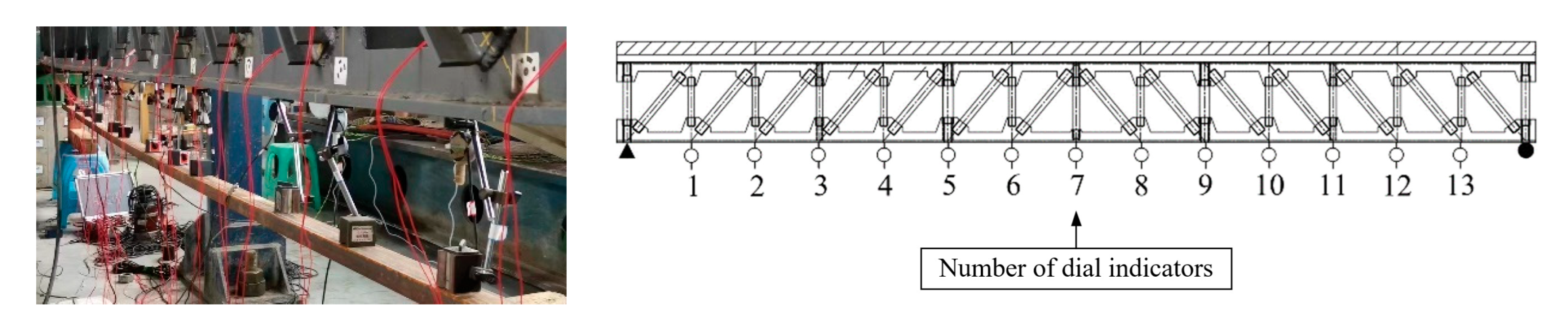
Figure 8.
Three-dimensional laser scanning validation test of the beam. (a) The beam’s code marks. (b) Leica P50 laser scanner scanning the beam.
Figure 8.
Three-dimensional laser scanning validation test of the beam. (a) The beam’s code marks. (b) Leica P50 laser scanner scanning the beam.
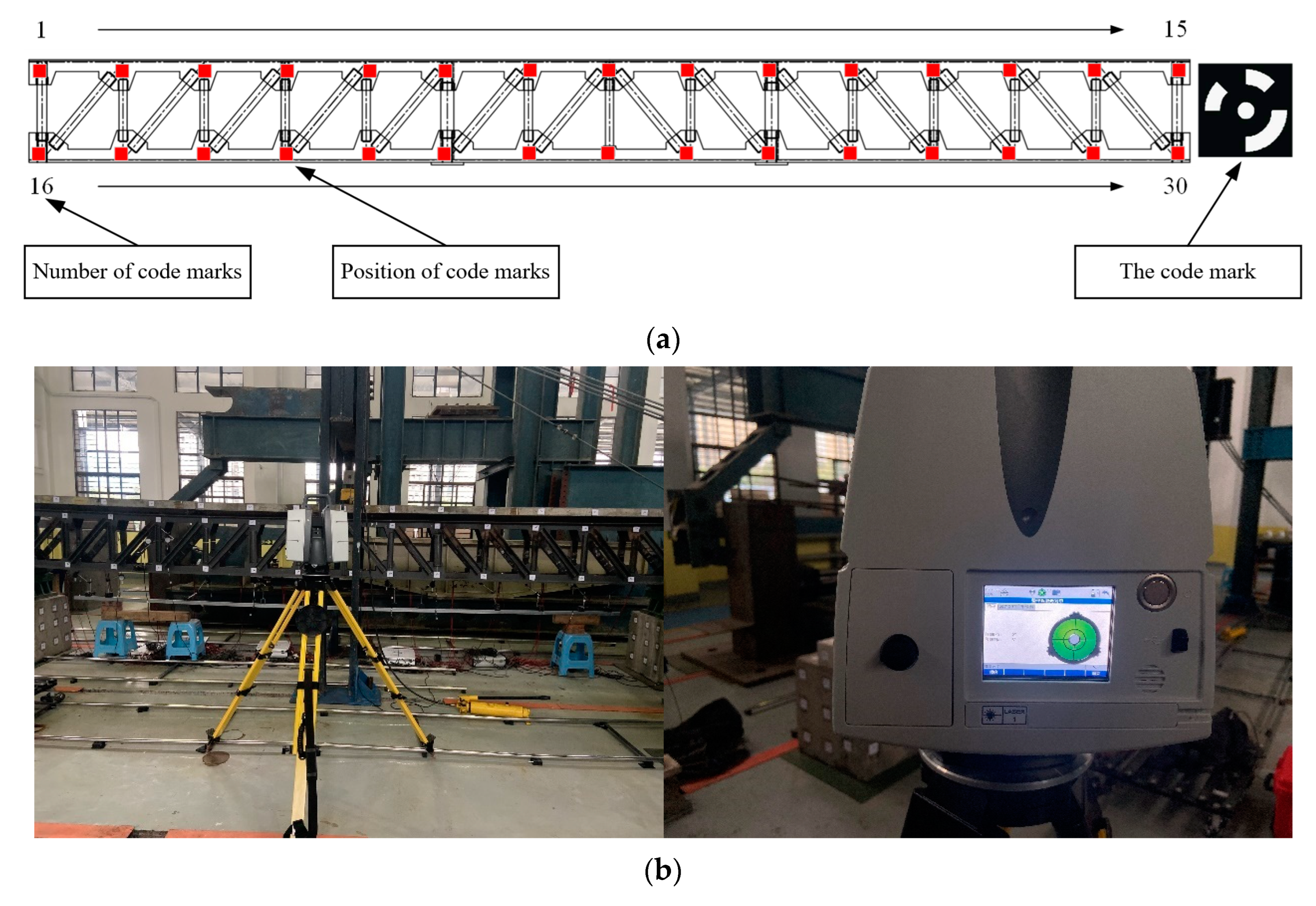
Figure 9.
The mid-span load point of the beam.
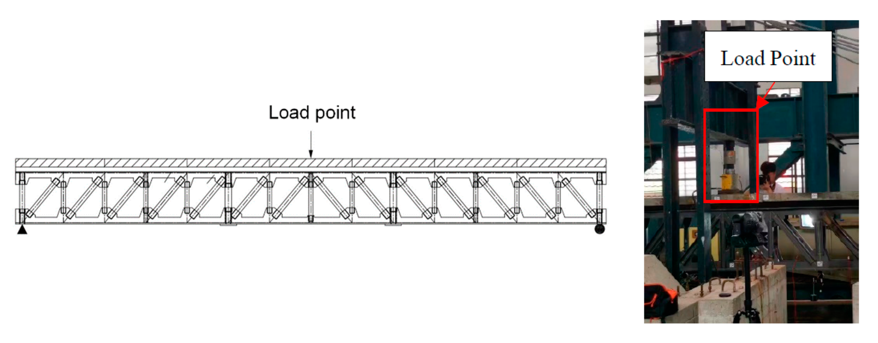
Figure 10.
Calibration line on the vertical member of the beam.
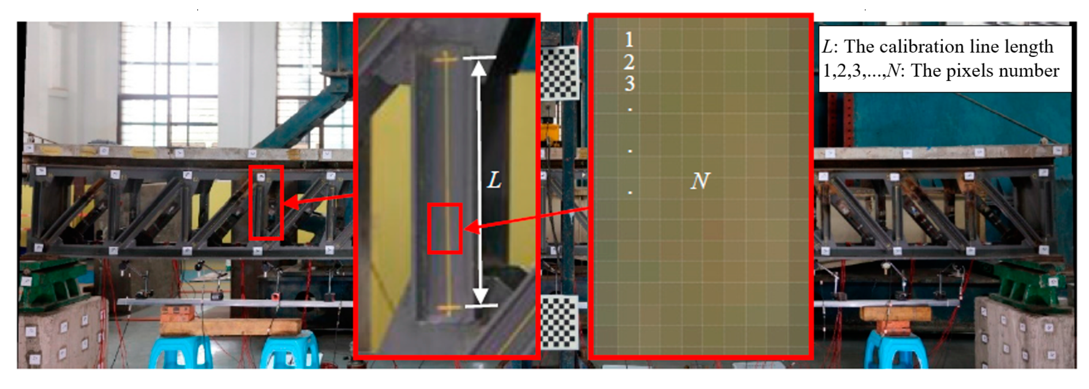
Figure 11.
Original image and feature point image of the beam. (a) Beam’s image. (b) Beam’s feature points.
Figure 11.
Original image and feature point image of the beam. (a) Beam’s image. (b) Beam’s feature points.
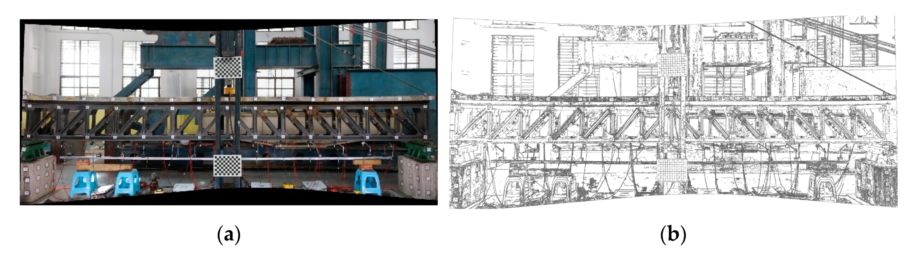
Figure 12.
Calculated position of the beam’s multi-point displacement.
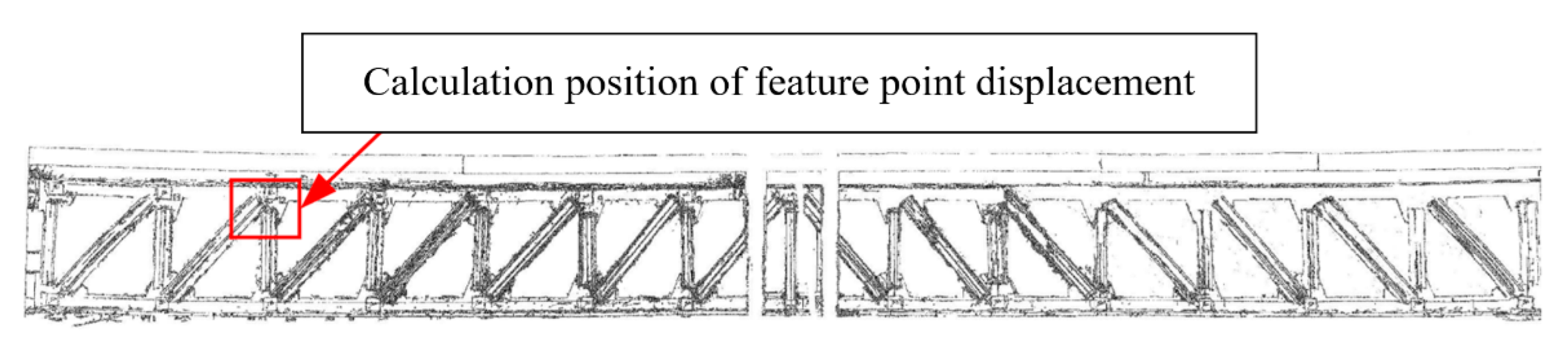
Figure 13.
Multi-point displacement initial calculation results for the beam’s local area. (a) Initial calculation results at 100 kN. (b) Initial calculation results at 200 kN. (c) Initial calculation results at 300 kN. (d) Initial calculation results at 400 kN.
Figure 13.
Multi-point displacement initial calculation results for the beam’s local area. (a) Initial calculation results at 100 kN. (b) Initial calculation results at 200 kN. (c) Initial calculation results at 300 kN. (d) Initial calculation results at 400 kN.
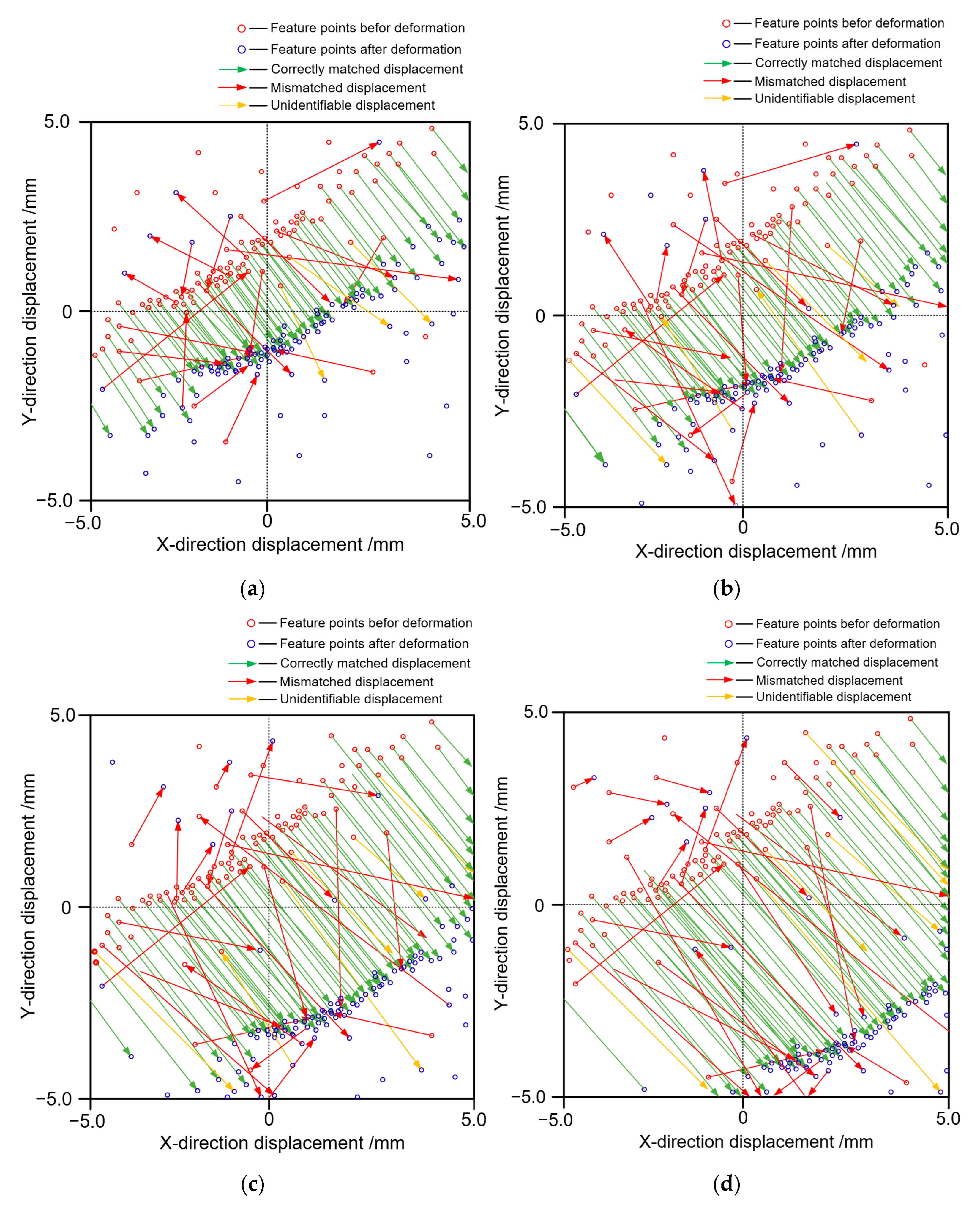
Figure 14.
Beam’s edge line extraction results. (a) Edge position. (b) Edge deformation under load levels 0–400 kN.
Figure 14.
Beam’s edge line extraction results. (a) Edge position. (b) Edge deformation under load levels 0–400 kN.
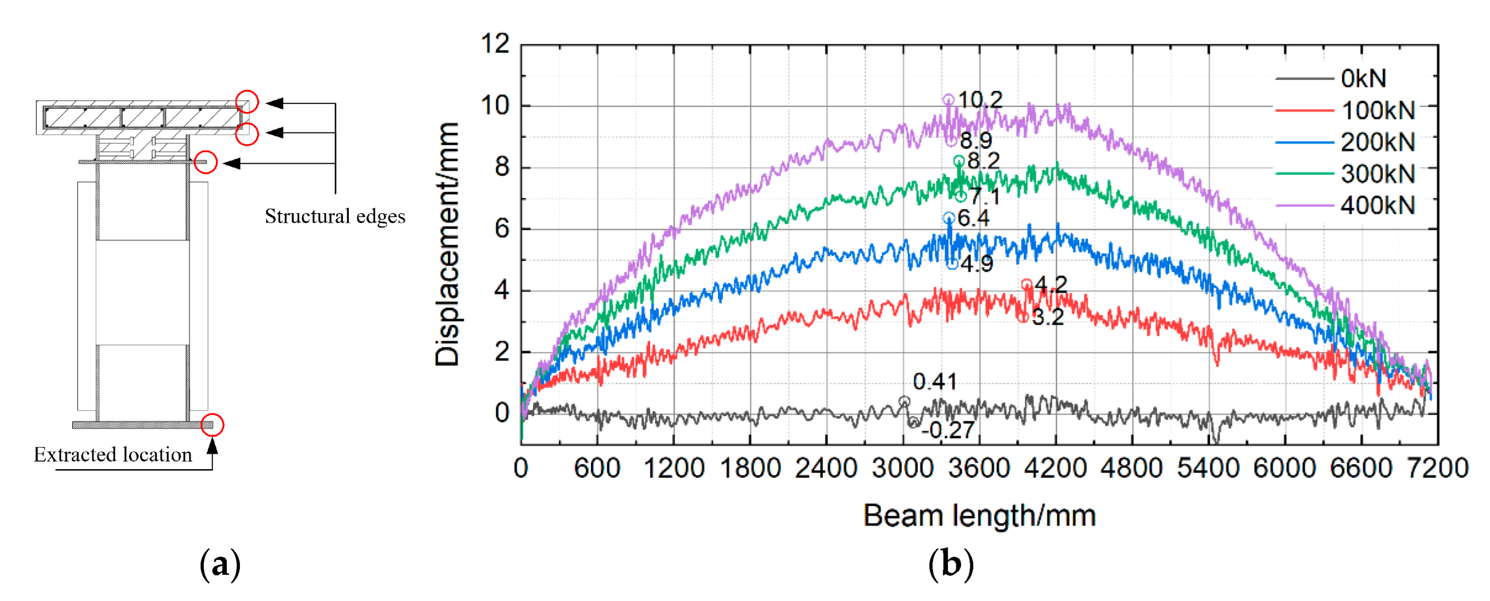
Figure 15.
Beam’s edge deflection curve. (a) Similarity of the edge distribution. (b) The beam’s deflection curve.
Figure 15.
Beam’s edge deflection curve. (a) Similarity of the edge distribution. (b) The beam’s deflection curve.
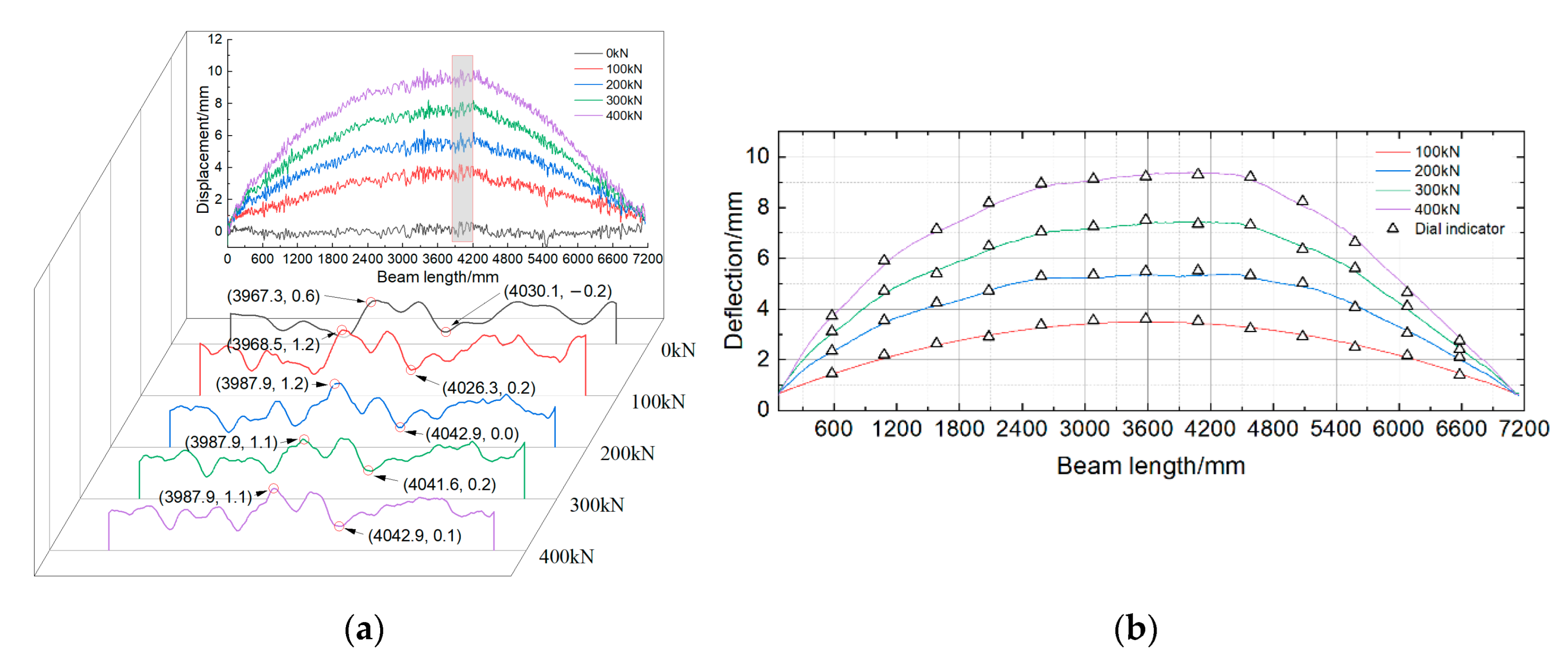
Figure 16.
Test beam’s edge rotation angle calculation results under various load levels. (a) Test beam’s edge rotation angle (100 kN). (b) Test beam’s edge rotation angle (200 kN). (c) Test beam’s edge rotation angle (300 kN). (d) Test beam’s edge rotation angle (400 kN).
Figure 16.
Test beam’s edge rotation angle calculation results under various load levels. (a) Test beam’s edge rotation angle (100 kN). (b) Test beam’s edge rotation angle (200 kN). (c) Test beam’s edge rotation angle (300 kN). (d) Test beam’s edge rotation angle (400 kN).
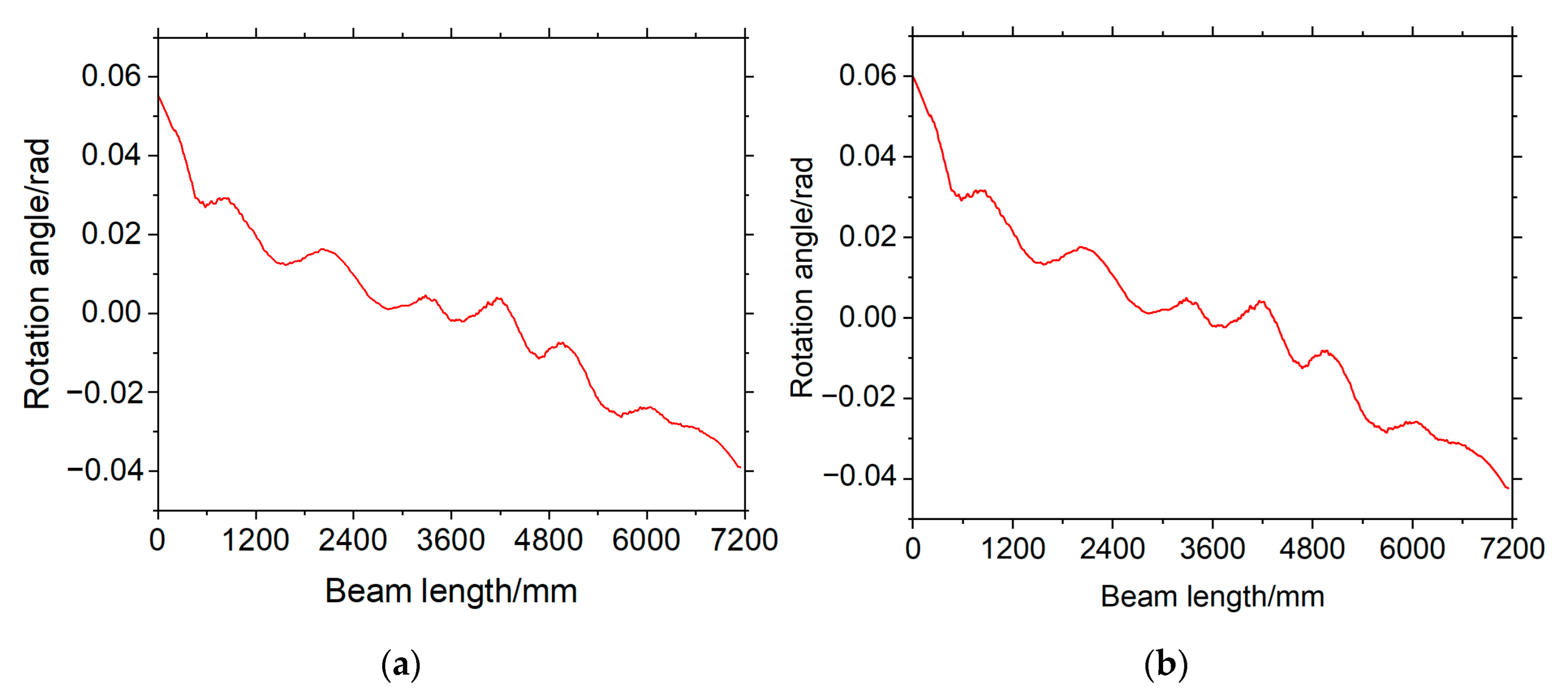
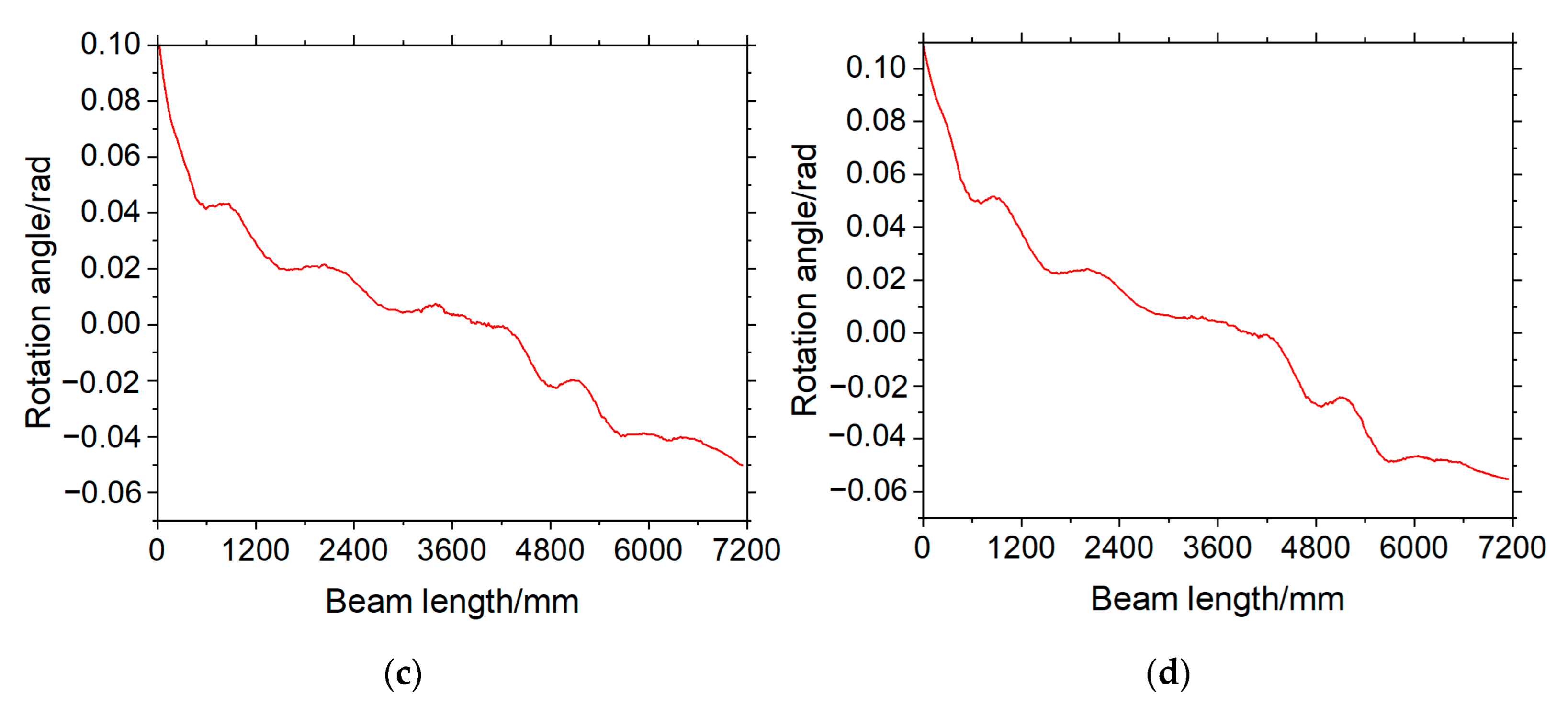
Figure 17.
Displacement mismatch elimination method.
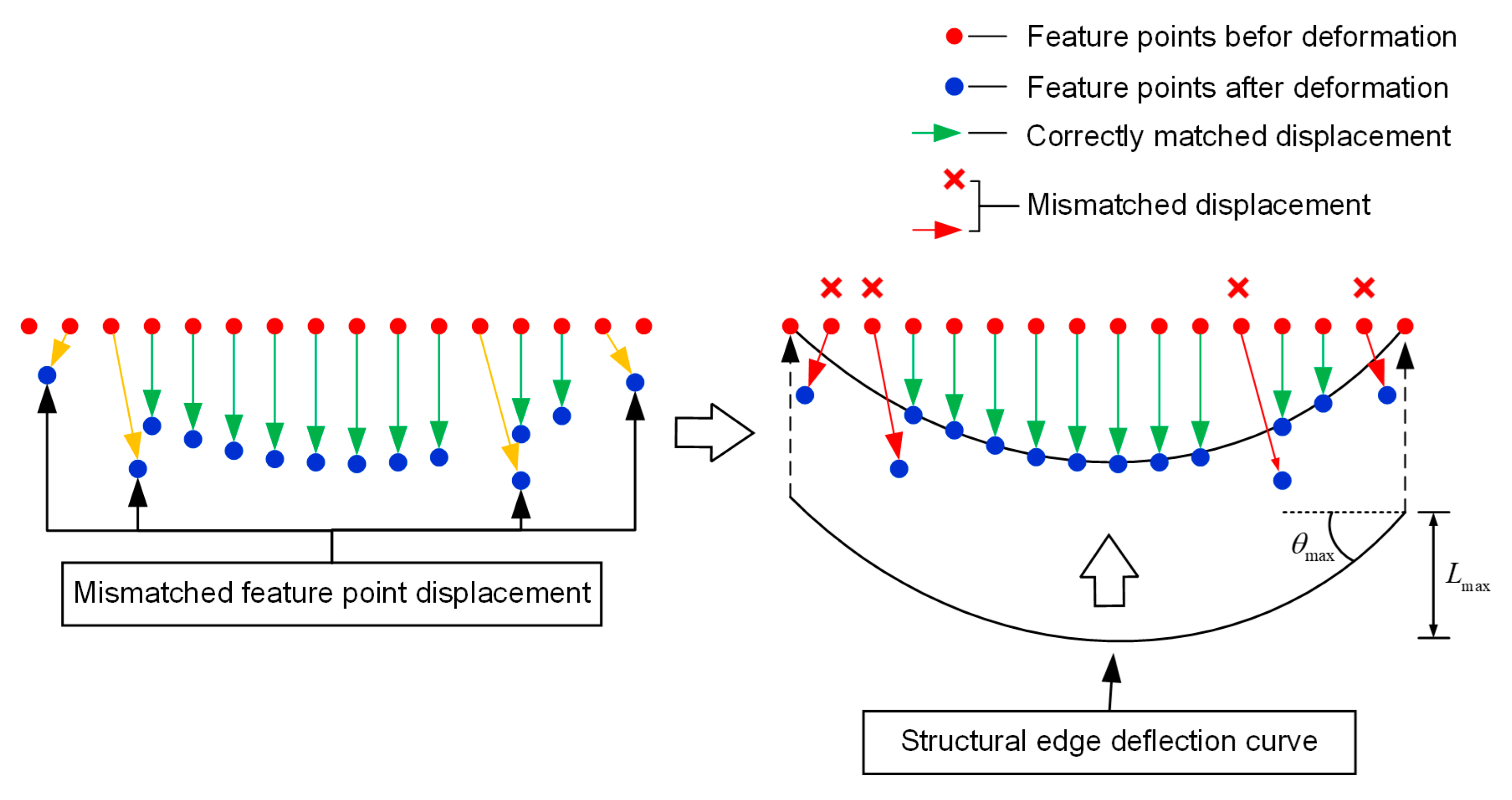
Figure 18.
Rotation angle threshold mismatch elimination process.
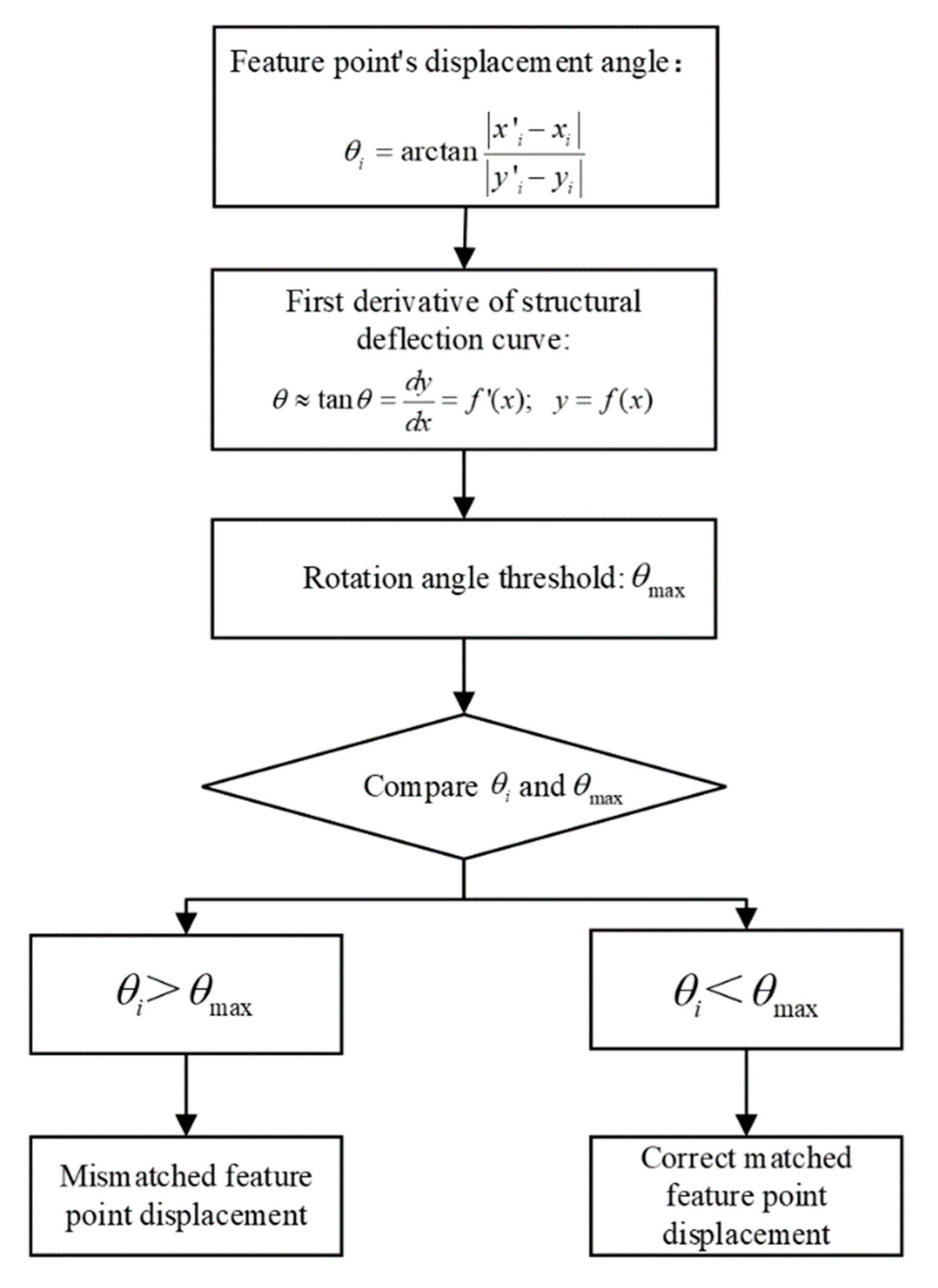
Figure 19.
Results for the multi-point displacement mismatch elimination. (a) After mismatch elimination (100 kN). (b) After mismatch elimination (200 kN). (c) After mismatch elimination (300 kN). (d) After mismatch elimination (400 kN).
Figure 19.
Results for the multi-point displacement mismatch elimination. (a) After mismatch elimination (100 kN). (b) After mismatch elimination (200 kN). (c) After mismatch elimination (300 kN). (d) After mismatch elimination (400 kN).
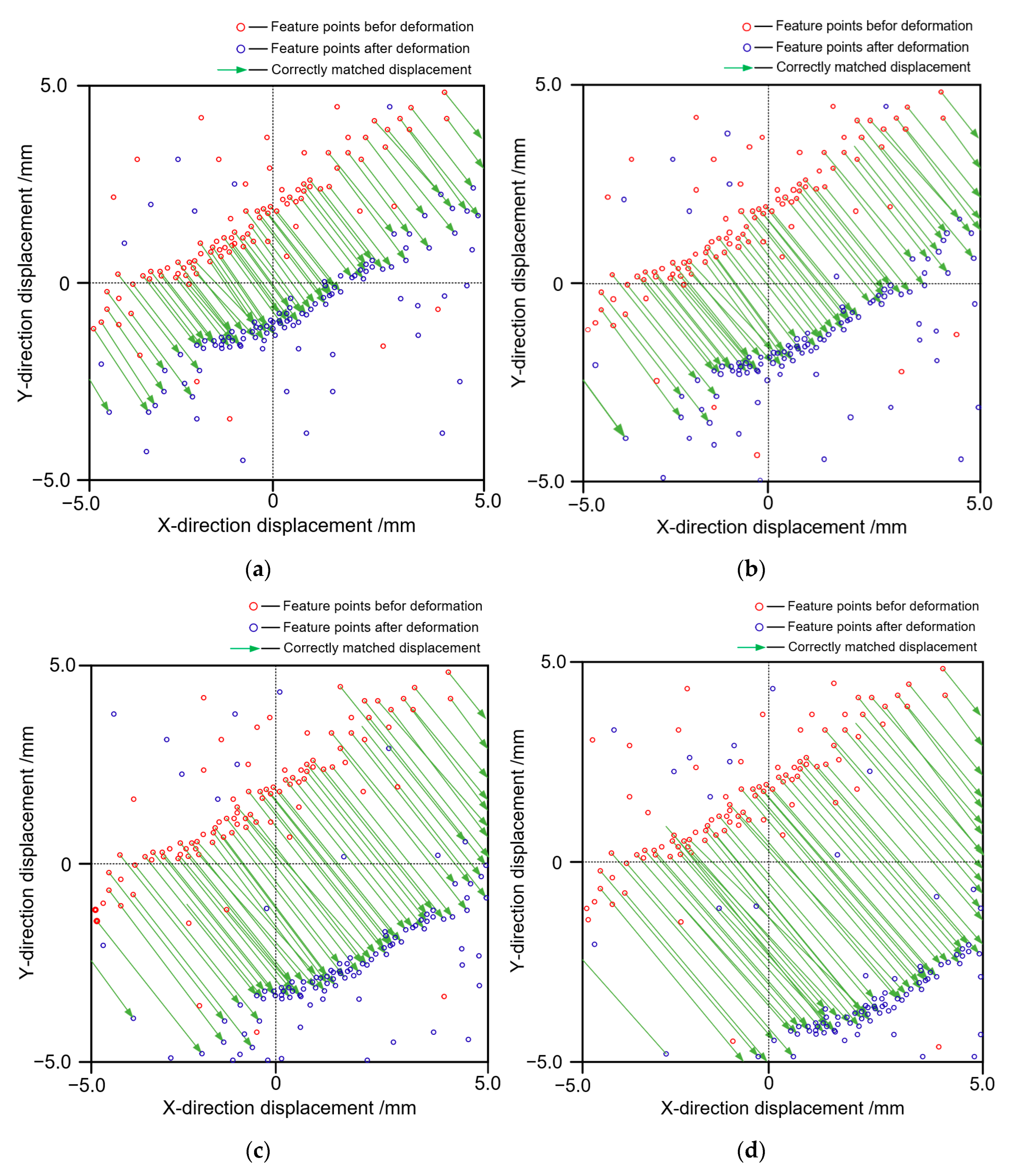
Figure 20.
Beam’s multi-point displacement calculation results under various load levels. (a) Beam’s multi-point displacement (100 kN). (b) Beam’s multi-point displacement (200 kN). (c) Beam’s multi-point displacement (300 kN). (d) Beam’s multi-point displacement (400 kN).
Figure 20.
Beam’s multi-point displacement calculation results under various load levels. (a) Beam’s multi-point displacement (100 kN). (b) Beam’s multi-point displacement (200 kN). (c) Beam’s multi-point displacement (300 kN). (d) Beam’s multi-point displacement (400 kN).
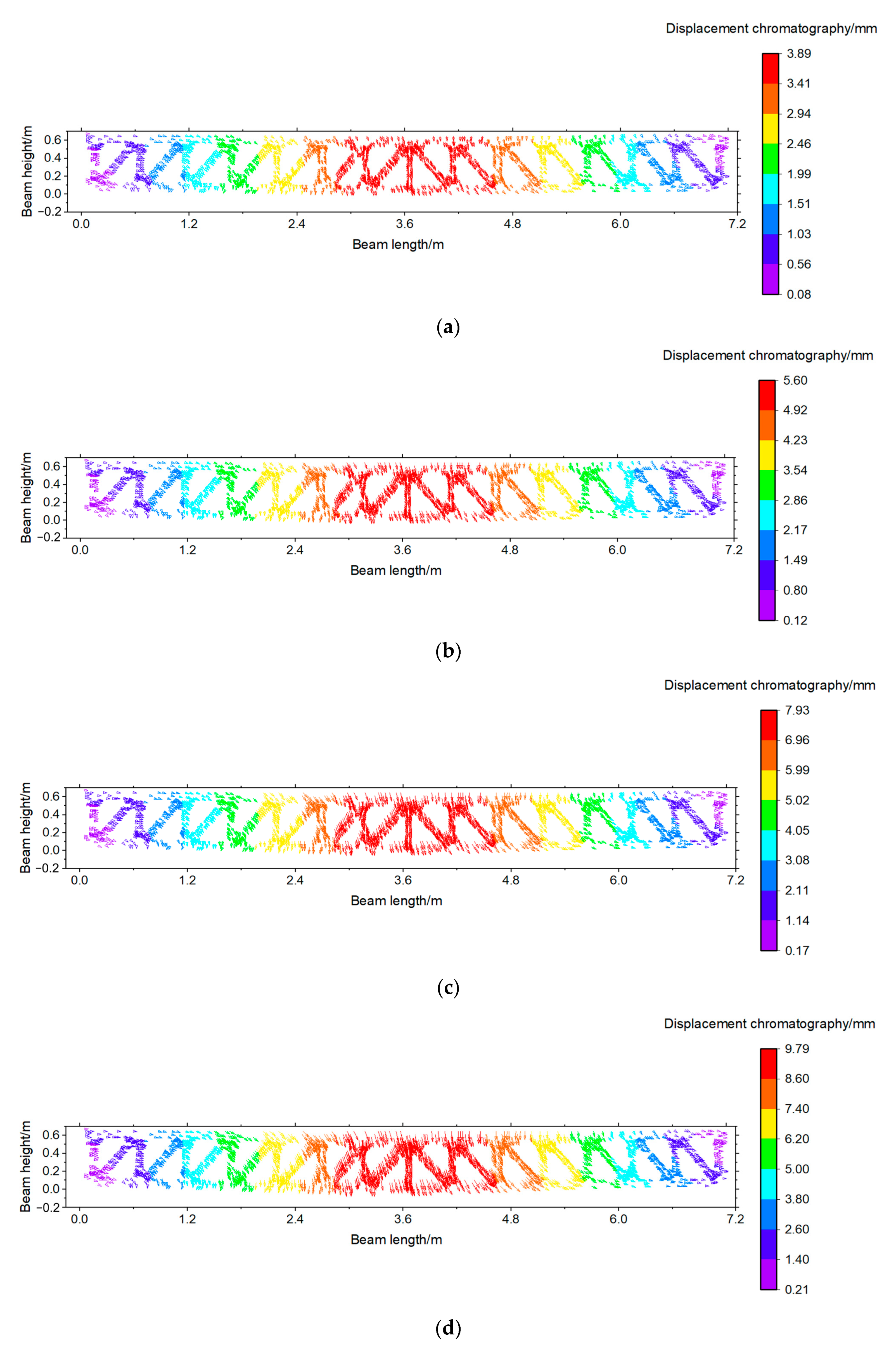
Figure 21.
Three-dimensional laser-scanned model of the beam.
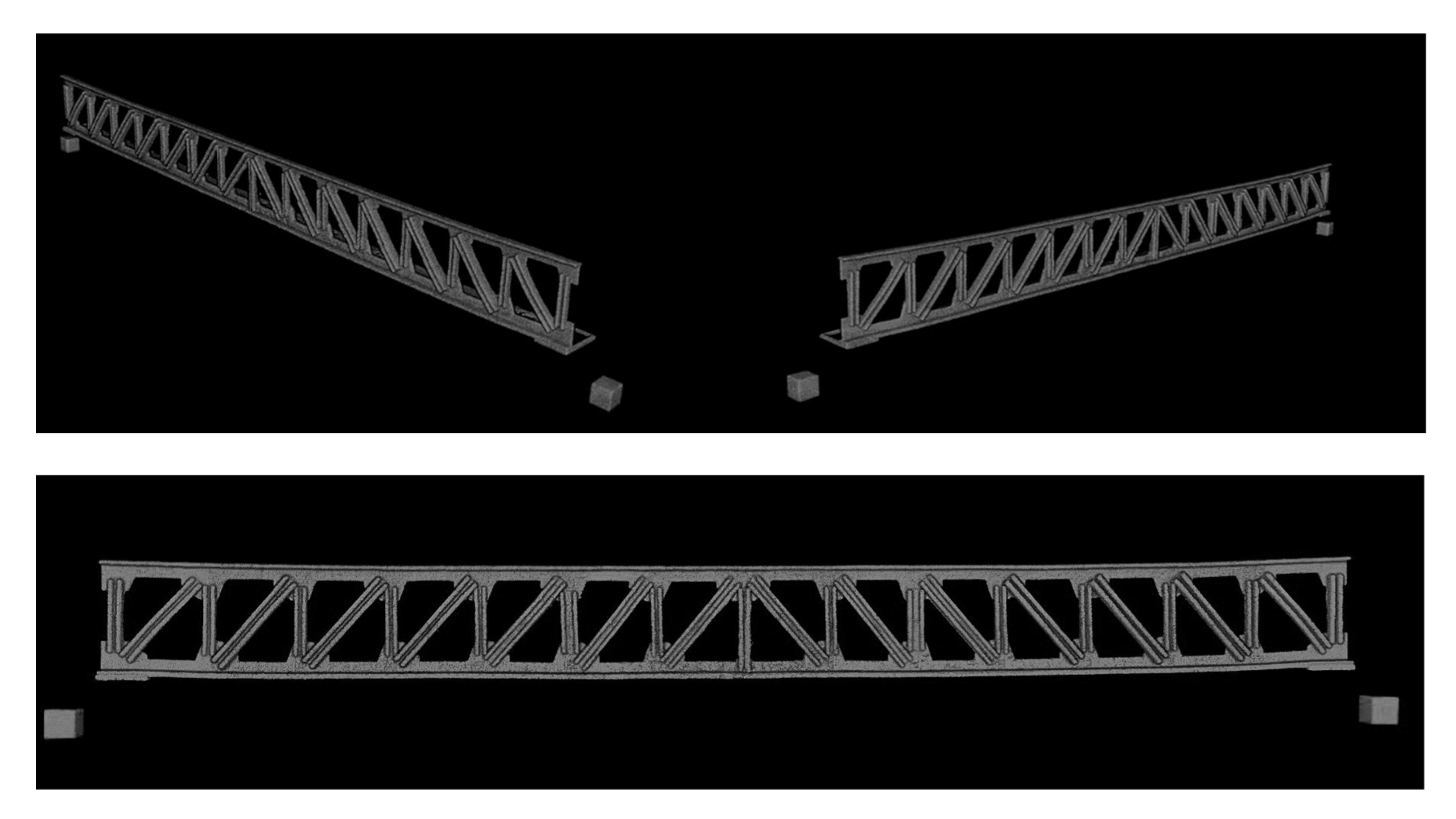
Figure 22.
Deformation chromatograms of the beam under various load conditions. (a) Beam’s deformation chromatography (100 kN). (b) Beam’s deformation chromatography (200 kN). (c) Beam’s deformation chromatography (300 kN). (d) Beam’s deformation chromatography (400 kN).
Figure 22.
Deformation chromatograms of the beam under various load conditions. (a) Beam’s deformation chromatography (100 kN). (b) Beam’s deformation chromatography (200 kN). (c) Beam’s deformation chromatography (300 kN). (d) Beam’s deformation chromatography (400 kN).


Table 1.
Monitoring camera’s parameters.
| Pixels | Sensor | Data Interface | Image Frame |
|---|---|---|---|
| 102 million | 43.8 × 32.9 mm | USB 3.0 | 11,648 × 8736 |
| Pixel size | Lens model | Relative aperture of lens | Focal length |
| 3.76 μm | GF 32–64/4 R LM WR | F4.0–F32 | 32–64 mm |
Table 2.
The test’s monitoring resolution.
| Member Nos. | N | L (mm) | Calibration Results L/N (mm/pixel) | Average |
|---|---|---|---|---|
| 1–16 | 1975 | 386.24 | 0.20 | 0.18 mm/pixel |
| 2–17 | 1978 | 349.25 | 0.18 | |
| 3–18 | 1987 | 327.83 | 0.16 | |
| 4–19 | 1980 | 332.91 | 0.17 | |
| 5–20 | 1968 | 366.79 | 0.19 | |
| 6–21 | 1989 | 327.91 | 0.16 | |
| 7–22 | 1980 | 359.12 | 0.18 | |
| 8–23 | 1992 | 345.13 | 0.17 | |
| 9–24 | 1989 | 312.15 | 0.16 | |
| 10–25 | 1992 | 387.54 | 0.19 | |
| 11–26 | 1991 | 381.28 | 0.19 | |
| 12–27 | 1983 | 331.53 | 0.17 | |
| 13–28 | 1982 | 349.27 | 0.18 | |
| 14–29 | 1981 | 339.25 | 0.17 | |
| 15–30 | 1989 | 351.72 | 0.18 |
Table 3.
Validation of the beam’s edge deflection.
| Load | Dial Indicator No. | Dial Indicator Value (mm) | Calculated Value (mm) | Error (%) |
|---|---|---|---|---|
| 100 kN | 1 | 1.45 | 1.42 | 2.07% |
| 2 | 2.19 | 2.17 | 0.91% | |
| 3 | 2.63 | 2.57 | 2.28% | |
| 4 | 2.90 | 2.97 | 2.41% | |
| 5 | 3.37 | 3.26 | 3.26% | |
| 6 | 3.55 | 3.42 | 3.66% | |
| 7 | 3.61 | 3.49 | 3.32% | |
| 8 | 3.53 | 3.44 | 2.55% | |
| 9 | 3.22 | 3.27 | 1.55% | |
| 10 | 2.91 | 2.99 | 2.75% | |
| 11 | 2.53 | 2.59 | 2.37% | |
| 12 | 2.16 | 2.08 | 3.70% | |
| 13 | 1.40 | 1.45 | 3.57% | |
| 200 kN | 1 | 2.34 | 2.32 | 0.85% |
| 2 | 3.55 | 3.63 | 2.25% | |
| 3 | 4.24 | 4.12 | 2.83% | |
| 4 | 4.73 | 4.72 | 0.21% | |
| 5 | 5.29 | 5.19 | 1.89% | |
| 6 | 5.34 | 5.24 | 1.87% | |
| 7 | 5.49 | 5.34 | 2.73% | |
| 8 | 5.51 | 5.32 | 3.45% | |
| 9 | 5.33 | 5.26 | 1.31% | |
| 10 | 5.03 | 4.88 | 2.98% | |
| 11 | 4.07 | 4.16 | 2.21% | |
| 12 | 3.04 | 3.13 | 2.96% | |
| 13 | 2.11 | 2.01 | 4.74% | |
| 300 kN | 1 | 3.11 | 3.03 | 2.57% |
| 2 | 4.72 | 4.85 | 2.75% | |
| 3 | 5.41 | 5.53 | 2.22% | |
| 4 | 6.48 | 6.34 | 2.16% | |
| 5 | 7.05 | 6.99 | 0.85% | |
| 6 | 7.16 | 7.17 | 0.14% | |
| 7 | 7.32 | 7.39 | 0.96% | |
| 8 | 7.36 | 7.42 | 0.82% | |
| 9 | 7.31 | 7.25 | 0.82% | |
| 10 | 6.37 | 6.46 | 1.41% | |
| 11 | 5.61 | 5.49 | 2.14% | |
| 12 | 4.11 | 4.00 | 2.68% | |
| 13 | 2.41 | 2.46 | 2.07% | |
| 400 kN | 1 | 3.73 | 3.71 | 0.54% |
| 2 | 5.88 | 6.11 | 3.91% | |
| 3 | 7.16 | 7.06 | 1.40% | |
| 4 | 8.19 | 8.03 | 1.95% | |
| 5 | 8.96 | 8.78 | 2.01% | |
| 6 | 9.13 | 9.09 | 0.44% | |
| 7 | 9.47 | 9.32 | 1.58% | |
| 8 | 9.22 | 9.37 | 1.63% | |
| 9 | 8.94 | 9.13 | 2.13% | |
| 10 | 8.35 | 8.07 | 3.35% | |
| 11 | 6.64 | 6.79 | 2.26% | |
| 12 | 4.65 | 4.74 | 1.94% | |
| 13 | 2.76 | 2.86 | 3.62% |
Table 4.
Rotation angle thresholds.
| Load Level | Rotation Angle Threshold (Rad) |
|---|---|
| 100 kN | 0.055 |
| 200 kN | 0.059 |
| 300 kN | 0.098 |
| 400 kN | 0.110 |
Table 5.
Validation of multi-point displacement synchronous monitoring results.
| Load | Code Mark No. | Validation Value (mm) | Calculated Value (mm) | Error (%) |
|---|---|---|---|---|
| 400 kN | 1 | 1.00 | 1.03 | 3.26% |
| 2 | 4.96 | 4.75 | 4.29% | |
| 3 | 7.82 | 8.29 | 5.95% | |
| 4 | 9.52 | 9.84 | 3.35% | |
| 5 | 10.89 | 11.23 | 3.05% | |
| 6 | 11.92 | 11.13 | 6.60% | |
| 7 | 12.14 | 12.32 | 1.42% | |
| 8 | 12.60 | 13.11 | 4.12% | |
| 9 | 12.26 | 12.57 | 2.49% | |
| 10 | 11.89 | 12.22 | 2.80% | |
| 11 | 11.11 | 11.38 | 2.51% | |
| 12 | 8.83 | 9.28 | 5.12% | |
| 13 | 6.18 | 6.52 | 5.38% | |
| 14 | 3.67 | 3.99 | 8.70% | |
| 15 | 0.92 | 0.95 | 3.52% | |
| 16 | 0.96 | 0.91 | 4.97% | |
| 17 | 5.00 | 4.68 | 6.38% | |
| 18 | 7.95 | 8.26 | 3.85% | |
| 19 | 9.32 | 9.74 | 4.42% | |
| 20 | 10.96 | 11.19 | 2.06% | |
| 21 | 11.90 | 11.60 | 2.57% | |
| 22 | 12.29 | 12.78 | 4.00% | |
| 23 | 12.40 | 12.85 | 3.65% | |
| 24 | 12.53 | 12.15 | 2.99% | |
| 25 | 12.50 | 12.07 | 3.48% | |
| 26 | 11.12 | 11.65 | 4.81% | |
| 27 | 8.31 | 8.82 | 6.08% | |
| 28 | 6.00 | 5.50 | 8.31% | |
| 29 | 3.82 | 3.92 | 2.70% | |
| 30 | 0.81 | 0.84 | 3.54% |
Disclaimer/Publisher’s Note: The statements, opinions and data contained in all publications are solely those of the individual author(s) and contributor(s) and not of MDPI and/or the editor(s). MDPI and/or the editor(s) disclaim responsibility for any injury to people or property resulting from any ideas, methods, instructions or products referred to in the content. |
© 2023 by the authors. Licensee MDPI, Basel, Switzerland. This article is an open access article distributed under the terms and conditions of the Creative Commons Attribution (CC BY) license (https://creativecommons.org/licenses/by/4.0/).
Share and Cite
MDPI and ACS Style
Chu, X.; Zhou, Z.; Zhu, W.; Duan, X. Multi-Point Displacement Synchronous Monitoring Method for Bridges Based on Computer Vision. Appl. Sci. 2023, 13, 6544. https://doi.org/10.3390/app13116544
AMA Style
Chu X, Zhou Z, Zhu W, Duan X. Multi-Point Displacement Synchronous Monitoring Method for Bridges Based on Computer Vision. Applied Sciences. 2023; 13(11):6544. https://doi.org/10.3390/app13116544
Chicago/Turabian StyleChu, Xi, Zhixiang Zhou, Weizhu Zhu, and Xin Duan. 2023. "Multi-Point Displacement Synchronous Monitoring Method for Bridges Based on Computer Vision" Applied Sciences 13, no. 11: 6544. https://doi.org/10.3390/app13116544
Note that from the first issue of 2016, this journal uses article numbers instead of page numbers. See further details here.