
Building Energy Flexibility Assessment in Mediterranean Climatic Conditions: The Case of a Greek Office Building

Process Equipment Design Laboratory, Department of Mechanical Engineering, Aristotle University of Thessaloniki, 54124 Thessaloniki, Greece
*
Author to whom correspondence should be addressed.
Appl. Sci. 2023, 13(12), 7246; https://doi.org/10.3390/app13127246
Submission received: 1 May 2023
/
Revised: 10 June 2023
/
Accepted: 15 June 2023
/
Published: 17 June 2023
(This article belongs to the Special Issue Sustainability in Energy and Buildings: Future Perspectives and Challenges)
Abstract
:The EU energy and climate policy has set quantitative goals for decarbonization based on the energy efficiency and the evolution of energy systems. The utilization of demand side flexibility can help towards this direction and achieve the target of higher levels of penetration in regard to intermittent renewable energy production and carbon emission reduction. This paper presents a simulation-based assessment of thermal flexibility in a typical office building in Greece, which is a representative Mediterranean country. The use of variable speed heat pumps coupled with hydronic terminal units was evaluated. The research focused mainly on the evaluation of energy flexibility offered by energy stored in the form of thermal energy by utilizing the building’s thermal mass. The demand response potential under hourly CO2eq intensity and energy prices was investigated. The flexibility potential was evaluated under different demand response strategies, and the effect of demand response on energy consumption, operational costs, CO2eq emissions and thermal comfort was analyzed and discussed. The results showed that both control strategies based on both the CO2eqintensity signal and spot price signal have, in some cases, the potential for cost and emission savings, and in other cases, the potential to depreciate in terms of emissions and cost the increase of energy consumption due to load shifting.
1. Introduction
In recent decades, consumer demand for greater living standards has increased along with global electricity use [1]. This rise in global energy consumption, forecasted declines in fossil fuel supply and signs of escalating consequences of global warming have all contributed to an increased focus in RES research. Because of the intrinsic unpredictability that characterizes RES, instability risk in the energy network grows as RES become more prevalent in covering demand [2]. The necessity to control demand and guarantee flexible energy usage is reinforced by the requirement for network stability. Buildings are anticipated to be a key player in this change by supplying the power grid with their energy flexibility to help meet the demands of energy networks [2]. To this end, and in line with the updated European regulations requiring a low-carbon built environment [3], it is imperative that buildings are designed with energy efficiency and decarbonization in mind. To this end, flexible operation and smart energy use in buildings are seen as key strategies for mitigating greenhouse gas emissions and ensuring resilient energy system operations [4].
Buildings can offer their energy flexibility in multiple ways. One of the main methods for offering flexibility is thermal energy storage. The thermal mass of a building can be used for load shifting when an energy deficit is detected since it can store thermal energy for short periods of time [5].
Office buildings are seen as the best option for implementing DR programs due to their high energy usage and generally superior automation infrastructure compared to residential buildings [6]. Commercial HVAC, lighting and other electrical equipment in office buildings can adjust their operational profile to support the energy grid.
Several researchers have come to appreciate the importance of buildings as a source of energy flexibility to the energy grid and tried to quantify the demand side flexibility of the building sector by implementing DR in buildings and their energy systems. In their research [7], they tried to quantify the flexibility that a building with CHP and energy storage can offer, by considering the magnitude of a CHP operation’s delay or forced operation time. Arteconi et al., 2019 [8] introduced a multicriteria indicator and tried to quantify the energy flexibility of a residential building with AWHP and TES. De Coninck and Helsen in 2016 [9] introduced cost curves as a metric for measuring flexibility that is applicable to a wide variety of building typologies and energy systems. In [10], power shifting indexes were employed to evaluate an office building’s flexibility under model predictive control. Masy et al., 2015 [11], developed a generic flexibility assessment methodology that was applied to various building typologies equipped with heat pumps. In [12,13], indicators that cover time, size and cost were used to quantify the energy storage in building thermal mass as a mean of flexibility in different building typologies. D’Ettorre et al., 2019 [14], implemented different DR scenarios to assess the flexibility of a building equipped with a hybrid heating system with thermal energy storage located in Italy. Several temperature regulation strategies were implemented in detailed resistance–capacitance models of various buildings in order to quantify their demand response potential in [15].
Several researches studied the impact of DR control on equivalent carbon dioxide emissions. The authors of [16,17,18] tested the implementation of MPC in residential buildings. Ιn every case, a reduction in dioxide emissions was observed. Other researchers studied the implementation of two different CO2 MPCs to a large commercial building with two different HVAC settings and found decreases in emissions, especially in the case of exploiting renewable energy [19]. Vigna et al., 2021 [20], assessed building clusters with different thermal mass characteristics, which consisted of residential buildings with ideal heating systems, under CO2 forcing factor smart control. Only two papers were found in the literature that test the implementation of RBC, either by considering CO2 forcing factors [21] or just studying the impact of economic RBC on carbon emissions [22].
The purpose of this research was to evaluate the energy flexibility of an office building in the Mediterranean area. The study used electricity market data and examined two types of PRBCs: economic PRBC and environmental PRBC. To achieve this goal, classic energy, and environmental and economic indicators were used, as well as energy flexibility indicators. The key innovations of this paper are the initial assessment of energy flexibility in terms of environmental performance, which is quite limited in the literature, especially for office buildings. In addition, PRBC controls were implemented with the aim of reducing energy costs and the carbon footprint using data from the energy market. Another contribution is the detailed modelling and simulation of both the building and its heating system. In most cases when a detailed building is simulated, the HVAC systems are simplified, and in cases when a detailed model of HVAC system is realized, a simplified building model is used, like a resistance–capacitance model. Finally, a holistic analysis was conducted, and the flexibility was evaluated with multiple indicators to produce more detailed results.
The remainder of the paper is structured as follows: The weather and electricity market data, the building, the operating conditions, the installed HVAC systems, and the modelling and simulation methodology, are all described in Section 2. Section 3 includes the description of the implemented control algorithms. Section 4 describes the performance indicators. The findings under the various demand response strategies are presented and discussed in Section 5, before the paper is concluded in Section 6.
2. Methodology
With the target of a building energy flexibility evaluation, a building and its heating system were modeled. As part of the study, an office building in the area of Thessaloniki was selected. Most studies investigate the energy flexibility that residential buildings can offer. This building is building D of the polytechnic school of AUTH. It is a building that is characterized by various uses of spaces with it predominantly being used as an office. The building in its current state meets its heating needs using gas-fired boilers. For the purposes of the study, heating was electrified and the gas-fired boilers were replaced by heat pumps.
2.1. Weather Data
Thessaloniki’s mild, warm, subtropical Mediterranean climate (Koppen–Geiger classification: Csa) results in relatively low heating and cooling requirements. Because of the data availability regarding the electricity market, the simulations were conducted using 2022 weather data. The weather for 2022 was not typical weather for Thessaloniki, as it was relatively hot throughout the year with less heating degree days compared to previous years.
In Figure 1, we notice that the average monthly temperature was high throughout the year, with a minimum average monthly temperature of 6 degrees in January. The average monthly global horizontal irradiance remained above 80 W/m2 throughout the year reaching the maximum value of about 330 W/m2 in July (Figure 2). High levels of relative humidity were present compared to average Greece levels, with a minimum value of about 12%, a maximum value reaching around 100%, and average around 50%.
2.2. Electricity Market Data
For the implementation of the control methods for the heating system, historical data of the Greek energy market were used [23]. The price data refer to hourly wholesale market prices for the whole year. We noticed in Figure 3 that prices varied between approximately 50 EUR/MWh and 900 EUR/MWh. The lowest prices were observed during the winter months and especially in the months of October, January and February, while the highest prices were observed during the summer period and especially in the month of August, due to the particularly increased demand because of tourism. It was also evident that the lowest prices occurred during nighttime (24:00–6:00), while the price seemed to be maximized during the early morning hours (7:00–10:00) and during the afternoon hours (18:00–22:00). On the contrary, in terms of dioxide emissions [24], the participation of RES and especially PV was evident since the minimum daily values were observed during the hours of sunshine (9:00–17:00) and the minimum values on an annual basis were observed during the transitional periods (autumn and spring), both due to the increased production of PV energy compared to the winter season and due to the reduced demand compared to the summer season (Figure 4). In this case, the values ranged between 100 and 550 gCO2/kWh.
2.3. Building and Thermal Zoning
Building D’ of the Aristotle University of Thessaloniki’s Faculty of Engineering, which is located between Egnatia and 3rd September streets, is the building under the investigation in this study. Building D’, which has ten floors (including the ground floor), houses the secretariats of the various departments as well as the offices of the faculty’s teaching and research staff. Some laboratories are also housed in the basement of the building.
The building’s overall volume and surface area are 44,671,197 m3 and 10,595,451 m2, respectively, of which 29,017,462 m3 and 8,167,691 m2 are heated spaces. The structure has not undergone renovation since it was built, and it is thermally insulated in accordance with the 1979 Greek law on thermal insulation [25]. For the building under consideration, the entire building’s external surface that is exposed to air is A = 8714.90 m2. The window-to-wall ratio is roughly 16%, and the overall area of glazing is 1147.78 m2.
To achieve a more accurate energy analysis, the building under study was divided into 12 thermal zones. Each of the 10 floors comprised a different conditioned thermal zone and the basement and roof were unconditioned thermal zones. On floors 1–9, most of the surface (70%) is occupied by offices, while auxiliary spaces and hallways occupy the remaining area. The zone that corresponds to the ground level of the building is made up of 70% ancillary spaces and 30% offices and secretariats.
2.4. Operating Conditions
There are two different types of uses for this particular building. The main use is as offices, and the second is the use of the hallways and supporting areas. The internal operating conditions of each thermal zone were determined using Technical Chamber of Greece guidelines (T.O.T.E.E. 20701-1), the Greek regulation on buildings’ energy performance (KENAK), and the ASHRAE STANDARD 90.1 [26]. In order to comply with the Energy Performance of Buildings Directive (EPBD), the Greek regulation was recently amended [27]. The selection was made with the objective of offering adequate levels of thermal comfort to all inhabitants [28], and the outcomes are outlined in Table 1. The heating setpoint was taken from the ASHRAE STANDARD, as the Greek regulation’s setpoint of 20 °C was judged insufficient.
2.5. Building Shell and HVAC Systems
2.5.1. Building Shell
The reference building has been thermally insulated in accordance with the Building Regulations for Thermal Insulation [25], as indicated in Section 2.1. Total thermal permeability values for all exposed structural components were determined for both the reference and case A building and are presented in Table 2.
2.5.2. HVAC Systems
Currently, the building is heated by two 90%-efficient natural gas boilers, a high-temperature water distribution system, and a moderately inefficient pipe insulation distribution system. A compensatory mechanism built within the distribution network handles partial loads and boosts the network’s efficiency to 96%. According to the manufacturer’s technical specifications, the total rated power of the boiler systems is 800 kW. Water radiators (AKAN type), complemented with thermostatic controls, make up the terminal heating units, which operate at an efficiency of 89% [28]. In order to be able to implement the DR scenarios and assess the building’s demand response potential, during the modeling process, the existing heating system was replaced with an electric system. The existing system was replaced with a system consisting of a VSHP, a low temperature distribution network and an emission system consisting of hot water radiators.
2.6. Modeling and Simulation
Energy modeling was completed in TRNSYS 18 after the building geometry was modeled using the software environment of SketchUp 2017 [30]. The model was made utilizing details on the dimensions, architectural elements, orientation, and shadings of the real structure (Figure 5 and Figure 6). Every structural parameter, as well as operational parameters, setpoints and schedules, and internal loads, were set up following the import of the building model into TRNSYS. Using the weather files, the essential climatic information (temperature, relative humidity, radiation, etc.) was added to complete the building model. Detailed models of both the building and its heating systems were realized in TRNSYS. The TRNSYS HVAC library only includes single and double speed heat pumps. In order to model the VSHP, the methodology proposed by Toffanin et al., 2019 was used [31].
3. Control Methods
3.1. Reference
The reference scenario set a constant temperature setpoint from 7:00 to 17:00 (working hours) of 21 °C and a setback temperature of 15 °C from 17:00 to 7:00. These setpoints are the most commonly used setpoints for office buildings during the heating period in Greece. During the rest control strategies, the setpoints are increased or decreased by 2 °C so that adequate levels of thermal comfort are maintained. The first DR control scenario is a predefined control strategy and is only used to assess the ability of the building to use its thermal mass for thermal energy storage. The second DR case takes into account power price fluctuations over time and tries to increase electricity consumption for heating during low electricity prices and decrease consumption during high electricity prices, respectively. The third DR scenario works in a similar manner as the second scenario but considers CO2eq intensity instead of electricity prices.
3.2. Predefined Control Strategy
The predefined control scenario was only used to evaluate the ability of the building to store energy in its thermal mass, according to the KPIs proposed by Reynders et al., 2017 [12]. During the implementation of this control strategy, the heating setpoint is increased to 23 °C from 10:00 to 12:00, which is considered a low demand daytime period, considering the selected building typology. The setpoint was kept stable at 21 °C for the rest of the working hours and the setback was maintained at the same levels of the reference scenario. The purpose of this scenario was to calculate the heat stored during the increased setpoint period and assess the efficiency of storage by calculating the thermal losses occurring during the thermal mass activation.
3.3. Cost PRBC
The Cost PRBC uses the working hours spot price data for each day to determine the daily low price and high price limits. The limits arise from the calculation of average price and standard deviation for each day. Then, the setpoints were set to 23 °C during the hours when the price was lower than the average + SD; at 19 °C during the hours when the price is higher than the average + SD; and at 21 °C for the rest of the working hours. The setback is kept stable at 15 °C. This scenario tries to shift energy use away from peak times and toward off-peak times.
3.4. CO2 PRBC
The CO2 PRBC works in a very similar manner with Cost PRBC. The main difference is that instead of energy prices, the CO2eq emissions were used. Again, a high carbon intensity limit and a low carbon intensity limit were calculated for each day. The temperature was kept constant at 23 °C during the times of day when CO2eq emissions are lower than the average + SD; at 19 °C during the hours when the CO2eq emissions is higher than the average + SD; and at 21 °C for the rest of the working hours.
4. Key Performance Indicators (KPIs)
For the evaluation of the different control strategies, various performance indicators were used for the efficient monitoring and control of the systems studied.
- Energy use for heating: The electricity consumption of the heat pump during the heating period.
- Average hourly heat pump power: The electricity used for heating averaged to one hour period.
- Coefficient of performance (COP): This metric reflects the heat pump’s energy efficiency.
- CO2eq emissions: CO2eq intensity is used to measure the level of carbon dioxide equivalent emissions caused by the use of the heating system.
- Cost of energy: The cost that occurs during the operation of the heating system.
- Hours of discomfort: During the operation of the building, some people are not satisfied with the indoor environment thermal conditions. Hours of discomfort are calculated as number of hours that the PMV index value is lower than −0.5 or higher than 1.
- Storage capacity: The heat storage capacity of the thermal mass of a building during a DR event [12].
- Storage efficiency: The portion of energy that may be stored in the structure and utilized later for energy flexibility and thermal comfort provision [12].
- Flexibility: When all of a building’s required heating or cooling energy is utilized at the time of day when energy prices or CO2eq intensity are lowest, the Flexibility index, which assumes values from 0% to 100%, is maximized [11].
5. Results and Discussion
5.1. Demand Response Scenario Implementation
Figure 7 and Figure 8 illustrate the implementation of the control scenarios for 3 consecutive working days. The figures depict from top to bottom the average hourly heat pump power, the indoor air temperature, the PMV index, the COP, the electricity market data and the induced temperature setpoints. The results indicate that the average hourly heat pump power reached around 250 kW for the reference scenario and increases during increased temperature setpoints. The electricity market data indicated a large discrepancy between energy prices and dioxide emissions, since during the hours when the maximum electricity prices were observed, the minimum prices of dioxide emissions appeared and vice versa. This happens because energy production from fossil fuels such as lignite, which are the main source of energy, is characterized by low energy costs but increased emission intensity. Conversely, during the day, due to high demand and production from RES and natural gas base units, prices showed an increase and CO2 emissions decreased significantly. The indoor air temperature and the PMV index values indicate that, during the reference scenario, the heating system cannot efficiently cover the demand with temperatures reaching the setpoint for a few hours each day. On the other hand, during case A, the high internal gains combined with lower heat losses led to cases of slight overheating even for the reference scenario but mostly for the PRBC scenarios when the 23 °C setpoints were forced.
5.2. Evaluation of Thermal Mass Flexibility
In order to evaluate the flexibility that the thermal mass can offer, we used the KPIs proposed by Reynders et al., 2017 [12]. The two main KPIs are storage capacity CADR and storage efficiency ηADR.
The heat storage capacity of the thermal mass of a building during a DR event can be expressed by the available storage capacity (Equation (1)), while taking into account the building’s thermal comfort and varying conditions.
where is the amount of energy consumed during the demand response implementation and is the amount of energy consumed in the same period of time, but under the reference control. The difference between the energy consumption is the amount of energy stored in the thermal mass of the building.
The portion of energy that may be stored in the thermal mass and utilized later for energy flexibility and thermal comfort provision is referred to as the storage efficiency (Equation (2)).
where is the heat storage capacity and is the difference between the energy consumption of the DR scenario and the reference scenario until the building returns to steady state conditions. Essentially, this KPI calculates the amount of stored thermal energy that is possible to be recovered and used.
In their research [12], Reynders et al. calculated those two indicators for a residential building and considering stable ambient conditions of 5 °C and zero solar and internal gains. In our case, we evaluated the average value of the same indicators for several days of the year without considering stable outdoor conditions. Reynders et al. used these indicators as a tool to assess a building’s flexibility during the design stage. We chose to implement the indexes under real operational conditions in order to better capture the operational flexibility of the building.
The results for each building are presented in Table 3. We can observe the lower capacity of the reference scenario and at the same time the lower storage efficiency compared to the case A. The increased capacity of case A is due to the lower heating power needed before the DR setpoints are implemented, which leaves more power reserve when the heat pump tries to reach the 23 °C setpoint. The increased efficiency is mainly attributed to the decreased heat losses of the upgraded building. Compared to the results of [12], we observed a reduced storage efficiency. This is mainly due to the intermittent schedule of the study building, which leads to cycles of charging and discharging of the heat mass of the building, but also due to the residential building shell’s superior thermal properties compared to our building.
5.3. Evaluation of Flexibility in Terms of Cost
The flexibility KPI, proposed by Masy et al., 2015, is used to assess flexibility in terms of cost [11]. The Flexibility index (Equation (3)), which ranges from 0% to 100%, is maximized when all the energy needed is consumed at a time of day when the energy prices are at the lowest levels.
Figure 9 depicts the results for each building (reference, case A) and each control scenario. We noticed that the reference control scenario presents a cost flexibility of about 47%, both for the reference and the case A building. The flexibility increased in the CO2 PRBC scenario to about 48% for both building scenarios. As expected, the Cost PRBC led to the highest cost flexibility index, with values around 51%, with the case A building producing a little higher index value. The small increase between scenarios shows the difficulty in shifting high amounts of energy from high prices periods to low price periods and, at the same time, maintaining adequate thermal comfort levels. Still, even this small increase of about 4% during the Cost PRBC implementation shows that this method works as expected and has the potential of increased cost-efficient operation of heating under DR.
In their research, Masy et al. evaluated the flexibility in terms of cost of a residential building with a heat pump for heating, and various levels of building envelope insulation and heat emission systems [11]. The results showed a flexibility index of approximately 78% for the case of hot-water radiators. We noted that the differences with respect to our results are significant. This difference is mainly due to the use of the building, which in our case is a building with limited hours of operation, while the building in Masy et al. had a continuous operation schedule. This fact limits the ability of the building under study to achieve a high value of flexibility since the limited operating hours have an impact both on the ability to charge the thermal mass of the building, but also on the energy cost, which, during the morning hours, showed little variability.
5.4. Evaluation of Flexibility in Terms of CO2eq Emissions
In order to evaluate the flexibility in terms of emissions, we use a modified version of the flexibility KPI proposed by Masy et al., 2015 [11]. The modified Flexibility index (Equation (4)), which ranges from 0% to 100%, is maximized when all the energy needed is consumed at a time of day when the CO2eq emissions are at the lowest levels.
The results for each building (reference, case A) and each control scenario are shown in Figure 10. We noticed that the reference control scenario presented a CO2eq. emission flexibility of about 65% for the reference building and about 64% for the case A building. The flexibility increased in the CO2 PRBC scenario to about 70% for both buildings. Surprisingly, the cost PRBC presented the highest value of CO2eq emission flexibility (71%), but with a small difference compared to the CO2 PRBC. The moderate increase between scenarios (about 6%) was attributed to the relatively high variation of CO2eq intensity of electricity throughout the day and showed that PRBC is a promising type of control when the target is reduction of CO2eq emissions.
5.5. Energy Consumption, Cost of Energy, and Carbon Emission Evaluations
In Figure 11, the monthly energy costs for heating are presented. We can see that the reference building had almost double the energy consumption compared to the case A building, with the highest energy consumption reaching 42 MWh for the reference building and 22 MWh for case A. Additionally, we can notice a larger difference between scenarios regarding monthly energy consumption for the reference building. The reference building under the reference control scenario presented increased energy consumption compared to the PRBC scenarios during January, February and March. The case A building under the reference control presented increased energy consumption compared to the PRBC scenarios only during January. It is evident that implementing DR in the case A building led to increased energy consumption, while implementing DR in the reference building can lead to decreased energy consumption, which probably comes with decreased thermal comfort levels.
Regarding energy costs (Figure 12), we can see that the cost PRBC presented the best overall behavior for the reference building. Specifically, we noticed that during every month, except February and December, the monthly energy costs of the Cost PRBC were lower compared to the other scenarios. In February, the CO2 PRBC gave the best results regarding cost, which was mainly attributed to the lower energy consumption of CO2 PRBC during February. In December, the reference control resulted in the lowest costs, which was again attributed to the lower energy consumption of reference scenario. Regarding the case A building, the Cost PRBC proved to be the most efficient scenario during February and March; CO2 PRBC was the most efficient during January; and the reference control was the most efficient for the rest of the months. This level of difference between the case A building and the reference one, where the CO2 PRBC was the most cost efficient, can be attributed to the increased energy consumption during DR for the case A building.
Finally, regarding CO2eq emissions (Figure 13), the CO2 PRBC, as expected, seemed to decrease emissions during most months compared to the other two control scenarios. Specifically for the reference building, the CO2 PRBC presented the lowest emissions during January and especially February; the cost PRBC gave the greatest results for March, April and November; and the reference control produced the best results for December. The results for the case A building indicate that there were decreased CO2eq emissions during CO2 PRBC in January and February and the reference control was rated as the most efficient one for the rest of the months.
Table 4 shows the annual results for both buildings under the different control scenarios. For the reference building, the energy consumption decreased by 1.7% under the Cost PRBC and by 0.6% under the CO2 PRBC. Both DR scenarios led to decreased costs and emissions compared to the reference control. Specifically, the costs were reduced by 1.9% under the CO2 PRBC and by 3.6% under the Cost PRBC; emissions were reduced by 3.3% under the cost PRBC and by 3.5% under the CO2 PRBC. We can notice that a small energy consumption reduction was converted to higher costs and emission reduction, indicating a shifting of consumption to times with a lower cost of energy and emissions intensity. Still, we can notice that DR comes with sacrificing thermal comfort, with increased thermal discomfort hours under both PRBCs (15.4–23.1%).
A similar study was conducted by Clauß et al. in a residential building in Norway [21]. The implemented CO2 PRBC led to an increase in CO2eq emissions when implemented in the heat pump system. The CO2eq emissions decreased only in the case of CO2 PRBC implementation in direct electric heating. The increase in CO2eq emissions was primarily attributed to the increasing energy consumption under every control strategy, but also to the relatively low fluctuations of the electricity mix throughout the day, in terms of price and CO2eq intensity. In other studies where cost or CO2 MPC is applied, a reduction is observed both in energy consumption and in energy costs, and in carbon emissions; in fact, in the majority of cases the percentage reduction exceeds 10% compared to the reference scenario [16,17,18,19,20,22].
6. Conclusions and Future Research
Resilient and sustainable planning, construction and management of the built environment are priorities in European energy and environmental policy. The integrated management of the carbon neutrality aim for buildings is a concern that primarily concentrates on energy-intensive operations like heating and cooling. Since distribution grid bottlenecks are anticipated in the near future, reducing energy use during peak load hours is one of the most crucial control objectives in the Greek context. Utilizing buildings’ energy flexibility and HVAC systems should also increase a building’s and its inhabitants’ resilience to climate change and unpredictable conditions [32]. Greek electricity has a relatively high price compared to the other European countries, with prices even reaching 900 €/MWh in 2022. However, the Greece electricity market has modest levels of CO2eq intensity compared to the rest of the European countries, with levels lower than 500 kgCO2eq/MWh.
In this paper, two types of PRBC were used to examine the demand response for heating a typical Greek office building. Two cases of a building with different thermal characteristics were evaluated. The actual heating system of the building consists of gas-fired boilers. In order to implement DR, we chose to replace the boilers with a VSHP during the modelling process. In this study, a detailed model of the building and the heating system was realized in TRNSYS. By using hourly spot prices and the hourly CO2eq intensity of the electricity mix as an input, the two PRBC techniques aimed to lower heating energy costs and CO2eq emissions, respectively. A third control scenario was implemented in an effort to quantify energy storage in the thermal mass of the building and assess its storage efficiency.
The price-based PRBC led to both decreased heating costs (−3.6%) and CO2eq emissions (−3.3%) when implemented in the reference building. The implementation of the cost PRBC in the case A building led to increased costs of energy (0.7%) and CO2eq emissions (1.1%) compared to the reference control, which were mainly attributed to the large increase in energy consumption (4.9%) compared to the reference control. The CO2 PRBC led to reduced emissions compared to the reference control for both the reference building (−3.5%) and the case A building (−0.2%). Again, the slight reduction of CO2eq emissions for the case A building was attributed to the large increase in energy consumption. The carbon-based PRBC also led to a reduction of costs (−1.9%) compared to the reference control for the reference building.
Generally, both PRBC controls managed to achieve the goal of their application when implemented in the reference building. When implemented in the case A building, the increase in the energy consumption due to DR left no room for reducing costs and carbon emissions. Future research includes the implementation of model-predictive control and the investigation of its possible benefits, especially in the case A building where PRBC was found to fail. Other aspects worth investigating is the testing of DR controls on various heat emission systems to further clarify the role of thermal mass in the energy flexibility provided and further assess the impact of demand response to indoor environment quality [33].
Author Contributions
Conceptualization, G.C.; methodology, E.G. and G.C.; validation, G.C.; data curation, G.C.; writing—original draft preparation, G.C.; writing—review and editing, E.G. and G.C.; supervision, A.M.P. All authors have read and agreed to the published version of the manuscript.
Funding
The research work was supported by the Hellenic Foundation for Research and Innovation (H.F.R.I.) under the “First Call for H.F.R.I. Research Project to support Faculty members and Researchers and the procurement of high-cost research equipment grant” (Project Number: 4104).
Institutional Review Board Statement
Not applicable.
Informed Consent Statement
Not applicable.
Data Availability Statement
Not applicable.
Conflicts of Interest
The authors declare no conflict of interest.
Nomenclature
| RES | Renewable Energy Sources |
| HVAC | Heating, Ventilation, and Air-Conditioning System |
| DR | Demand Response |
| CHP | Combined Heat and Power |
| AWHP | Air-to-Water Heat Pump |
| TES | Thermal Energy Storage |
| TRNSYS | Transient System Simulation Tool |
| MPC | Model-Predictive Control |
| PRBC | Predictive Rule-Based Control |
| KPI | Key Performance Indicator |
| COP | Coefficient of Performance |
| PMV | Predicted Mean Vote |
References
- Heylen, E.; Deconinck, G.; Van Hertem, D. Review and Classification of Reliability Indicators for Power Systems with a High Share of Renewable Energy Sources. Renew. Sustain. Energy Rev. 2018, 97, 554–568. [Google Scholar] [CrossRef]
- Jensen, S.Ø.; Marszal-Pomianowska, A.; Lollini, R.; Pasut, W.; Knotzer, A.; Engelmann, P.; Stafford, A.; Reynders, G. IEA EBC Annex 67 Energy Flexible Buildings. Energy Build. 2017, 155, 25–34. [Google Scholar] [CrossRef] [Green Version]
- European Commission. Proposal for a Directive of the European Parliament and of the Council on the Energy Performance of Buildings (Recast). Off. J. Eur. Union 2021, 0426, 10–27. [Google Scholar]
- Chantzis, G.; Giama, E.; Nizetic, S.; Papadopoulos, A. The Potential of Demand Response as a Tool for Decarbonization in the Energy Transition. In Proceedings of the 2022 7th International Conference on Smart and Sustainable Technologies (SpliTech), Split/Bol, Croatia, 5–8 July 2022; pp. 1–4. [Google Scholar]
- Lu, F.; Yu, Z.; Zou, Y.; Yang, X. Cooling System Energy Flexibility of a Nearly Zero-Energy Office Building Using Building Thermal Mass: Potential Evaluation and Parametric Analysis. Energy Build. 2021, 236, 110763. [Google Scholar] [CrossRef]
- Chen, Y.; Xu, P.; Gu, J.; Schmidt, F.; Li, W. Measures to Improve Energy Demand Flexibility in Buildings for Demand Response (DR): A Review. Energy Build. 2018, 177, 125–139. [Google Scholar] [CrossRef]
- Nuytten, T.; Claessens, B.; Paredis, K.; Van Bael, J.; Six, D. Flexibility of a Combined Heat and Power System with Thermal Energy Storage for District Heating. Appl. Energy 2013, 104, 583–591. [Google Scholar] [CrossRef]
- Arteconi, A.; Mugnini, A.; Polonara, F. Energy Flexible Buildings: A Methodology for Rating the Flexibility Performance of Buildings with Electric Heating and Cooling Systems. Appl. Energy 2019, 251, 113387. [Google Scholar] [CrossRef]
- De Coninck, R.; Helsen, L. Quantification of Flexibility in Buildings by Cost Curves–Methodology and Application. Appl. Energy 2016, 162, 653–665. [Google Scholar] [CrossRef]
- Oldewurtel, F.; Sturzenegger, D.; Andersson, G.; Morari, M.; Smith, R.S. Towards a Standardized Building Assessment for Demand Response. In Proceedings of the 52nd IEEE Conference on Decision and Control, Firenze, Italy, 10–13 December 2013. [Google Scholar]
- Masy, G.; Georges, E.; Verhelst, C.; Lemort, V.; André, P. Smart Grid Energy Flexible Buildings through the Use of Heat Pumps and Building Thermal Mass as Energy Storage in the Belgian Context. Sci. Technol. Built Environ. 2015, 21, 800–811. [Google Scholar] [CrossRef]
- Reynders, G.; Diriken, J.; Saelens, D. Generic Characterization Method for Energy Flexibility: Applied to Structural Thermal Storage in Residential Buildings. Appl. Energy 2017, 198, 192–202. [Google Scholar] [CrossRef] [Green Version]
- Péan, T.Q.; Torres, B.; Salom, J.; Ortiz, J. Representation of Daily Profiles of Building Energy Flexibility. In eSIM 2018 Conference Proceedings; IBPSA: Montréal, QC, Canada, 2018; pp. 153–162. [Google Scholar]
- D’Ettorre, F.; De Rosa, M.; Conti, P.; Testi, D.; Finn, D. Mapping the Energy Flexibility Potential of Single Buildings Equipped with Optimally-Controlled Heat Pump, Gas Boilers and Thermal Storage. Sustain. Cities Soc. 2019, 50, 101689. [Google Scholar] [CrossRef]
- Yin, R.; Kara, E.C.; Li, Y.; DeForest, N.; Wang, K.; Yong, T.; Stadler, M. Quantifying Flexibility of Commercial and Residential Loads for Demand Response Using Setpoint Changes. Appl. Energy 2016, 177, 149–164. [Google Scholar] [CrossRef] [Green Version]
- Ruusu, R.; Cao, S.; Manrique Delgado, B.; Hasan, A. Direct Quantification of Multiple-Source Energy Flexibility in a Residential Building Using a New Model Predictive High-Level Controller. Energy Convers. Manag. 2019, 180, 1109–1128. [Google Scholar] [CrossRef]
- Vogler-Finck, P.J.C.; Wisniewski, R.; Popovski, P. Reducing the Carbon Footprint of House Heating through Model Predictive Control—A Simulation Study in Danish Conditions. Sustain. Cities Soc. 2018, 42, 558–573. [Google Scholar] [CrossRef]
- Péan, T.; Costa-Castelló, R.; Salom, J. Price and Carbon-Based Energy Flexibility of Residential Heating and Cooling Loads Using Model Predictive Control. Sustain. Cities Soc. 2019, 50, 101579. [Google Scholar] [CrossRef]
- Esmaeilzadeh, A.; Deal, B.; Yousefi-Koma, A.; Zakerzadeh, M.R. How Combination of Control Methods and Renewable Energies Leads a Large Commercial Building to a Zero-Emission Zone—A Case Study in U.S. Energy 2023, 263, 125944. [Google Scholar] [CrossRef]
- Vigna, I.; Lollini, R.; Pernetti, R. Assessing the Energy Flexibility of Building Clusters under Different Forcing Factors. J. Build. Eng. 2021, 44, 102888. [Google Scholar] [CrossRef]
- Clauß, J.; Stinner, S.; Sartori, I.; Georges, L. Predictive Rule-Based Control to Activate the Energy Flexibility of Norwegian Residential Buildings: Case of an Air-Source Heat Pump and Direct Electric Heating. Appl. Energy 2019, 237, 500–518. [Google Scholar] [CrossRef]
- Pallonetto, F.; Oxizidis, S.; Milano, F.; Finn, D. The Effect of Time-of-Use Tariffs on the Demand Response Flexibility of an All-Electric Smart-Grid-Ready Dwelling. Energy Build. 2016, 128, 56–67. [Google Scholar] [CrossRef]
- EnExGroup Webpage. Available online: https://www.enexgroup.gr/web/guest/home (accessed on 27 February 2021).
- IPCC Climate Change 2014: Synthesis Report. Contribution of Working Groups I, II and III to the Fifth Assessment Report of the Intergovernmental Panel on Climate Change 2014; IPCC: Geneva, Switzerland, 2014.
- Greek Government Gazette on the Approval of a Regulation for the Thermal Insulation of Buildings; National Printing House of Greece: Athens, Greek, 1979; p. 362.
- ANSI/ASHRAE Standard 90; 1-2007 Energy Standard for Buildings Except Low-Rise Residential Buildings. ASHRAE: Peachtree Corners, GA, USA, 2007.
- European Parliament. Directive 2010/31/EU; Official Journal of the European Union; European Union: Brussels, Belgium, 2010; p. L153/13. [Google Scholar]
- Chantzis, G.; Antoniadou, P.; Symeonidou, M.; Giama, E.; Oxizidis, S.; Kolokotsa, D.; Papadopoulos, A. Demand Side Flexibility Potential and Comfort Performance of Non-Residential Buildings. J. Phys. Conf. Ser. 2021, 2069, 12151. [Google Scholar] [CrossRef]
- Giama, E.; Chantzis, G.; Kontos, S.; Keppas, S.; Poupkou, A.; Liora, N.; Melas, D. Building Energy Simulations Based on Weather Forecast Meteorological Model: The Case of an Institutional Building in Greece. Energies 2023, 16, 191. [Google Scholar] [CrossRef]
- SCL TRNSYS 18; Thermal Energy System Specialists, LLC: Madison, WI, USA, 2018; Volume 3.
- Toffanin, R.; Péan, T.; Ortiz, J.; Salom, J. Development and Implementation of a Reversible Variable Speed Heat Pump Model for Model Predictive Control Strategies. In Proceedings of the 16th IBPSA Conference, Rome, Italy, 2–4 September 2019. [Google Scholar]
- Chantzis, G.; Antoniadou, P.; Symeonidou, M.; Kyriaki, E.; Giama, E.; Oxyzidis, S.; Kolokotsa, D.; Papadopoulos, A. Evaluation of Methods for Determining Energy Flexibility of Buildings. Green Energy Sustain. 2022, 2, 6. [Google Scholar] [CrossRef]
- Giama, E. Review on Ventilation Systems for Building Applications in Terms of Energy Efficiency and Environmental Impact Assessment. Energies 2022, 15, 98. [Google Scholar] [CrossRef]
Figure 1.
Average monthly dry bulb temperature (2022 weather data).

Figure 2.
Average monthly global horizontal irradiance (2022 weather data).
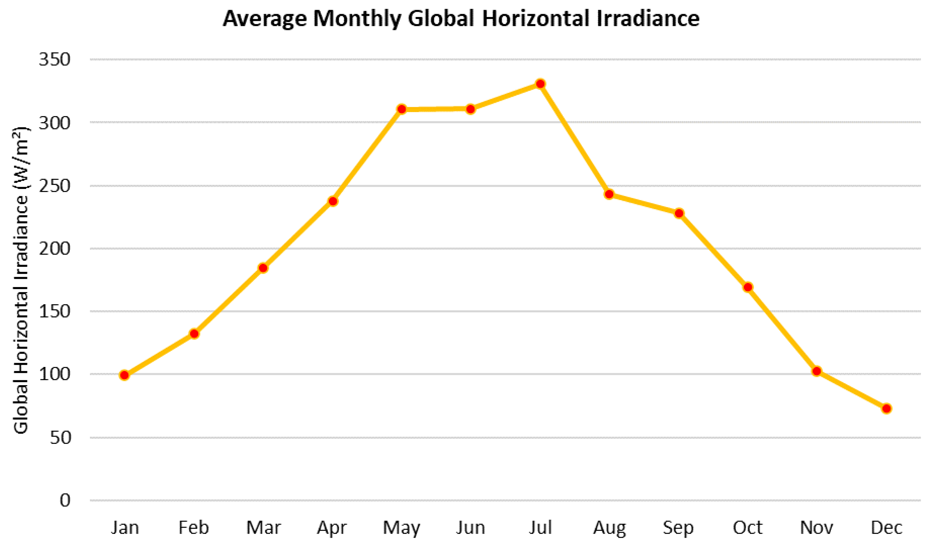
Figure 3.
Heatmap plot of the hourly spot price of electricity (Greece 2022, [23]).
Figure 3.
Heatmap plot of the hourly spot price of electricity (Greece 2022, [23]).
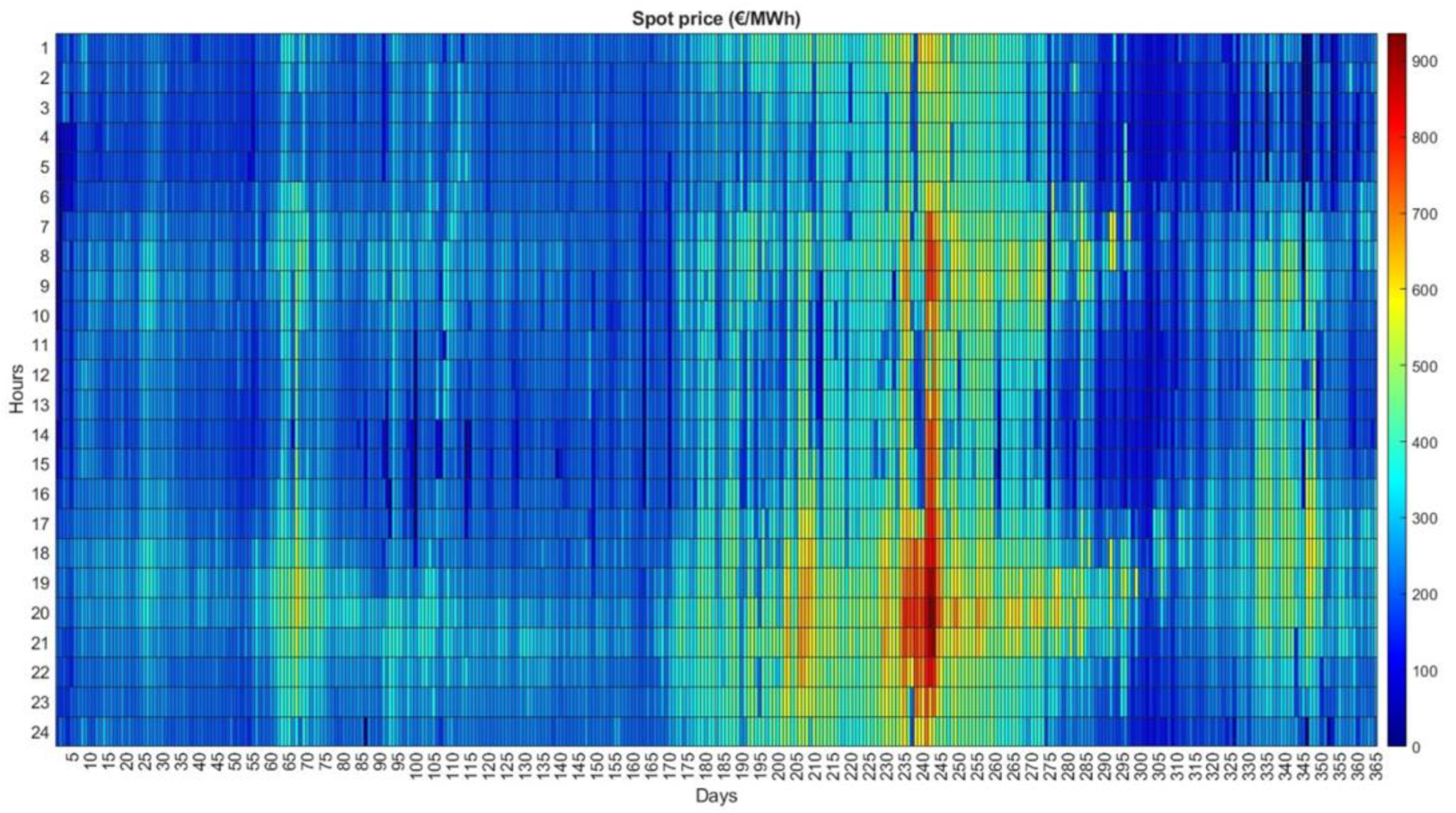
Figure 4.
Heatmap plot of the hourly CO2eq intensity of electricity (Greece 2022, [23]).
Figure 4.
Heatmap plot of the hourly CO2eq intensity of electricity (Greece 2022, [23]).

Figure 5.
Building D’ typical floor plan: (a). left side, and (b). right side.
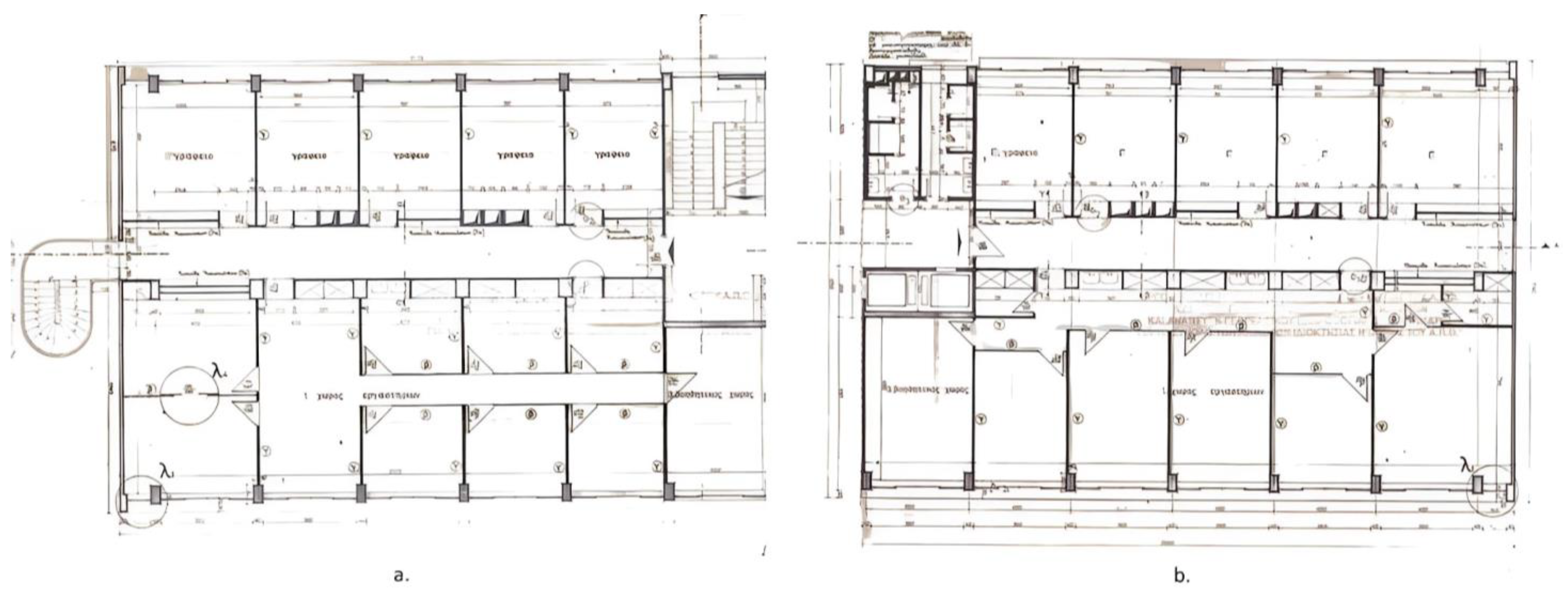
Figure 6.
Front (left) and 3D (right) view of the simulated building.

Figure 7.
Control scenario implementation for three consecutive days (case A building).
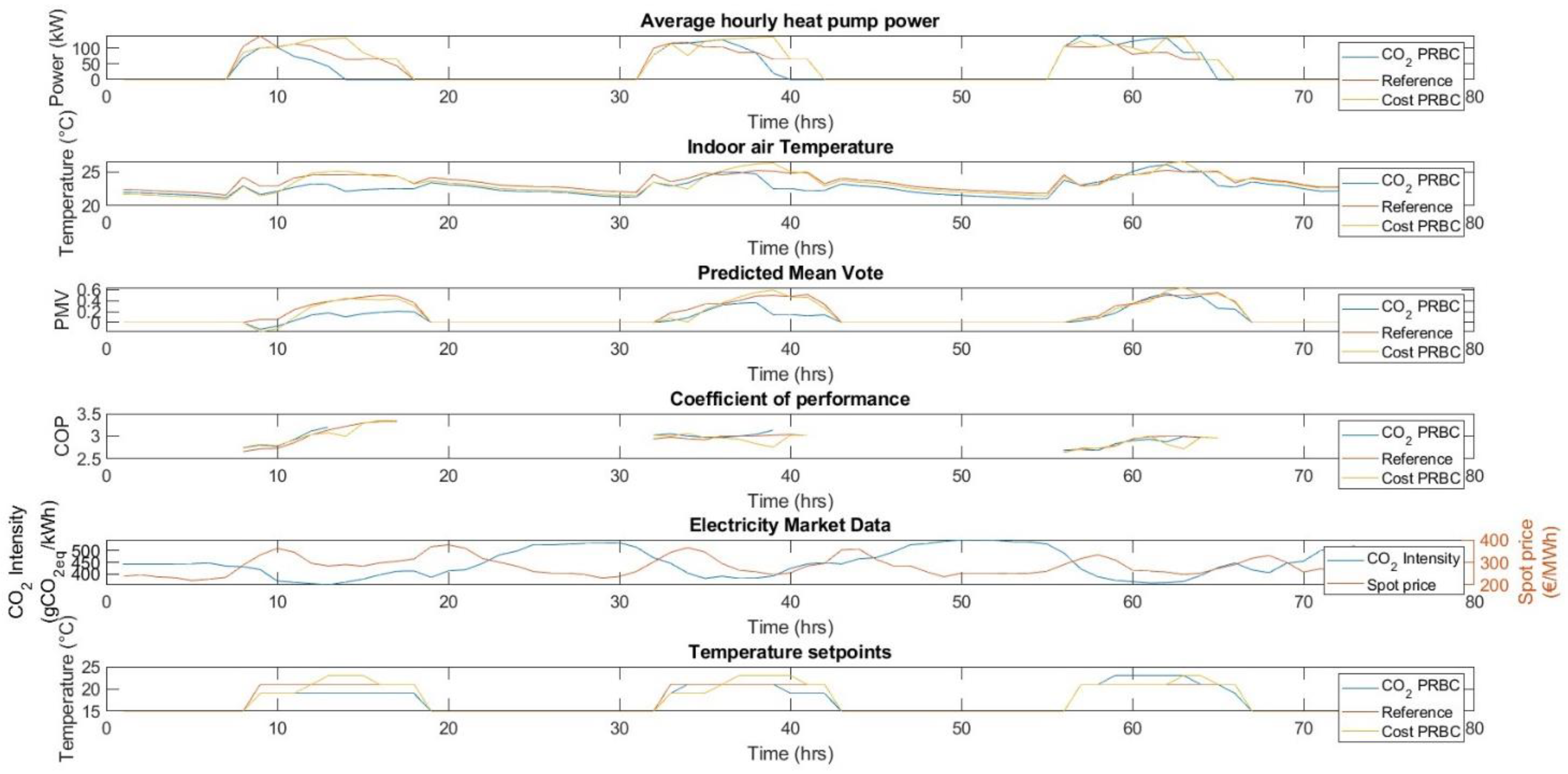
Figure 8.
Control scenario implementation for three consecutive days (reference building).

Figure 9.
Flexibility index in terms of cost.

Figure 10.
Flexibility index in terms of CO2eq.
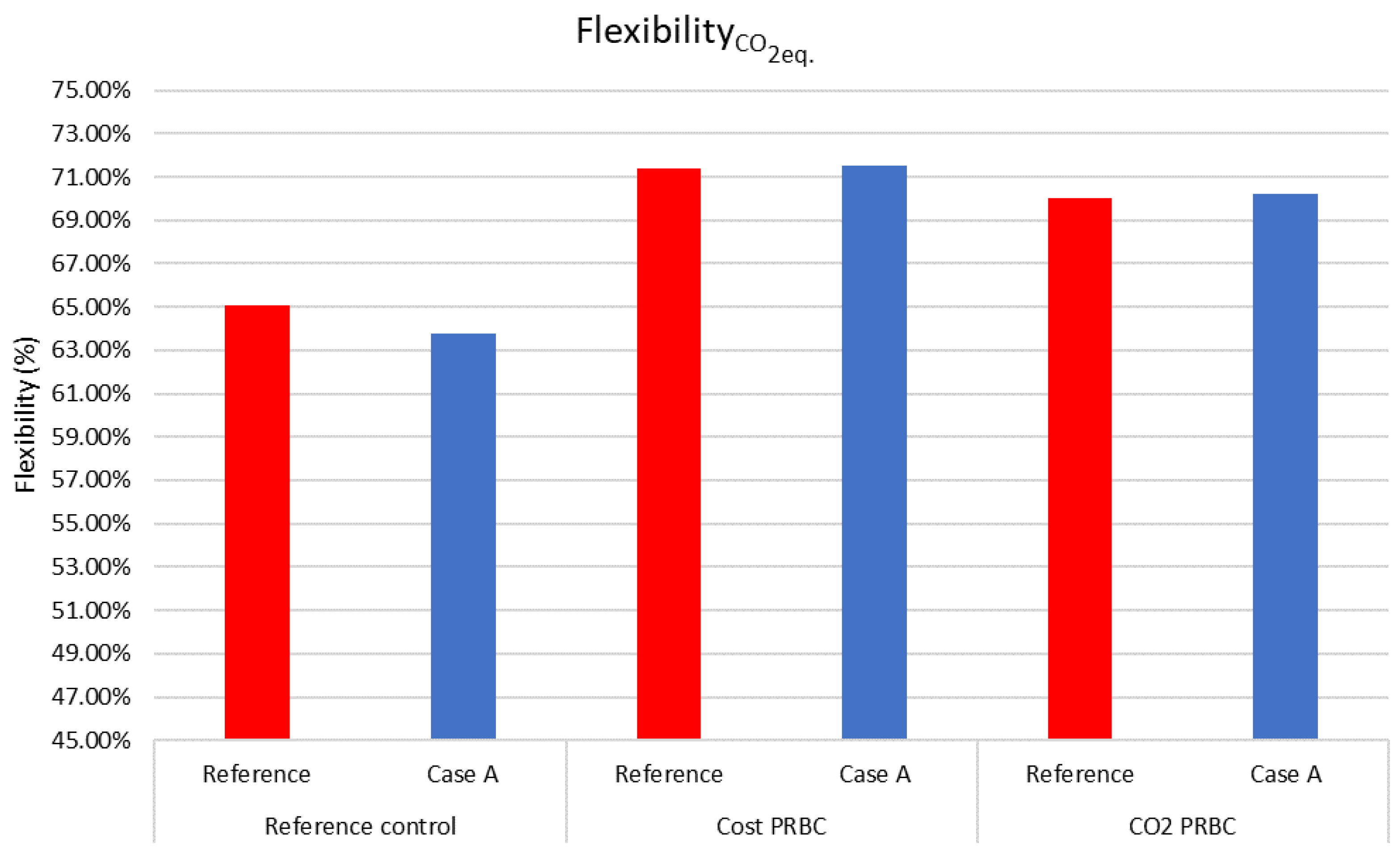
Figure 11.
Monthly electricity consumption for heating.
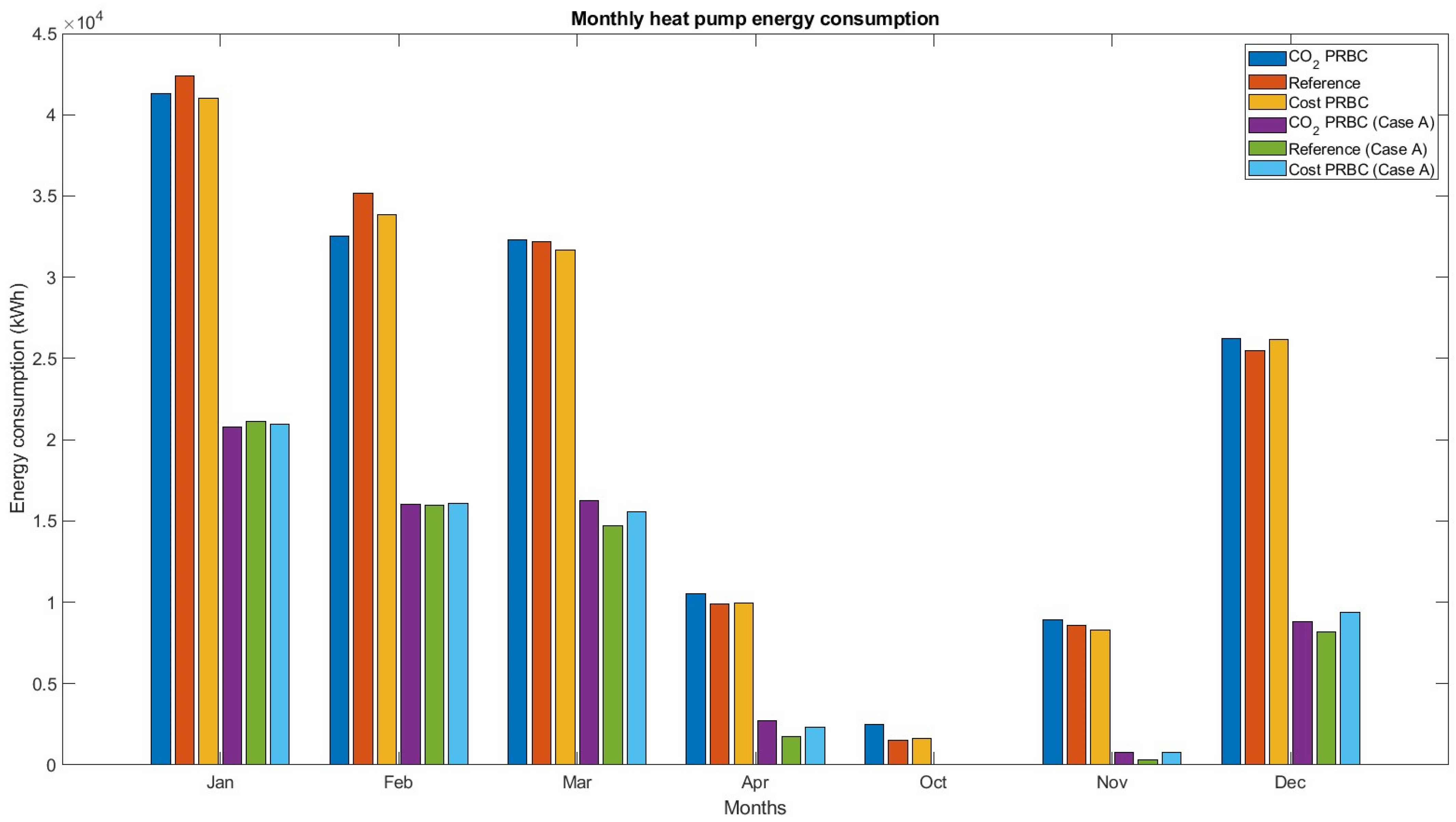
Figure 12.
Monthly energy costs for heating.

Figure 13.
Monthly CO2eq emissions for heating.


Table 1.
Internal operating conditions of thermal zones (imported from [29]).
Table 1.
Internal operating conditions of thermal zones (imported from [29]).
| Offices | Ancillary Spaces | |
|---|---|---|
| Working hours | 10 h/day | |
| Days of operation | 5 days/week | |
| Operating period | 12 months | |
| Heating setpoint | 21 °C | 18 °C |
| Number of users | 10 people/100 m2 | - |
| Fresh air required | 3 m3/h/m2 | 2.6 m3/h/m2 |
| Lighting level | 500 lx | 100 lx |
| Installed lighting power | 14 W/m2 | 2.8 W/m2 |
| People heat gain | 80 W/person | - |
| Equipment power | 15 W/m2 | - |
Table 2.
Thermal characteristics of the building shell.
| Component | Materials | U-Value (W/(m2K) | |
|---|---|---|---|
| Reference building | External walls | 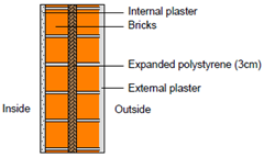 | 0.71 |
| Roof |  | 0.77 | |
| Ground floor |  | 3.11 | |
| Windows | double-glazed, aluminum frame | 2.82 | |
| Case A building | External walls |  | 0.35 |
| Roof | 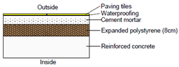 | 0.37 | |
| Ground floor |  | 3.11 | |
| Windows | Argon filler double-glazing, aluminum frame with thermal break | 1.57 |
Table 3.
Thermal mass flexibility evaluation.
| CADR | ηADR | |
|---|---|---|
| Unit | kWh | % |
| Reference | 115.6 | 43.9 |
| Case A | 121.9 | 53.2 |
Table 4.
Annual performance results.
| Energy | Costs | Emissions | Thermal Discomfort | ||||||
|---|---|---|---|---|---|---|---|---|---|
| Unit | kWh | % | EUR | % | CO2eq | % | h | % | |
| Reference building | Reference | 155,220 | - | 39,483 | - | 50,548 | - | 26 | - |
| Cost PRBC | 152,590 | −1.7% | 38,057 | −3.6% | 48,897 | −3.3% | 32 | 23.1% | |
| CO2 PRBC | 154,320 | −0.6% | 38,725 | −1.9% | 48,795 | −3.5% | 30 | 15.4% | |
| Case A building | Reference | 62,056 | - | 15,639 | - | 20,622 | - | 0 | |
| Cost PRBC | 65,119 | 4.9% | 15,747 | 0.7% | 20,839 | 1.1% | 0 | 0% | |
| CO2 PRBC | 65,299 | 5.2% | 16,089 | 2.9% | 20,599 | −0.1% | 0 | 0% | |
Disclaimer/Publisher’s Note: The statements, opinions and data contained in all publications are solely those of the individual author(s) and contributor(s) and not of MDPI and/or the editor(s). MDPI and/or the editor(s) disclaim responsibility for any injury to people or property resulting from any ideas, methods, instructions or products referred to in the content. |
© 2023 by the authors. Licensee MDPI, Basel, Switzerland. This article is an open access article distributed under the terms and conditions of the Creative Commons Attribution (CC BY) license (https://creativecommons.org/licenses/by/4.0/).
Share and Cite
MDPI and ACS Style
Chantzis, G.; Giama, E.; Papadopoulos, A.M. Building Energy Flexibility Assessment in Mediterranean Climatic Conditions: The Case of a Greek Office Building. Appl. Sci. 2023, 13, 7246. https://doi.org/10.3390/app13127246
AMA Style
Chantzis G, Giama E, Papadopoulos AM. Building Energy Flexibility Assessment in Mediterranean Climatic Conditions: The Case of a Greek Office Building. Applied Sciences. 2023; 13(12):7246. https://doi.org/10.3390/app13127246
Chicago/Turabian StyleChantzis, Georgios, Effrosyni Giama, and Agis M. Papadopoulos. 2023. "Building Energy Flexibility Assessment in Mediterranean Climatic Conditions: The Case of a Greek Office Building" Applied Sciences 13, no. 12: 7246. https://doi.org/10.3390/app13127246
Note that from the first issue of 2016, this journal uses article numbers instead of page numbers. See further details here.