
Optimal Path Planning and Tracking Control Methods for Parafoil

Academy of Astronautics, Nanjing University of Aeronautics and Astronautics, Nanjing 210016, China
*
Author to whom correspondence should be addressed.
Appl. Sci. 2023, 13(14), 8115; https://doi.org/10.3390/app13148115
Submission received: 30 April 2023
/
Revised: 8 July 2023
/
Accepted: 10 July 2023
/
Published: 12 July 2023
(This article belongs to the Section Aerospace Science and Engineering)
Abstract
:Due to the problems of flexible parafoil systems that are susceptible to complex disturbances, such as external wind fields and being difficult to control, it is necessary to study the path planning and tracking control methods of parafoil under complex conditions. In this paper, the particle model and dynamic model of the parafoil system are established, and the path planning method based on the original natural (ON) principle coupled with meteorological interference, terrain avoidance, and other environmental models is studied. Sliding mode control is introduced into the path tracking control of the parafoil system, and tracking errors of the parafoil position and velocity are taken as the design criteria for the sliding mode surface. The control law of the sliding mode controller is derived. Through simulation comparison with other path planning and tracking control methods, the methods designed in this paper can reflect better path planning and tracking performance. The methods designed in this paper can effectively suppress the impact of external disturbances, improve accuracy, and enhance robustness.
1. Introduction
As a new type of aircraft, the parafoil has the characteristics of high safety, simple operation, and stability. The parafoil system improves the safety and accuracy of the precision air drop, and makes up for the defects of the traditional circular parachute air drop system that flutters with the wind and has an uncontrollable landing point. It is an important part of the modern precision air drop system. The advanced precision air drop system uses a parafoil as the reducer, which has good controllability, and can achieve high altitude, long distance, and high-precision autonomous load delivery. It compensates for the shortcomings of the traditional air drop method, such as poor precision, target dispersion, and high risk, and greatly enhances the flexibility of air drop tasks.
The autonomous homing methods of the parafoil system mainly include simple homing, optimal control homing, and segmented homing. The segmented homing method has a higher engineering application value for parafoil systems with special flight characteristics. It is simple to implement and has higher stability and robustness. In view of the superior performance and broad application prospects of the parafoil system, the research on the parafoil system has not only urgent theoretical significance but also significant practical application value. However, when the inertial flight of the parafoil system is relatively stable, the control mechanism has poor sensitivity, a long time delay, and is more affected by the wind and other external environments. The control process is affected by the thrust and the external environment, which leads to local flexible deformation of the parachute and forms more complex nonlinear dynamic characteristics and coupling effects; when landing, it is required to achieve windward bird landing. All these put forward higher requirements for its modeling, path planning, and control. Therefore, to accurately homing the parafoil, it is necessary to further study the dynamic model, homing trajectory planning method, and the accurate control method of the parafoil in a complex environment.
Since the 1960s, relevant scholars have conducted a lot of research on the dynamics model of the parafoil system. Goodrick established the 3-DOF longitudinal plane model of the parafoil system based on the experimental data. In subsequent research, the parafoil body and the load of the parafoil system were regarded a rigid connected whole, and a 6-DOF rigid body model was established to analyze the flight performance and longitudinal stability of a small parafoil. The concept of added mass was first introduced into the model, making the model simulation results closer to the real experimental data [1,2,3]. Yang regarded the parachute body and the parachute rope as a rigid body in plane motion, and the load has a swing degree of freedom around the tether point, and established a longitudinal 4-DOF dynamic model of the dynamic parafoil to solve the dynamic response of the thrust step of the system from level flight to climbing state [4]. Mortaloni identified the unknown quantity in the added mass of the parafoil system by the parameter identification method and established a more accurate 6-DOF model [5]. Xiong established the dynamic model of the 6-DOF parafoil system, in which the aerodynamic force was selected by combining experimental data and engineering subsection processing; on this basis, the influence of different design parameters on the motion characteristics of the parafoil system was analyzed [6]. Muller equates the connection between the parachute body and the load of the parafoil system to two symmetrical suspension points, ignores the relative rolling motion between the two bodies, and establishes an 8-DOF dynamic model to study the relative yaw and pitch motion of the two bodies [7]. Xiong improved on Muller’s model and obtained a more perfect 8-DOF model [8]. Slegers further simplified the connection between the two bodies of the parafoil system into a hinge connection with certain constraints and established a 9-DOF dynamic model [9]. Visnyak regarded the two parts of the parafoil system as rigid bodies connected by elastic deformation slings, established a more complex 12-DOF nonlinear model for the parafoil system, and analyzed the dynamic characteristics of the parafoil system during turning and landing [10]. At the same time, Visnyak considered the influence factors of wind on the model.
Parafoil path planning requires that the specific path from the initial position to the target position that meets the performance index be planned under the condition that the parafoil landing requirements and the flight characteristics of the parafoil system are met. There are many algorithms that can be used for parafoil flight path planning. At present, the commonly used random landmark method, neural network algorithm, simulated annealing algorithm, genetic algorithm, particle swarm optimization algorithm, and ant colony optimization algorithms are random algorithms. Deterministic algorithms include the VORONOI diagram method, A * algorithm, and D * algorithm. Slegers transformed the optimal control problem in the upwind alignment phase of the parafoil system into a two-point boundary value problem for the solution [11]. Due to the complexity of the indirect method, the direct method is often used in the design of the homing trajectory of the parafoil system. Zhang and Gao used the Gaussian pseudospectral method to transform the discrete processing of the homing trajectory of the parafoil system into a large-scale nonlinear optimization problem with a series of algebraic constraints, and solved it with a quadratic programming method [12,13]. Xie studied the flight path of the parafoil system under terrain and fire threats, modeled the two threats, generated a three-dimensional search space, optimized the flight path of the parafoil system using a particle swarm optimization algorithm, and planned a homing path that can avoid threats and meet the range and height constraints [14]. Jiao used nonuniform B-spline technology to turn the trajectory planning problem into a parameter optimization problem, and combined with a chaotic particle swarm optimization algorithm to study the path planning problem of the parafoil air drop robot system in a disaster environment [15]. Pu studied the position control and direction control of the target approach section and energy constraint section, respectively, and proposed an angle control method that can be used for segmented homing of the parafoil system [16]. Zhang studied the path segmentation planning of the parafoil system under energy constraints using an improved particle swarm optimization algorithm [17]. Kaminer studied the sectional path planning of the parafoil air drop system with the help of optimal control theory, and designed a nonlinear trajectory tracking controller, which was finally verified by the simulation [18]. Liu improved the particle swarm optimization algorithm, improved the global search ability and speed of the algorithm, and applied it to the trajectory planning of the parafoil system [19]. Pini systematically studied the humanitarian material air drop rescue system in a disaster environment, introduced the system dynamics model, the generation of the homing trajectory and the navigation method, and designed a unified scheduling management mode for the flight of multiple parafoil systems [20]. Jiang transformed the constrained optimal control problem into an unconstrained optimal control problem based on the principle of control variable parameterization method and the precise optimization algorithm of penalty functions, and solved it using Sequential Quadratic Programming (SQP) [21]. Tao adopted a genetic algorithm with an elite strategy to optimize the homing path and introduced the static penalty function method with a relaxation factor to deal with inequality constraints [22]. Zhao adopted the design scheme of the sub-section homing based on the four-degrees-of-freedom model and optimized the design parameters of the homing trajectory using the improved Artificial Fish-Swarm Algorithm (AFSA) [23]. Gao took the minimum homing energy consumption as the optimization goal, adopted a five-segment homing strategy, used the pseudospectrum method to optimize the trajectory, and gave the optimal reference path for homing [24]. Zhang proposed a 3D trajectory planning method based on a compound optimization random tree (CO-RRT) algorithm for parafoil trajectory planning under specific conditions [25].
Tracking control is the key link to achieving accurate autonomous positioning of the parafoil system. Based on the analysis of existing literature, the traditional control methods of the parafoil system mainly focus on PID, model predictive control, and nonlinear dynamic inversion. Other robust control methods such as fuzzy control and intelligent control combined with optimization methods have also been studied in the field of parafoil tracking control. Xiong studied the trajectory tracking problem of the parafoil system in the Serret Frenet coordinate system and adopted the proportional differential (PD) control algorithm as the trajectory tracking controller [26]. The simulation results verify the feasibility of the method. Hu used the traditional PID control method to control the parafoil by establishing a 9-DOF model [27]. Qian proposed a control method that combined neural network and dynamic inversion control for autonomous parafoil flight control, aiming to eliminate the difficulty of establishing an accurate dynamic model of the parafoil system, and the effectiveness of the algorithm was verified by simulation [28]. Xie proposed a nonlinear predictive control method based on fuzzy disturbance observer and applied it to the trajectory tracking control of the parafoil system [29]. Zhu designed a fuzzy controller for the trajectory tracking of the parafoil system and achieved a better control effect than the traditional PID control method [30]. Li further proposed an adaptive controller based on the error-switching fuzzy control algorithm and the generalized predictive control algorithm in the tracking process [31]. Culpepper studied the control problem of the parafoil system in case of failure and proposed a control logic with the adaptive capability to deal with the possible damage of the parachute jacket or the twining of the parafoil rope in the parafoil system [32]. Rademacher introduced the navigation, guidance, and control of the parafoil system, proposed an online trajectory planning method and a trajectory error calculation method, and designed a proportional control rate to eliminate the trajectory error [33,34]. Benjamin applied the adaptive control method to the tracking control of large parafoils [35]. In the actual parafoil air drop application, the ALEX parafoil air drop system uses a simple proportional controller for homing control [36]. Tao designed the flight guidance rate using the 2D trajectory tracking strategy based on guidance and used the Linear Active Disturbance Rejection Control (LADRC) strategy to correct the trajectory tracking error in real time, improving the anti-interference ability and robustness of the parafoil system [37]. Sun proposed a trajectory tracking controller based on ADRC combined with PID control [38]. Garcia proposed two passivity-based control (PBC) algorithms to control an unmanned powered parallel aerial vehicle and compared their performance [39]. Hanafy designed a fuzzy logic controller (FLC) to control the lateral motion of powered parachute (PPC) flying vehicles and used a genetic algorithm (GA) to optimize the fuzzy membership functions [40]. Carlos addresses the issue of the parachute not being able to return to its equilibrium position due to control locking caused by excessive control [41]. He used the method of multi-body simulation to study the occurrence of locking phenomena and provided passive methods to avoid instability. In addition, the simulation results were also used to demonstrate that active control using parachute brake input can avoid the occurrence of locking instability. Cacan studied the uncertainty problem of system flight dynamic response when the wind speed exceeds the airspeed of the parafoil flight, and proposed a direct and indirect combination of adaptive control strategies to quickly describe the dynamic characteristics of the parafoil [42]. This algorithm can achieve high-precision landing under various degradation conditions. Garcia proposed two passivity-based control (PBC) algorithms to control an unmanned powered parallel aerial vehicle, and compared their performance. Hanafy designed a fuzzy logic controller (FLC) to control the lateral motion of powered parachute (PPC) flying vehicles, and used a genetic algorithm (GA) to optimize the fuzzy membership functions.
In this paper, we introduced the current research status of parafoil dynamics modeling, homing path planning, and path tracking control. We mainly discuss path planning and tracking control for parafoil based on the original natural (ON) algorithm and sliding mode control (SMC). The flight path planning method designed in this paper can be used to plan an optimal flight path from the starting point to the landing point of the parafoil and meet the performance constraints of the parafoil, the initial position and terminal position, and the heading constraints. Using the tracking control method designed in this paper, the parafoil can follow the planned optimal path within the error range. Simulation comparisons with other methods can indicate that the methods designed in this paper can achieve better parafoil flight performance under complex conditions, thereby verifying the rationality of the design methods. The research work carried out in this paper on parafoil air drop systems provides reference ideas and a theoretical basis for actual air drop projects and has certain theoretical significance and engineering value.
2. Model of Parafoil
The aerodynamic shape of the parafoil determines the aerodynamic force and aerodynamic moment of the parafoil vehicle, and changes the flight performance of the parafoil accordingly. After inflation, the parafoil is fully deployed, and its basic structural parameters are shown in Figure 1.
The basic parameters of the parafoil structure mainly include the following parts:
Span b: the spanwise length of the fully deployed parafoil.
Chord length c: chordal length of fully deployed parafoil.
Aspect ratio : , S is the horizontal projected area of the canopy. For a rectangular parafoil, .
Air-cell height : the longest distance between the upper and lower chords of the front edge of the canopy.
Installation angle : the angle between the reference chord length of the wing profile and the horizontal line when the parafoil glides in balance. Once the rope length is determined, can also be determined. changes with the rope length and varies with different parafoil.
Attack angle : the angle between the opposite direction of the air and the lower wing surface in the longitudinal plane.
The values of the basic parameters of the parafoil structure are not fixed and unique. It is necessary to select appropriate structural parameters according to the dynamic characteristics of the parafoil air-drop system and the laws of control.
is the symmetric downward bias and is the asymmetric downward bias, which is obtained from the parameters shown in Figure 2. The range of values of d is 0 to 0.24c. The symmetric downward bias , the value range is 0 to 1. The asymmetric downward bias , the value range is 0 to 0.24, where 0 corresponds to no asymmetric downward bias and 0.24 corresponds to complete unilateral downward deviation. b is the wingspan, and c is the length of the chord. , , represent the projections of the parafoil angular velocity on the x, y, and z components of the body coordinate system, and , , represent the projections of the parafoil velocity on the x, y, and z components of the body coordinate system. is the parafoil velocity. is the attack angle and is the side-slip angle. , , and are obtained by interpolating the relevant subject data, and other coefficients are fixed values [43], as shown in Table 1. The expression of parafoil moment of inertia is shown in Equations (A12)–(A15) in Appendix A.
The particle dynamics equation of the parafoil system and the dynamics equation of the parafoil system rotating around the particle are shown in Equations (1) and (2). The particle kinematics equation of the parafoil system and the kinematics equation of the parafoil system rotating around the particle are shown in Equations (3) and (4).
where, L, D, and Y are the lift, drag, and lateral force of the parafoil, respectively. and are the inclination and deflection of the flight path, respectively. , , and are pitch angle, yaw angle, and tilt angle, respectively. , , and are components of rotational angular velocity on each axis of the body coordinate system. , , and are the rotational inertia of each axis in the body coordinate system. is the inertia product of the axis in the body coordinate system.
The parafoil system is a complex multi-body model with high nonlinearity and strong coupling. However, for the study of the homing trajectory of the parafoil system, it is often not necessary to study the attitude change of the system in space, but only the position change of the system in space. Therefore, a simple particle model is usually used in the trajectory planning problem. Based on the ground coordinate system, the target point of trajectory planning is regarded as the coordinate origin, and the simplified particle model expression of the parafoil system motion equation is obtained as shown in Equation (5).
where, is the horizontal flight velocity and is the vertical falling velocity. and , respectively, represent the projection of horizontal wind velocity on the X and Y axes. u represents the control quantity, and its value range is . is the maximum control quantity allowed to be input. The value of u is related to the unilateral downward deflection of the control rope of the parafoil system, and the two are in one-to-one correspondence, and the value of u is the largest when the turning radius is the smallest.
Comparing a semi-ellipsoidal sphere to a threat peak, assuming that there are k semi-ellipsoidal threat areas in the flight environment, and taking the terrain height value as the threat coefficient, the terrain threat model is as follows.
where, represents the actual terrain height at this location, represents the central coordinate position of the ith threat peak, represents the attenuation coefficient of the ith threat peak in the X-axis and Y-axis directions, and represents the height of the ith threat peak.
3. Optimal Parafoil Path Planning Method
The original natural principle has universality, and numerical algorithms based on this principle are applicable to the integrated global optimization design of dynamic control and decision making for many primitive material units, many levels, and many types of material combinations in unknown random environments [44]. In this paper, we designed a parafoil path planning method based on the original natural principle to solve the parafoil optimal path planning problem. This method is used to generate a 4D flight path, that is, the selected path segment is connected into a nearly complete 4D path. To maintain flexibility and reduce the number of paths, in this step, the starting navigation point and the target are not temporarily connected to the track. The most basic algorithm used here is the shortest path algorithm based on original natural principles, which is an extremely effective method of extracting a group of track segments to minimize the cost of the track between the initial navigation point and the final pair of navigation points. Each starting navigation point can eventually reach many other navigation points. Therefore, the result of the algorithm is actually represented as a tree. This tree contains the best route from each starting navigation point to each terrain-matching point it can reach. In this way, the overflight cost of each route of each tree can be obtained and stored.
Without considering the effect of interference sources, the discrete description of the optimal control problem of the parafoil system is simplified, and the simplified nonlinear discrete system state equation is obtained.
where the state constraint and the control constraint . It is necessary to find the optimal control sequence so that the following cost functions reach the minimum.
The calculation steps based on the original natural algorithm are as follows.
: Calculate the optimal control of the level and obtain the following equation.
Then, we can calculate , and .
: Calculate the optimal control of the level.
Then, we can calculate , and .
…
: Calculate the optimal control of the kth level.
Then, we can calculate , and .
…
: Calculate the optimal control of the Nth level.
Then, we can calculate , and .
: This is the last step. Calculate the natural performance index , natural control , and state variable in order from the starting point , where k ranges from 1 to N.
4. Optimal Flight Path Tracking Control Method for Parafoil
Flight path tracking control means that when the system gives a planned path, the parafoil can fly along the given path according to its own flight characteristics and maximum control range. Sliding mode control can effectively overcome the uncertainty of parafoil systems. The control algorithm has the advantages of simple form, fast response speed, and good control effect for nonlinear systems. At present, traditional PID control is widely used in the tracking control of the parafoil system. The introduction of sliding mode control will provide a new solution for the control of the parafoil system.
The path tracking method used in this paper is to track a given path by designing a tracking control law based on sliding mode control, using a fixed point on a path that is a certain distance from the system location as a reference point on the planned desired path, and controlling the parafoil to fly with this series of reference points as the target. The simple flow of the tracking control method is shown in Figure 3.
In the parafoil system, the conversion between the dynamic model and the kinematic model involves the conversion of some aerodynamic parameters, which are shown in Appendix B.
Define the position error and the velocity error as shown in Equation (13), and the sliding surface design as shown in Equation (14).
The derivative of Equation (5) can be obtained as follows.
The derivative of s is as follows.
The expression of can be obtained as follows.
where we replace the turning angular velocity with u as the control input to the parafoil dynamics model.
Define the exponential approach law as follows.
Define the Lyapunov function and take its derivative as follows.
According to Equation (19), the designed sliding surface meets the Lyapunov stability criterion.
5. Simulation Results and Analysis
5.1. Path Planning for Parafoil
According to the glide ratio constraints of the parafoil system, the maximum drop height of the parafoil system is limited to 7 km and the maximum horizontal drop distance is 40 km. Assuming that the initial position of the parafoil system is [0, 17.5, 6.5] km and the initial flight direction is 90 degrees, the homing flight trajectory of the parafoil system typically requires gliding for a distance along the initial flight direction. The wind speed of the wind field in the ground coordinate system is 10 m/s. The coordinates of the landing position are [40, 0, 0] km. In the simulation verification stage of this study, we established various distributed terrains and threat areas, as well as various wind fields in different directions and forms. Finally, we chose a more complex form of terrains and threat areas as shown in Figure 4, and three typical forms of wind fields as shown in Figure 5, Figure 6 and Figure 7, which are rotational wind field, crosswind field, and headwind field. The specific simulation conditions for parafoil path planning are shown in Table 2.
Figure 4 shows the threat areas simulated with a cylindrical surface and the terrains simulated with a quadric surface, such as mountains at different heights. During the parafoil flight, it should bypass the threat areas and cross the terrains at a safe altitude. Figure 5, Figure 6 and Figure 7 show three different forms of wind field to simulate the impact of different external environments on parafoil flight.
Figure 8, Figure 9 and Figure 10 show the comparison between the parafoil flight path planned by the path planning method based on the original natural(ON) algorithm designed in this paper and the parafoil flight path planned by the compound optimization random tree (CO–RRT) algorithm used in Ref. [25]. CO–RRT is an incremental search method based on sampling, which is a single query algorithm. The flight range of the parafoil flight path planned by the ON algorithm is 4.65 km, and the flight time is 968.8 s. The flight range of the parafoil flight path planned by the CO–RRT algorithm is 4.69 km, and the flight time is 1090.1 s. It can be seen that the parafoil flight path planned by the ON algorithm has a shorter range and flight time, whereas the velocity and acceleration trends planned by the two algorithms are similar, which means that under the same flight constraints, using the ON algorithm can plan a better parafoil flight path.
Figure 11, Figure 12 and Figure 13 show the comparison of the planned paths, planned velocities, and planned accelerations of the parafoil under three different wind field conditions.It can be seen that the flight time of a parafoil under the influence of a rotating wind field is significantly longer than that of a crosswind field and an upwind field. This is because the direction of the wind changes at each moment when the parafoil passes through the rotating wind field, which requires both the use of wind field flight and resistance to wind field influence to be considered when planning the parafoil path. This also makes the planned parafoil flight path unstable, thereby extending the flight time. It is illustrated that under the constraints of the shortest distance, the shortest time, and the minimum turning radius, the algorithm studied in this paper can make full use of the wind fields to plan the optimal path.
5.2. Path Tracking for Parafoil
The path tracking simulation of parafoil is based on the planned path shown in Figure 8. The initial path inclination and deflection of the parafoil are both 0 degrees. The sliding mode control(SMC) method designed in this paper and the tracking control method combining active disturbance rejection control(ADRC) and PID control used in Ref. [38] are used to track the planned path of the parafoil, respectively. The ADRC–PID method proposed can estimate and compensate the system modeling error and nonlinear uncertainty disturbance through the extended state observer. The specific simulation conditions for parafoil path tracking are shown in Table 3. A series of comparative simulations are performed in the following.
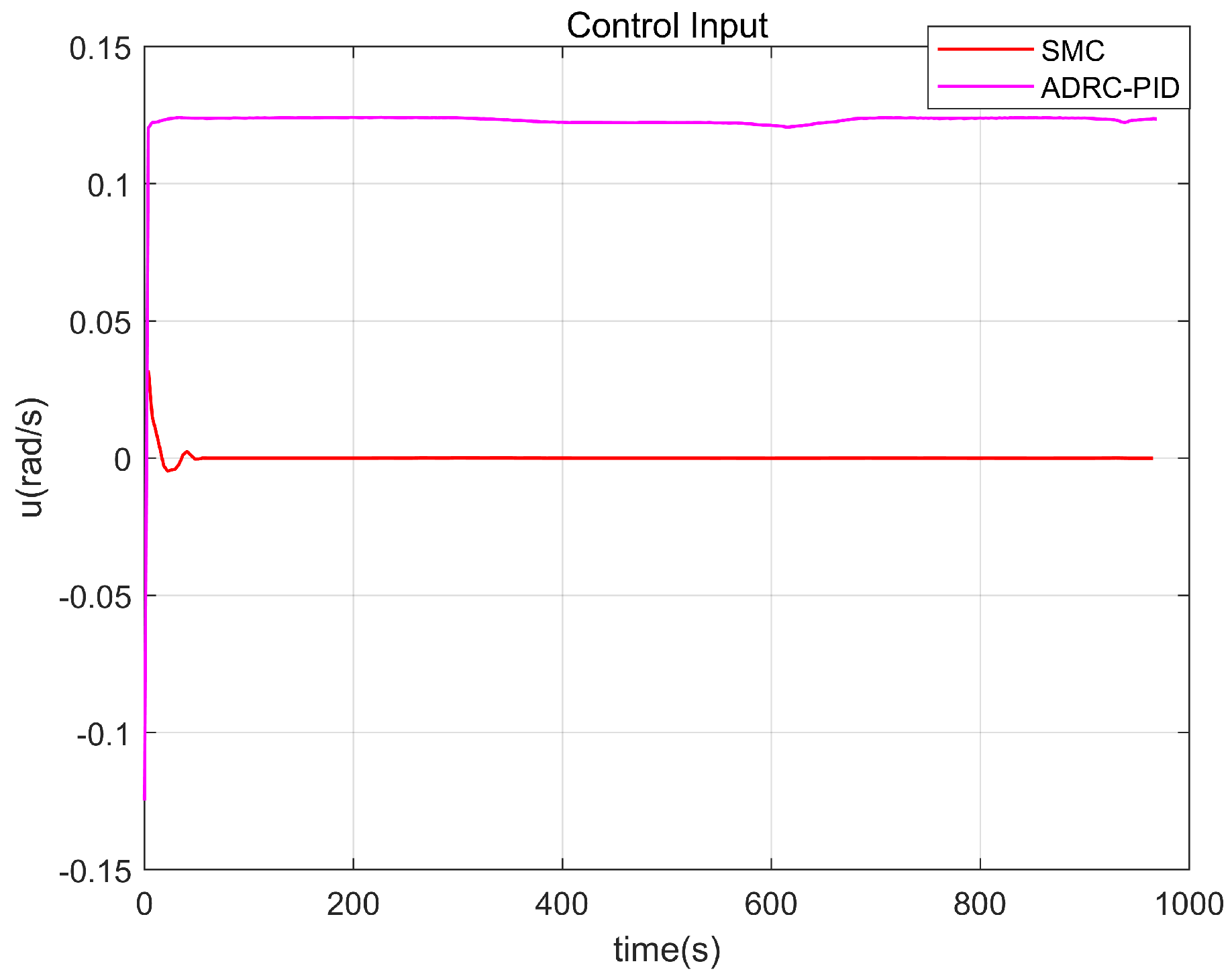
Figure 14 shows the parafoil path tracking using the sliding mode tracking control method designed in this paper, and Figure 15 shows the parafoil path tracking using the ADRC–PID method. Figure 16 and Figure 17 show the velocity tracking and acceleration tracking of the parafoil under the two tracking methods, respectively. From the comparison in Figure 16, it can be seen that the parafoil velocities tracked by SMC can better fit the planned velocities and the tracking error is smaller. From the comparison in Figure 17, the SMC tracking method also has better tracking performance for parafoil acceleration. Figure 18 shows the path tracking errors under the two tracking methods. Figure 19 shows the control input on the path tracking process for parafoil under the two tracking methods. From Table 4, it can be seen that although the SMC method has a higher maximum error in tracking the parafoil flight path, the average errors are less than the average errors of the ADRC–PID method, which can indicate that the SMC method designed in this article has better tracking performance for the parafoil flight process.
6. Conclusions
In this paper, we mainly study the path planning and path tracking control of the parafoil system and simulated the design method in various situations based on 6-DOF parafoil model. Compared to the CO–RRT method, it can be seen that the path planning method based on the original natural algorithm has better planning performance and can plan a better parafoil path. This method can quickly plan the optimal flight path of the parafoil system under random external conditions, which shows the reliability of the method. The parafoil path tracking control method based on the sliding mode control theory studied in this paper can accurately track the planned optimal path, reach the target point within the error range, track the parafoil velocity and acceleration commands well, and control the error within the controllable range. Compared with the ADRC-PID method, it can be seen that the SMC based path tracking method has better tracking performance and achieves higher tracking accuracy.
In this paper, we have achieved certain results in our research on parafoil systems, the following aspects can still be further studied in the future:
(1) In the selection of aerodynamic parameters, a more accurate aerodynamic database can be established.
(2) Realizing precise air drop of parafoil systems is a complex problem. This article only focuses on the precise air drop under constant wind conditions. The actual engineering wind field model is complex and variable, and further refinement of the wind field model is needed.
(3) SMC has significant fluctuations in the initial stage of control, which means that the system generates chattering and can further reduce the degree of chattering.
Author Contributions
Conceptualization, Z.L.; methodology, Z.L.; software, Z.L.; validation, Z.L. and Y.N.; formal analysis, Z.L.; investigation, Z.L.; resources, Z.L.; data curation, Y.N.; writing—original draft preparation, Z.L.; writing—review and editing, Y.N.; visualization, Z.L.; supervision, Y.N.; project administration, Y.N.; funding acquisition, Y.N. All authors have read and agreed to the published version of the manuscript.
Funding
This research was funded by Project of the Aviation Science Foundation of China [No. 201929052002].
Data Availability Statement
Sample data available on request.
Conflicts of Interest
The authors declare no conflict of interest. The funders had no role in the design of the study; in the collection, analyses, or interpretation of data; in the writing of the manuscript, or in the decision to publish the results.
Nomenclature
| b | Span of parafoil |
| c | Chord length of parafoil |
| Aspect radio | |
| Air-cell height | |
| Attack angle and sideslip angle | |
| Air density | |
| S | Reference area |
| Umbrella area | |
| m | Parafoil mass |
| P | Dynamic pressure |
| Lift, drag, and side force | |
| Lift, drag, and side force coefficient | |
| Axial force coefficient | |
| Roll, pitch, and yaw moment | |
| Roll, pitch, and yaw moment coefficient | |
| Symmetric downward bias of parafoil | |
| Asymmetric downward bias of parafoil | |
| Asymmetric control drag coefficient | |
| Asymmetric control lift coefficient | |
| sideslip angle induced Y-axis force coefficient | |
| Asymmetric control induced Y-axis force coefficient | |
| Y-axis aerodynamic coefficient induced by rotation about the Z-axis | |
| sideslip angle induced X-axis moment coefficient | |
| Asymmetric control induced X-axis moment coefficient | |
| X-axis moment coefficient induced by rotation about the X-axis | |
| X-axis moment coefficient induced by rotation about the Z-axis | |
| sideslip angle induced Z-axis moment coefficient | |
| Asymmetric control induced Z-axis moment coefficient | |
| Z-axis moment coefficient induced by rotation about the X-axis | |
| Z-axis moment coefficient induced by rotation about the Z-axis | |
| Asymmetric control induced Y-axis moment coefficient | |
| Y-axis moment coefficient induced by rotation about the Y-axis | |
| Velocity of parafoil | |
| Horizontal velocity of parafoil | |
| Projections of parafoil velocity on the body coordinate system | |
| Projections of tracking target on the body coordinate system | |
| Flight path inclination and deflection | |
| Position of parafoil on the earth coordinate system | |
| Rotational angular velocity | |
| Components of on the X, Y, and Z axes | |
| Pitch angle, yaw angle, and roll angle | |
| Yaw angle rate | |
| u | Control input |
Appendix A
Appendix B
References
- Goodrick, T.F. Theoretical study of the longitudinal stability of high performance gliding air drop systems. In Proceedings of the 5th Aerodynamics Deceleration Systems Conference, Albuquerque, NM, USA, 17–19 November 1975. [Google Scholar]
- Goodrick, T.F. Comparison of simulation and experimental data for a gliding parachute in dynamic flight. In Proceedings of the 7th Aerodynamic Decelerator and Balloon Technology Conference, San Diego, CA, USA, 21–23 October 1981. [Google Scholar]
- Goodrick, T.F. Scale effects on performance of ram air wings. In Proceedings of the 8th Aerodynamic Decelerator and Balloon Technology Conference, Hyannis, MA, USA, 2–4 April 1984. [Google Scholar]
- Yang, H.; Song, L.; Wang, W.J. 4-DOF longitudinal dynamic simulation of powered-parafoil. J. Beijing Univ. Aeronaut. Astronaut. 2014, 40, 1615–1622. [Google Scholar]
- Mortaloni, P.A.; Yakimenko, O.A.; Dobrokhodov, V. On the development of a six-degree-of-freedom model of a low-aspect-ratio parafoil delivery system. In Proceedings of the 17th AIAA Aerodynamic Decelerator Systems Technology Conference and Seminar, Monterey, CA, USA, 19–22 May 2003. [Google Scholar]
- Xiong, J.; Qin, Z.Z.; Wen, H.W. Optimal Control of Parafoil System Homing. Aerosp. Control 2004, 22, 32–36. [Google Scholar]
- Muller, S.; Wagner, O.; Sachs, G. A high-fidelity nonlinear multibody simulation model for parafoil systems. In Proceedings of the 17th AIAA Aerodynamic Decelerator Systems Technology Conference and Seminar, Monterey, CA, USA, 19–22 May 2003. [Google Scholar]
- Xiong, J.; Song, X.M.; Qin, Z.Z. Analysis on Two Body Relative Movement of Parafoil System. Spacecr. Recovery Remote Sens. 2004, 25, 10–16. [Google Scholar]
- Slegers, N.J. Effects of canopy-payload relative motion on control of autonomous parafoils. J. Guid. Control Dyn. 2010, 3, 116–125. [Google Scholar] [CrossRef]
- Vishnyak, A. Simulation of the payload-parachute-wing system flight dynamics. In Proceedings of the Aerospace Design Conference, Irvine, CA, USA, 16–19 February 1993. [Google Scholar] [CrossRef]
- Slegers, N.J.; Yakimenko, O. Optimal control for terminal guidance of autonomous parafoils. In Proceedings of the 20th the AIAA Aerodynamic Decelerator Systems Technology Conference and Seminar, Seattle, WA, USA, 4–7 May 2009. [Google Scholar]
- Zhang, L.; Gao, H.; Chen, Z.; Sun, Q.; Zhang, X. Multi-objective global optimal parafoil homing trajectory optimization via Gauss pseudo spectral method. Nonlinear Dyn. 2013, 72, 1–8. [Google Scholar] [CrossRef]
- Gao, H.; Zhang, L.; Sun, Q.; Sun, M.W.; Chen, Z.Q.; Kang, X.F. Fault-tolerance design of homing trajectory for parafoil system based on pseudo-spectral method. Control Theory Appl. 2013, 30, 702–708. [Google Scholar]
- Xie, Y.; Wu, Q.X.; Jiang, C.S.; Zheng, C. Application of Particle Swam Optimization Algorithm in Route Planning for Parafoil Airdrop System. Aero Weapon. 2010, 5, 7–10. [Google Scholar]
- Jiao, L.; Sun, Q.L.; Kang, X.F. Route Planning for Parafoil System Based on Chaotic Particle Swarm Optimization. Complex Syst. Complex. Sci. 2012, 9, 47–54. [Google Scholar]
- Pu, Z.G.; Li, L.C.; Tang, B.; Zhang, Y. Segmental homing direction control method for parafoil system. J. Ordnance Equip. Eng. 2009, 30, 117–119. [Google Scholar]
- Zhang, X.H.; Zhu, E.L. Design and Simulation in the Multiphase Homing of Parafoil System Based on Energy Confinement. Aerosp. Control 2011, 29, 43–47. [Google Scholar]
- Kaminer, I.I.; Yakimenko, O.A. On the development of GNC algorithm for a high-glide payload delivery system. In Proceedings of the 42nd IEEE Conference on Decision and Control, Maui, HI, USA, 1–4 October 2003. [Google Scholar]
- Liu, Z.; Kong, J. Path planning of parafoil system based on particle swarm optimization. In Proceedings of the 2009 International Conference on Computation Intelligence and Natural Computing, Beijing, China, 6–7 June 2009. [Google Scholar]
- Pini, G.; Sharoni, F. Coordination and communication of cooperative parafoils humanitarian aid. IEEE Trans. Aerosp. Electron. Syst. 2010, 46, 1747–1760. [Google Scholar]
- Jiang, H.C.; Liang, H.Y.; Zeng, D.T.; Jin, Y. Design of the optimal homing trajectory of a parafoil system considering threat avoidance. J. Harbin Eng. Univ. 2016, 37, 955–962. [Google Scholar]
- Tao, J.; Sun, Q.; Zhu, E.; Chen, Z.; He, Y. Genetic algorithm based homing trajectory planning of parafoil system with constraints. J. Cent. South Univ. Sci. Technol. 2017, 48, 404–410. [Google Scholar]
- Zhao, Z.H.; Zhao, M.; Chen, Q.; Cai, L.J. Design in Multiphase Homing of 4- DOF Parafoil System Based on Improved Artificial Fish- Swarm Algorithm. Fire Control Command. Control 2017, 42, 64–68. [Google Scholar]
- Gao, F.; Guo, R.; Feng, Z.; Jie, J.; Zhang, Q. Optimization Design of Homing Trajectory of Parafoil System with Five Segments. Acta Armamentarii 2020, 41, 1025–1033. [Google Scholar]
- Zhang, H.; Meng, X.J.; Chen, Z.L.; Zhang, Y.; Liu, Z. Trajectory Planning in Three Dimensions for Unmanned Parafoil Based on Compound Optimization RRT. J. Command. Control 2022, 8, 235–238. [Google Scholar]
- Xiong, J.; Cheng, W.K.; Qin, Z.Z. Trajectory tracking control of parafoil system based on Serret-Frencet coordinate system. J. Dyn. Control 2005, 3, 87–91. [Google Scholar]
- Hu, W.Z.; Chen, J.P.; Zhang, H.Y.; Tong, M.B. Dynamic Modeling and Flight Control Simulation of Parafoil Aerial Delivery Systems. Aeronaut. Comput. Tech. 2017, 47, 70–73. [Google Scholar]
- Qian, K.C.; Chen, Z.L.; Li, J. Autonomous Flight Control Method of Powered Paraglider Based on Dynamic Inversion. Control Eng. China 2011, 18, 178–180. [Google Scholar]
- Xie, Y.R.; Wu, Q.X.; Jiang, C.S. Trajectory Tracking of Parafoil Using FDO Based Nonlinear Predictive Control. Electron. Opt. Control 2011, 18, 72–76. [Google Scholar]
- Zhu, E.L.; Zhang, X.H. Design and application of fuzzy controller in parafoil airdrop system. Electron. Meas. Technol. 2011, 34, 46–49. [Google Scholar]
- Li, Y.X.; Chen, Z.Q.; Sun, Q.L. Flight path tracking of a parafoil system based on the switching between fuzzy control and predictive control. CAAI Trans. Intell. Syst. 2012, 7, 1–8. [Google Scholar]
- Culpepper, S.; Ward, M.B.; Costello, M.; Bergeron, K. Adaptive control of damaged parafoils. In Proceedings of the 22nd AIAA Aerodynamic Decelerator Systems (ADS) Conference, Daytona Beach, FL, USA, 25–28 March 2013. [Google Scholar]
- Rademacher, B.; Lu, P.; Strahan, A.; Cerimele, C. Trajectory design, guidance and control for autonomous parafoils. In Proceedings of the AIAA Guidance, Navigation and Control Conference and Exhibit, Honolulu, HI, USA, 18–21 August 2008. [Google Scholar]
- Rademacher, B.J.; Lu, P.; Strahan, A.L.; Cerimele, C.J. In-flight trajectory planning and guidance for autonomous parafoils. J. Guid. Control Dyn. 2009, 32, 1697–1712. [Google Scholar] [CrossRef] [Green Version]
- Benjamin, S.C. Adaptive control of a 10K parafoil system. In Proceedings of the 23rd AIAA Aerodynamic Decelerator Systems Technology Conference, Reston, VI, USA, 30 March–2 April 2015. [Google Scholar]
- Jann, T. Advanced features for autonomous parafoil guidance, navigation and control. In Proceedings of the 18th AIAA Aerodynamic Decelerator Systems Technology Conference and Seminar, Munich, Germany, 23–26 May 2005. [Google Scholar]
- Tao, J.; Sun, Q.; Chen, Z.; He, Y. LADRC-based trajectory tracking control for a parafoil system. J. Harbin Eng. Univ. 2018, 39, 510–516. [Google Scholar]
- Sun, Q.; Chen, S.; Sun, H.; Chen, Z.; Sun, M.; Tan, P. Trajectory tracking control of powered parafoil under complex disturbances. J. Harbin Eng. Univ. 2019, 40, 1319–1326. [Google Scholar]
- García-Beltrán, C.D.; Miranda-Araujo, E.M.; Guerrero-Sanchez, M.E.; Valencia-Palomo, G.; Hernández-González, O.; Gómez-Peñate, S. Passivity-based control laws for an unmanned powered parachute aircraft. Asia J. Control 2021, 23, 2087–2096. [Google Scholar] [CrossRef]
- Omar, H.M. Optimal Geno-Fuzzy Lateral Control of Powered Parachute Flying Vehicles. Aerospace 2021, 8, 400. [Google Scholar] [CrossRef]
- Carlos, M.; Mark, C. Avoiding Lockout Instability for Towed Parafoil Systems. J. Guid. Control Dyn. 2016, 39, 985–995. [Google Scholar]
- Cacan, M.; Costello, M. Adaptive Control of Precision Guided Airdrop Systems with Highly Uncertain Dynamics. J. Guid. Control Dyn. 2018, 41, 1025–1035. [Google Scholar] [CrossRef] [Green Version]
- Zhao, Z.D. Research on Mission Planning and Control Technology of Parafoil Airdrop System. Master’s Thesis, Nanjing University of Aeronautics and Astronautics, Nanjing, China, 2021. [Google Scholar]
- Nan, Y. Natural Algorithm Principle and Original Mass Innovation; Nanjing University Press: Nanjing, China, 2017. [Google Scholar]
Figure 1.
Schematic diagram of parafoil structure.
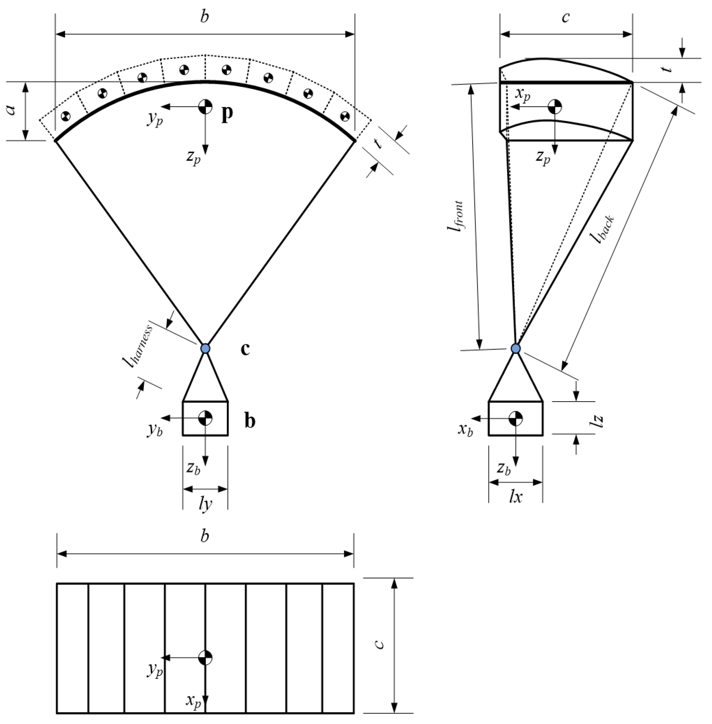
Figure 2.
Schematic diagram of parafoil pull-down.
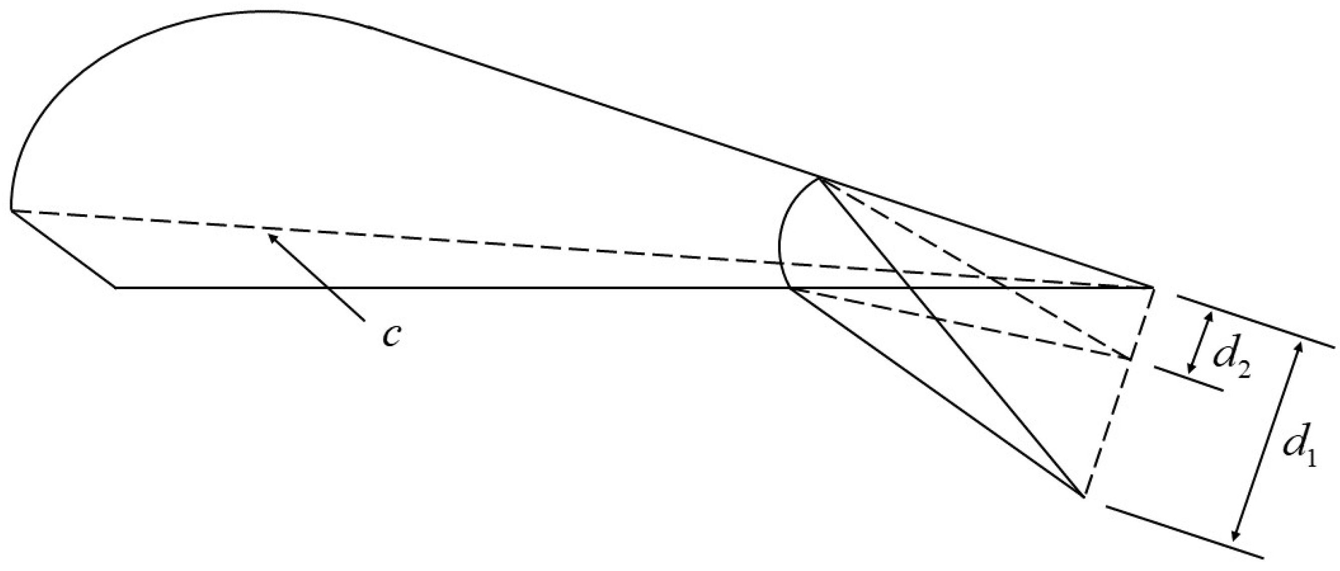
Figure 3.
Block diagram of tracking control method.

Figure 4.
Schematic diagram of curved terrains and cylindrical threat areas.
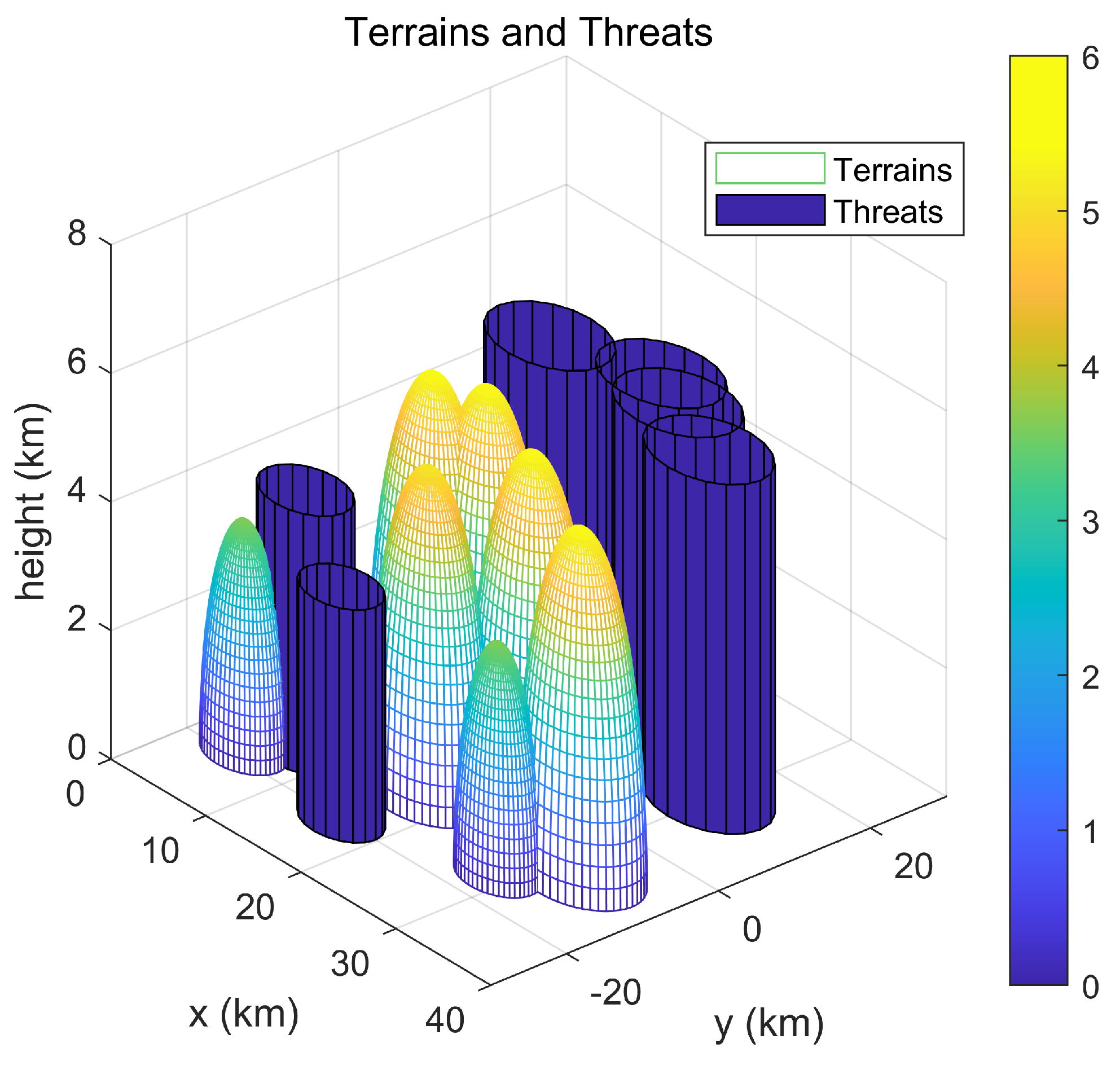
Figure 5.
Rotational wind field.

Figure 6.
Crosswind field.
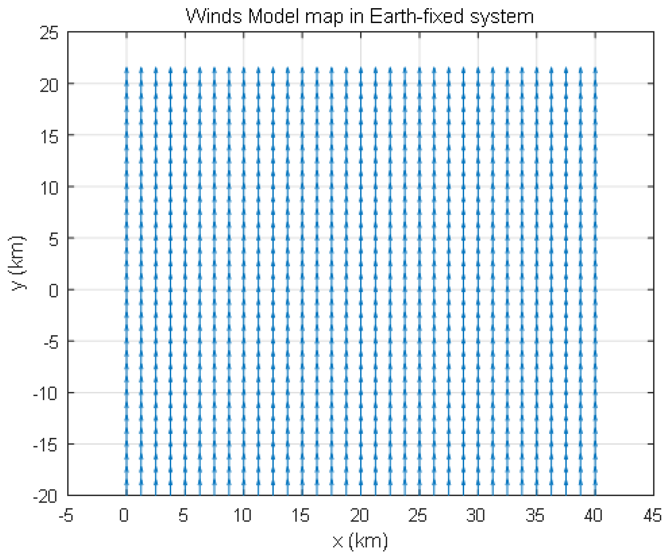
Figure 7.
Headwind field.
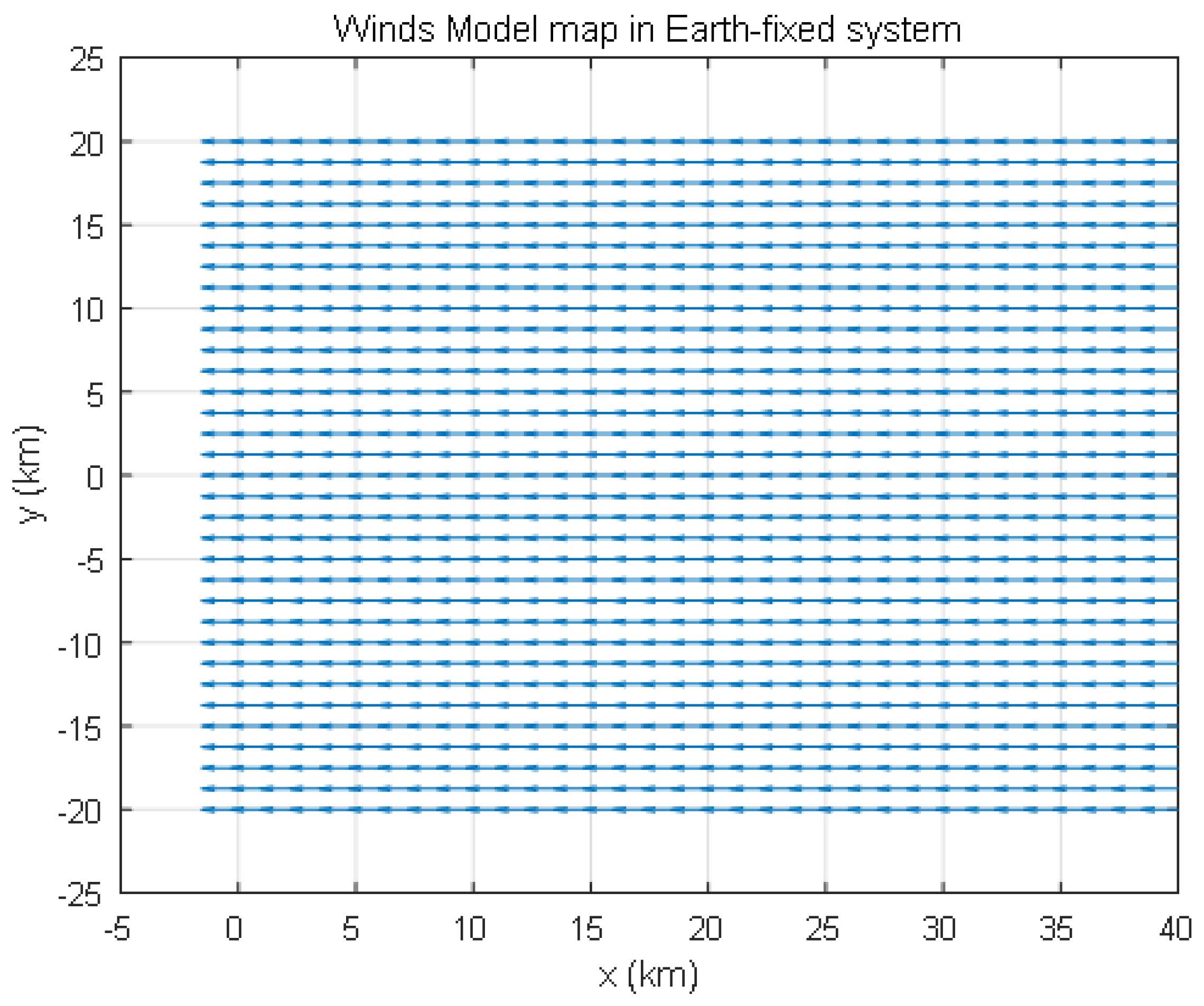
Figure 8.
Comparison of Parafoil Planned Paths under Different Planning Methods.
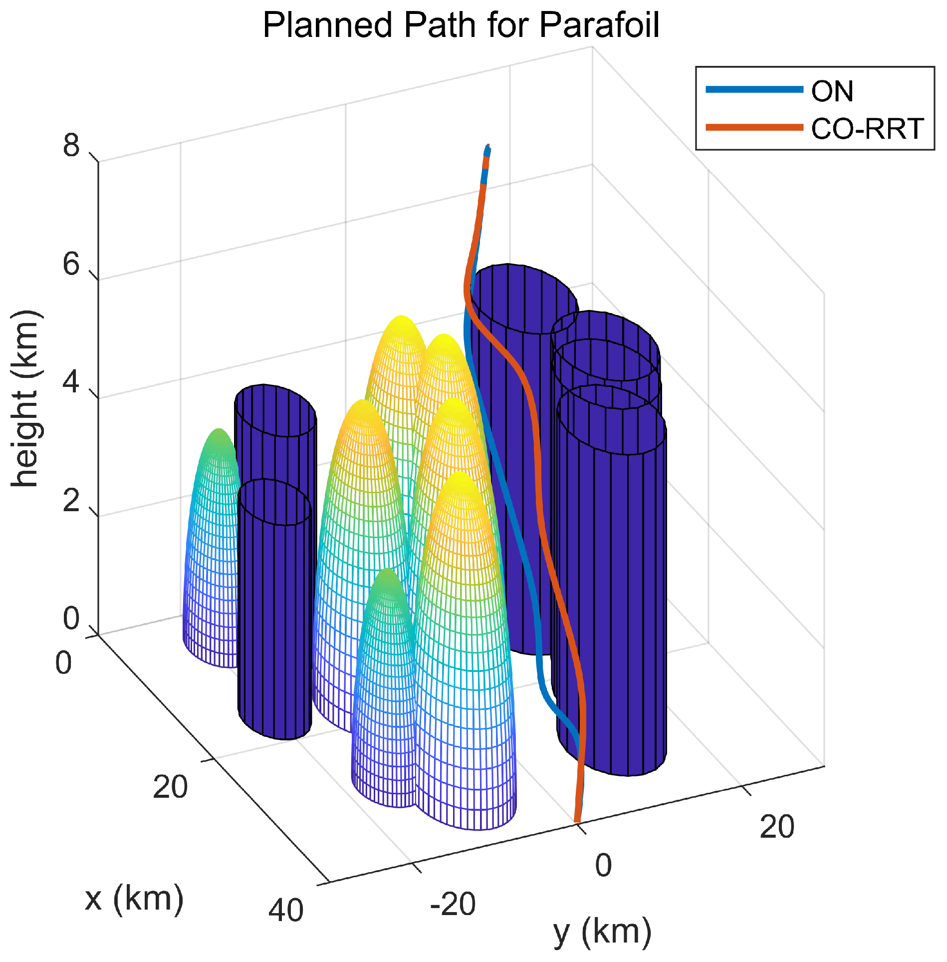
Figure 9.
Comparison of Parafoil Planned Velocities under Different Planning Methods.
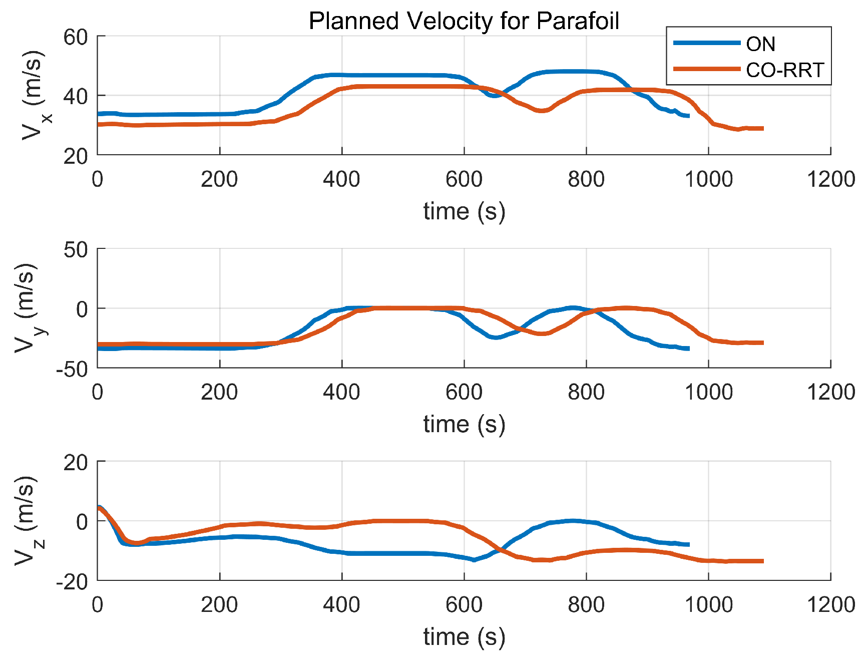
Figure 10.
Comparison of Parafoil Planned Accelerations under Different Planning Methods.
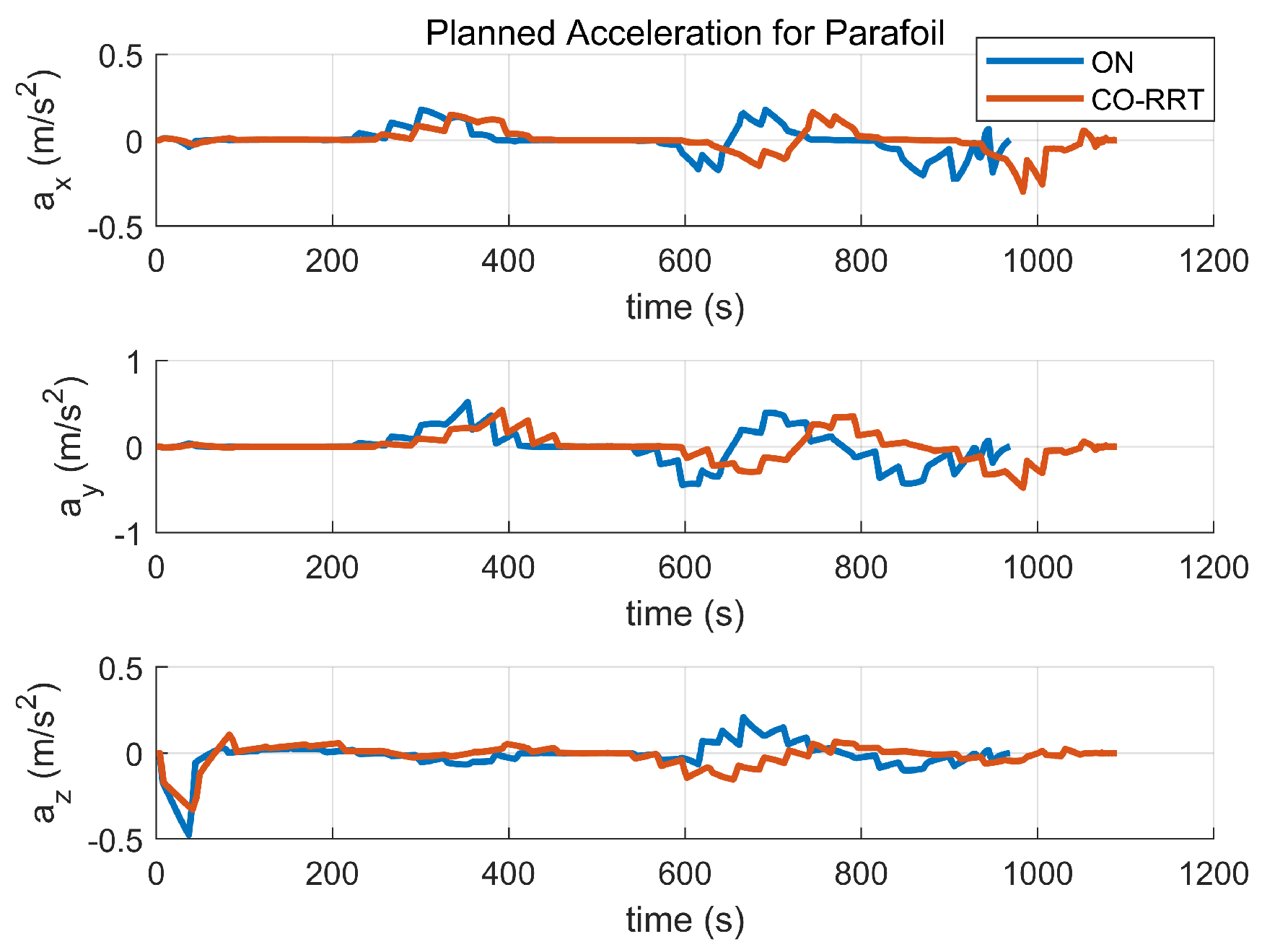
Figure 11.
Comparison of Parafoil Planned Paths under Different Wind Fields.
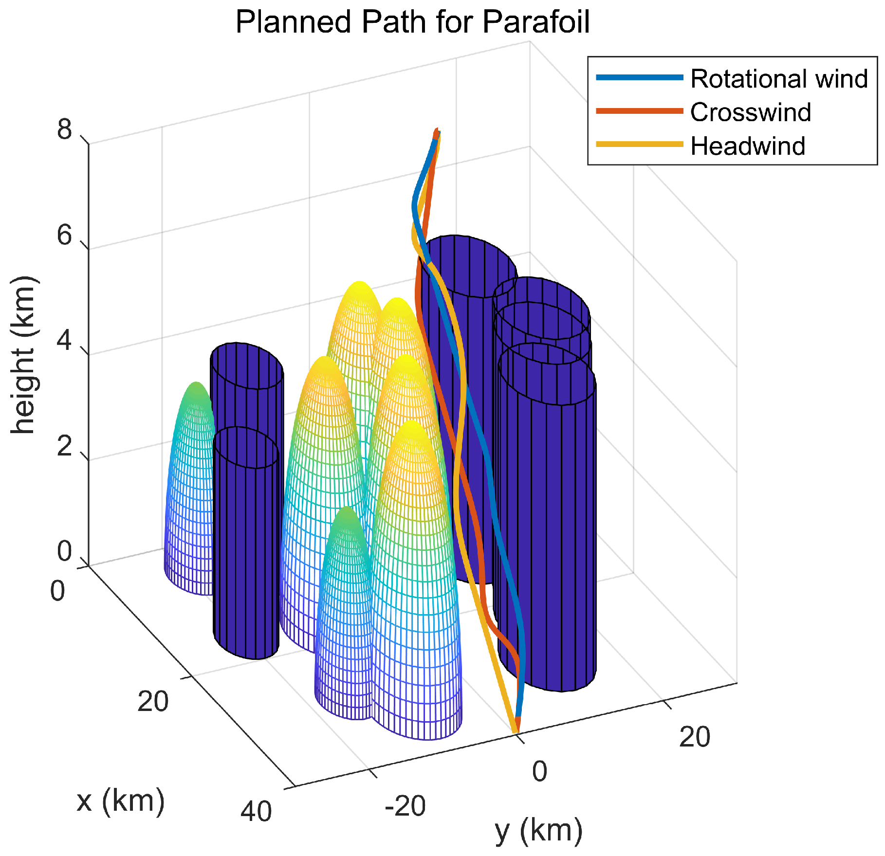
Figure 12.
Comparison of Parafoil Planned Velocities under Different Wind Fields.
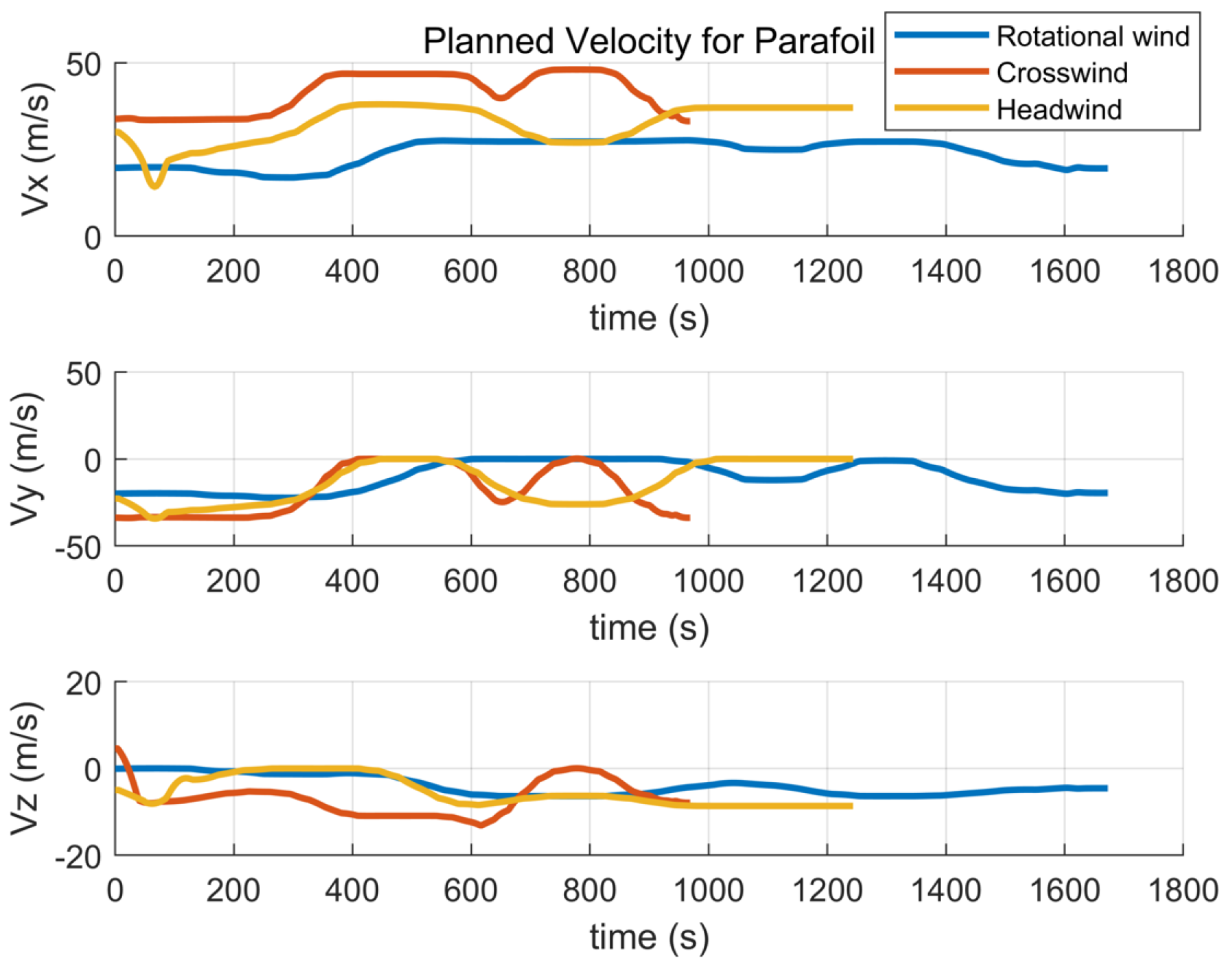
Figure 13.
Comparison of Parafoil Planned Accelerations under Different Wind Fields.
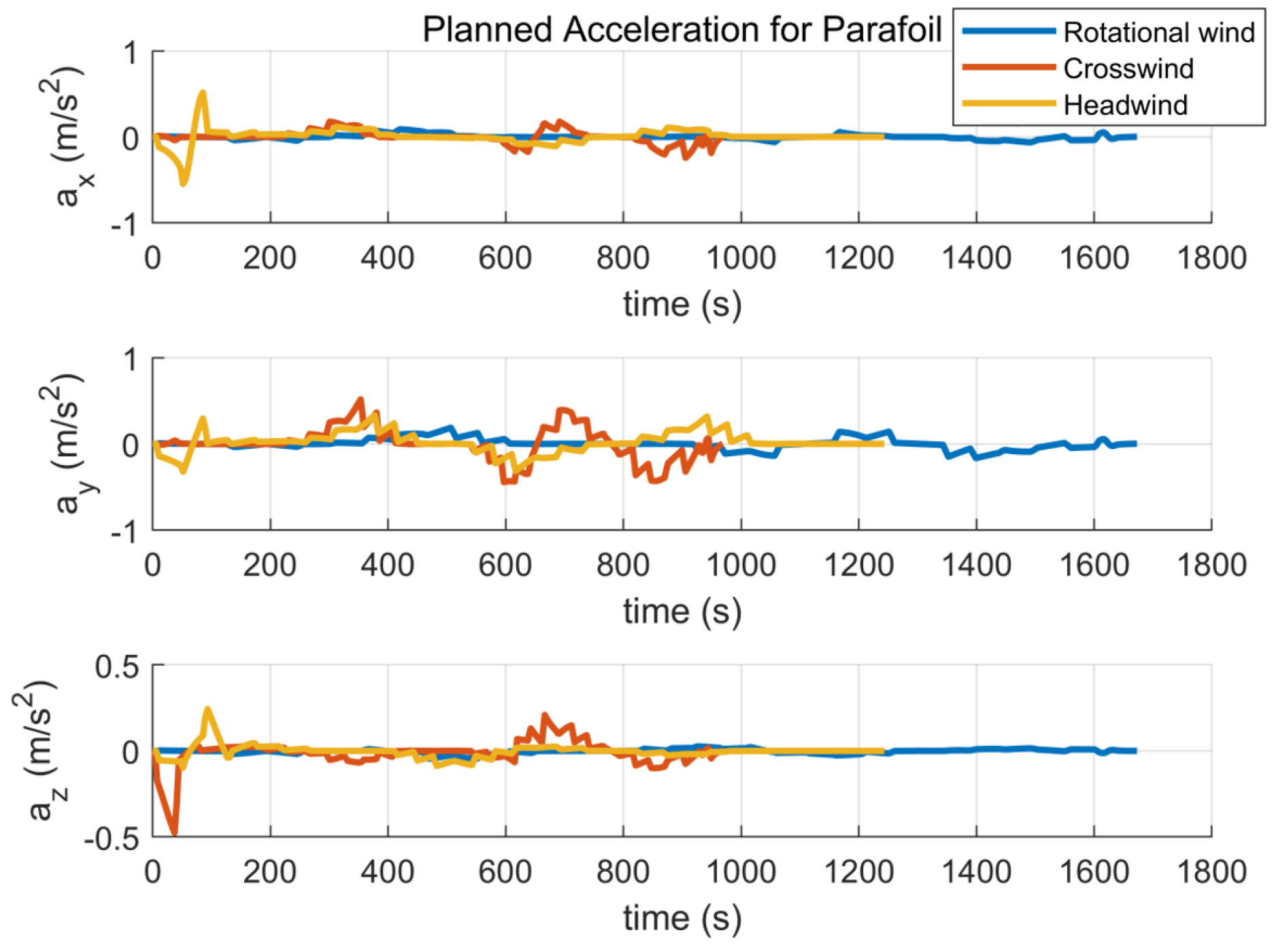
Figure 14.
Parafoil Tracked Path under Sliding Mode Control.
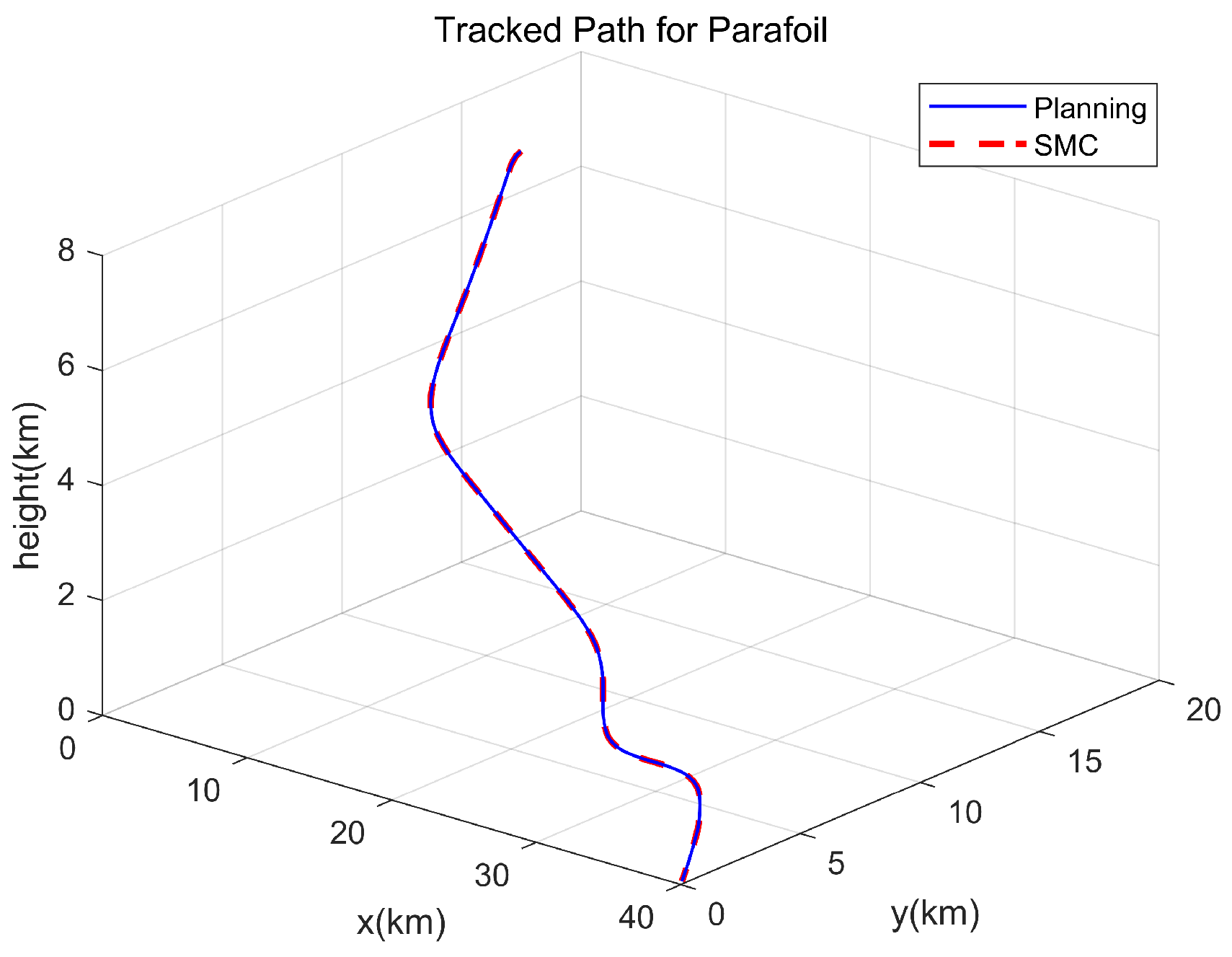
Figure 15.
Parafoil Tracked Path under ADRC–PID.
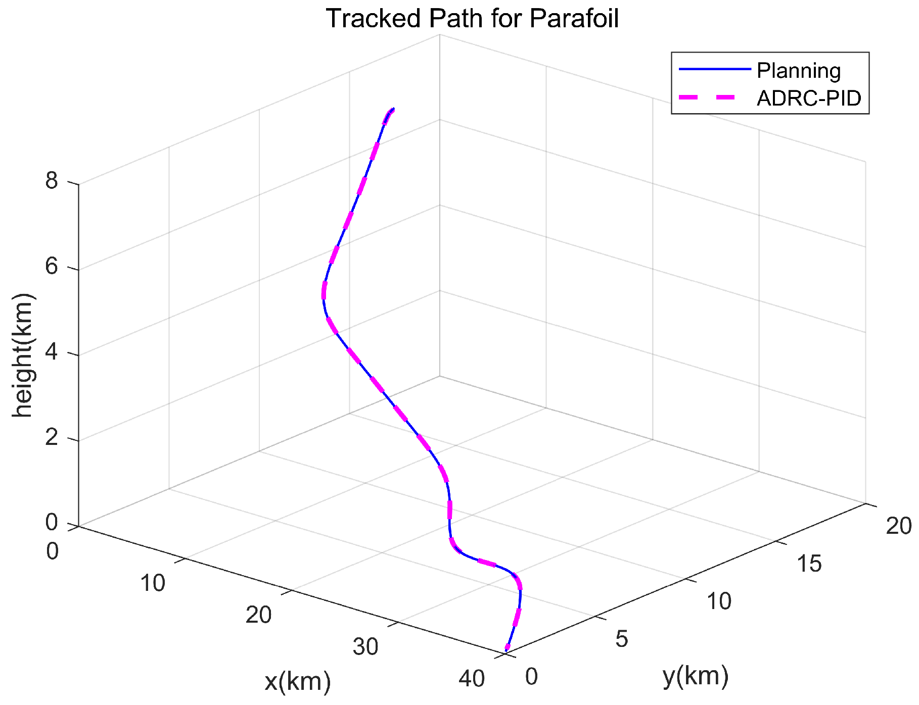
Figure 16.
Comparison of Parafoil Tracked Velocities under Different Tracking Methods.
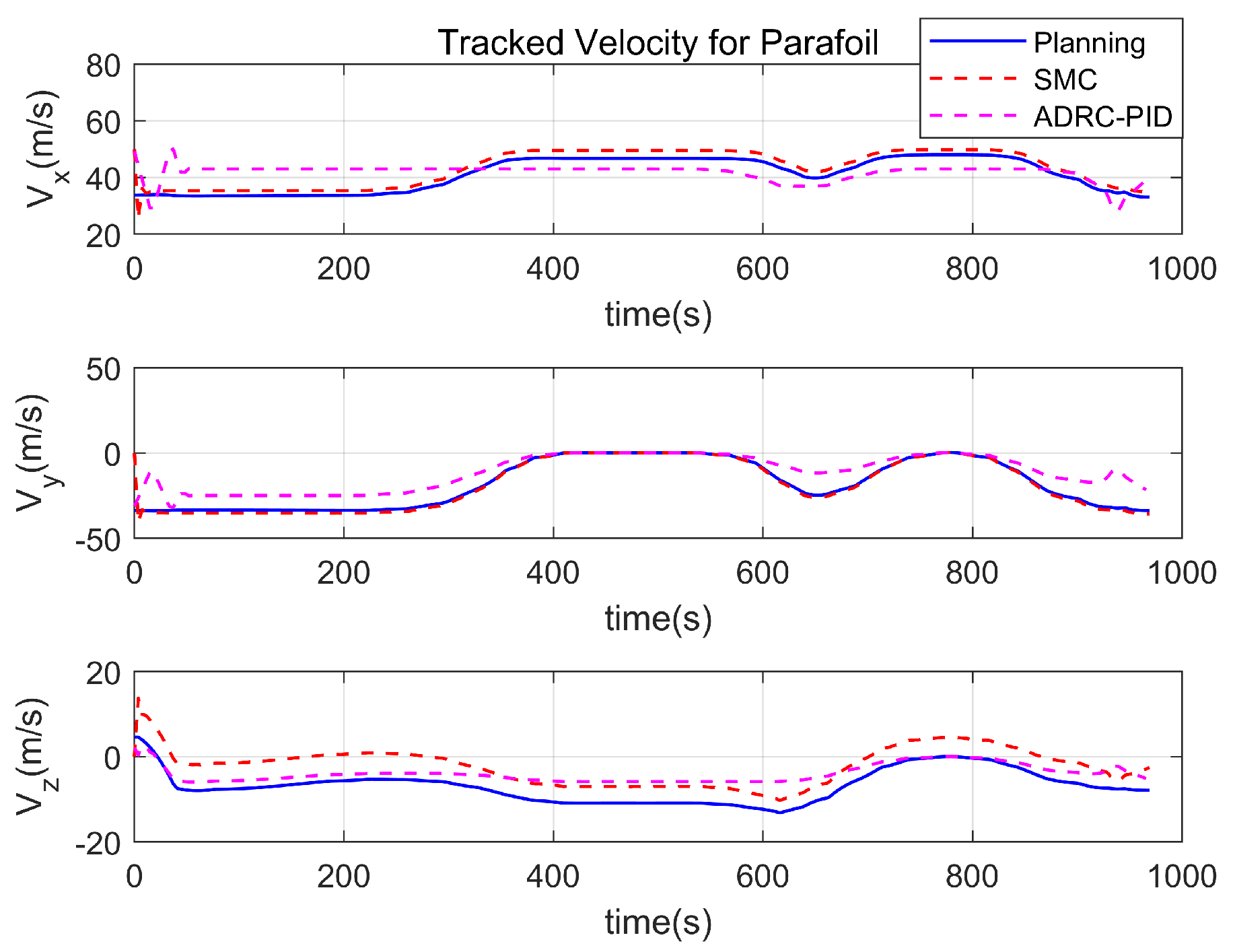
Figure 17.
Comparison of Parafoil Tracked Accelerations under Different Tracking Methods.
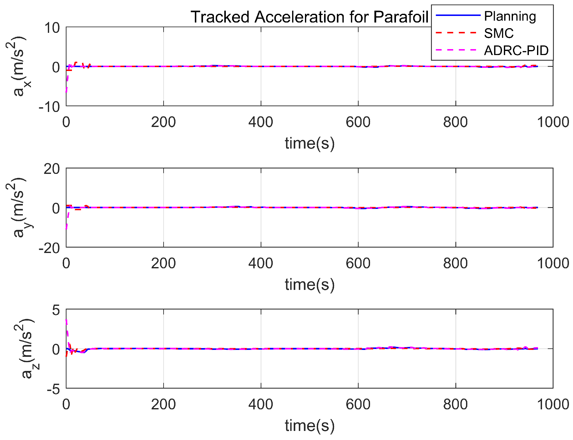
Figure 18.
Comparison of Parafoil Path Tracking Errors under Different Tracking Methods.
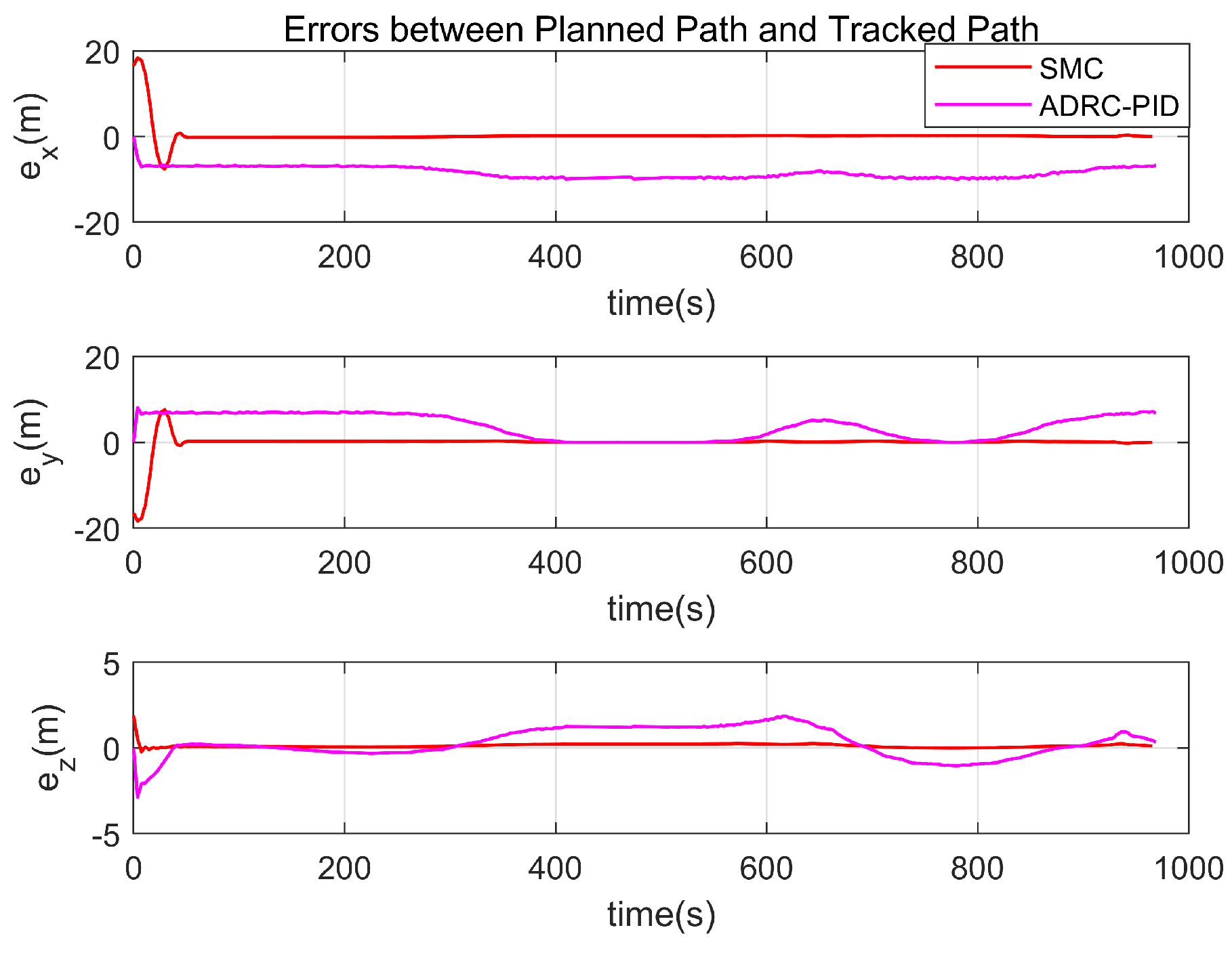
Figure 19.
Control Input of Parafoil Path Tracking.

Table 1.
Values of relevant aerodynamic coefficients.
| Coefficients | Values | Coefficients | Values |
|---|---|---|---|
| −0.0095 | 0.2350 | ||
| −0.0060 | 0.0957 | ||
| −0.0014 | 0.1368 | ||
| −0.1330 | 0.2940 | ||
| 0.0100 | −0.0063 | ||
| 0.0005 | 0.0155 | ||
| −0.0130 | −1.864 | ||
| −0.0350 |
Table 2.
Simulation Conditions for Parafoil Path Planning.
| Method | Wind Field | Starting Position/km | Landing Position/km |
|---|---|---|---|
| ON | Crosswind | [0, 17.5, 6.5] | [40, 0, 0] |
| CO–RRT | Crosswind | [0, 17.5, 6.5] | [40, 0, 0] |
| ON | Rotational wind | [0, 17.5, 6.5] | [40, 0, 0] |
| Crosswind | [0, 17.5, 6.5] | [40, 0, 0] | |
| Headwind | [0, 17.5, 6.5] | [40, 0, 0] |
Table 3.
Simulation Conditions for Parafoil Path tracking.
| Method | Wind Field | Starting Position/km | Landing Position/km |
|---|---|---|---|
| SMC | Crosswind | [0, 17.5, 6.5] | [40, 0, 0] |
| ARDC–PID | Crosswind | [0, 17.5, 6.5] | [40, 0, 0] |
Table 4.
Tracking Errors.
| Method | /m | /m | /m | /m | /m |
|---|---|---|---|---|---|
| SMC | 0.23 | 0.63 | 0.14 | 0.96 | 25.97 |
| ADRC–PID | 6.53 | 2.39 | 0.36 | 7.72 | 12.98 |
Disclaimer/Publisher’s Note: The statements, opinions and data contained in all publications are solely those of the individual author(s) and contributor(s) and not of MDPI and/or the editor(s). MDPI and/or the editor(s) disclaim responsibility for any injury to people or property resulting from any ideas, methods, instructions or products referred to in the content. |
© 2023 by the authors. Licensee MDPI, Basel, Switzerland. This article is an open access article distributed under the terms and conditions of the Creative Commons Attribution (CC BY) license (https://creativecommons.org/licenses/by/4.0/).
Share and Cite
MDPI and ACS Style
Li, Z.; Nan, Y. Optimal Path Planning and Tracking Control Methods for Parafoil. Appl. Sci. 2023, 13, 8115. https://doi.org/10.3390/app13148115
AMA Style
Li Z, Nan Y. Optimal Path Planning and Tracking Control Methods for Parafoil. Applied Sciences. 2023; 13(14):8115. https://doi.org/10.3390/app13148115
Chicago/Turabian StyleLi, Zhihan, and Ying Nan. 2023. "Optimal Path Planning and Tracking Control Methods for Parafoil" Applied Sciences 13, no. 14: 8115. https://doi.org/10.3390/app13148115
Note that from the first issue of 2016, this journal uses article numbers instead of page numbers. See further details here.