An Improved Lightweight Dense Pedestrian Detection Algorithm

Abstract

Due to the limited memory and computing resources in the real application of target detection, the method is challenging to implement on mobile and embedded devices. In order to achieve the balance between detection accuracy and speed in pedestrian-intensive scenes, an improved lightweight dense pedestrian detection algorithm GS-YOLOv5 (GhostNet GSConv- SIoU) is proposed in this paper. In the Backbone section, GhostNet is used to replace the original CSPDarknet53 network structure, reducing the number of parameters and computation. The CBL module is replaced with GSConv in the Head section, and the CSP module is replaced with VoV-GSCSP. The SloU loss function is used to replace the original IoU loss function to improve the prediction box overlap problem in dense scenes. The model parameters are reduced by 40% and the calculation amount is reduced by 64% without losing the average accuracy, and the detection accuracy is improved by 0.5%. The experimental results show that the GS-YOLOv5 can detect pedestrians more effectively under limited hardware conditions to cope with dense pedestrian scenes, and it is suitable for the online real-time detection of pedestrians.

1. Introduction

Pedestrian detection, as an important branch of target detection, has received a lot of attention from researchers due to its great potential in various engineering fields such as visual tracking [1], pedestrian re-identification [2], and behavior recognition [3]. Many target detection algorithms have emerged as a result of the quick development of deep learning. The need for lightweight models is particularly urgent because these algorithms place a focus on improving the accuracy, and they ignore issues with algorithmic model size and detection speed which largely determine how practical the algorithms are and whether they can be used on edge computing devices.

Deep-learning-based target detection algorithms can be broadly classified into two categories according to their algorithmic process characteristics: two-stage target detection algorithms and one-stage target detection algorithms. Two-stage target detection algorithms are mainly represented by the region-based convolutional neural networks (R-CNNs) [4,5,6] series, which have higher detection accuracy but slower detection speed. One-stage target detection algorithms are represented by the single-shot multi-box detector (SSD) [7] series and the You Only Look Once (YOLO) [8,9,10,11,12] series, which are reformulated as a regression problem that directly predicts image pixels as objects and their wraparound box properties [13]. These detection algorithms are of mediocre accuracy; however, they are rapid and frequently utilized in industry. YOLO is one of the quickest object detection algorithms available, several orders of magnitude faster than other target detection techniques. YOLO is a target detection technique that differs from region-based algorithms; the network outputs a class probability and an offset value for each bounding box. The bounding boxes with class probabilities greater than a certain threshold are chosen and utilized to locate targets in the image [14].

Most of the current pedestrian detection tasks are tested and run on high-performance graphics processing units (GPUs), which cannot handle a large number of convolutional computations due to the different computational power of embedded devices and high-performance GPUs. Therefore, a simplified version of the neural network is needed to meet the needs of embedded platforms [15]. Wang [16] pruned the YOLOv4-Tiny convolutional kernel in TRC-YOLO and implemented an extra convolutional layer in the network’s residual module to create a ResNet (CSPResNet) structure. Zhao [17] presented SAI-YOLO, a lightweight target detection network based on YOLOv4-Tiny with an InceptionV3 structure that replaces two CSPBlock modules with RES-SEBlock modules to lower the number of parameters and computational difficulties. In addition, to replace the original Leaky ReLU function, an enhanced ReLU (M-ReLU) activation function is developed. Guo [18] proposed the DBA module in LMSD-YOLO as a generic lightweight convolution unit to build the entire lightweight model; second, the improved S-MobileNet module is designed as the backbone feature extraction network, which can be used to enhance feature extraction without adding additional computation; then, the DSASFF module is proposed to achieve the adaptive fusion of multi-scale features with fewer parameters; and, finally, SIoU is used as a loss function to accelerate model convergence and improve detection accuracy. Zhang [19] suggested a portable target detection approach based on the MobileNetv2 and YOLOv4 algorithms. To decrease the number of model parameters and the size of the model, MobileNetv2 and depth-separable convolution are coupled. Due to the varying processing power of embedded devices and large servers, many edge computing devices and mobile terminals do not have the requisite computational capability for modern state-of-the-art networks in practical applications. The accuracy of pedestrian recognition is further reduced in pedestrian-dense environments due to several target frames overlapping each other. This research investigates a lightweight pedestrian detection model framework to fulfill real-time pedestrian identification in congested scenarios. In summary, some structural optimizations are made on the basis of the original YOLOv5 to make the model more suitable for the specificity of real-time detection. The contributions of this paper can be summarized as follows.

• Based on YOLOv5 to further reduce its number of parameters and computation, for the backbone feature extraction network part, GhostNet, a lightweight network, is used to replace the original CSPDarknet53, and, for the neck part, GSConv and VoV-GSCSP are used to replace it, reducing the space required for model storage, while significantly improving the detection speed in under-computing scenarios.
• For the problem of overlapping prediction frames in dense scenes, the original IoU loss function cannot solve the prediction frame screening task well when the targets are close together. We employ SIoU as the loss function in this paper, introduce the vector angle between the real frame and the prediction frame, and redefine the related loss function to increase the model’s accuracy in crowded scenarios.

2. Related Work

2.1. YOLO Object Detection Algorithm

Convolutional neural networks sprang to prominence in 2012, propelling the field of target detection to new heights. According to the computational processes, convolutional neural network (CNN)-based target detection algorithms can be split into one-stage and two-stage. Two-stage target detection methods have higher accuracy than one-stage, although one-stage target detection algorithms run faster. The first one-stage target detection technique is YOLOv1. The method divides the image into numerous grids, then predicts the location bounding box for each grid at the same time and gives the corresponding class probability. Despite running at 155 frames per second, YOLOv1 is slower than other methods like the two-stage approach and has a worse target recognition ability for small targets. The Visual Geometry Group (VGG)-16 of the original YOLOv1 is replaced by the DarkNet19 backbone feature extraction network in YOLOv2; for the classification task, YOLOv2 employs the target detection; and, to increase detection accuracy, speed, and the number of recognizable species for the classification task, YOLOv2 uses the joint training technique of target detection and classification along with Word Tree and other methods. However, YOLOv2 still cannot address the issue of YOLO’s poor detection accuracy for targets of various sizes and small targets. The greatest change in YOLOv3 is that it takes the concept of feature pyramid networks (FPNs) and employs three detection branches to detect objects of various sizes in order to increase detection accuracy. Based on the general structure of YOLOv3, YOLOv4 adds a number of techniques from the most recent deep-learning research, such as data augmentation, self-adversarial training, the introduction of an SSP module, etc., which significantly increases detection accuracy while maintaining the same running speed. The YOLOv5 algorithm, a target identification model that operates with high accuracy and high speed, was introduced by Glenn Jocher in 2020. YOLOv5 is built on a PyTorch implementation and works well on both embedded and mobile platforms. YOLOv5 also incorporates state-of-the-art computer vision; however, it is slightly less accurate than YOLOv4. YOLOv5 is offered in the x, l, m, and s models (from high to low precision and large to small model size), which provides a significant advantage in model deployment.

2.2. Model Lightweighting

If YOLO detection methods were to be installed on embedded devices, the YOLO network structure must be simplified. There are currently two methods for simplifying the YOLO network structure. One way is to use Nvidia’s TensorRT, which is accelerated for Nvidia GPUs so that the YOLO computation is optimized on the GPU of the embedded system. The other method is to use lightweight networks, which focus on lightweighting the network structure in terms of both model size and inference time while keeping as much accuracy as possible. Many lightweight networks have been proposed, such as MobileNet [20,21,22], ShuffleNet [23,24], GhostNet [25], etc. The core idea of MobileNet is to use a computation called a separable convolutional group. The name of the network indicates that it is mainly used for mobile devices [26]. The method of calculating convolution in the MobileNet network adopts the step of “separate–compute–merge”. By dividing the original 3 × 3 convolution into three 1 × 1 convolutions, the repeated computation of the convolution kernels is reduced. This reduces the computational effort and the number of parameters required [27]. ShuffleNet proposes channel-shuffling procedures to facilitate the sharing of information between channel groups. ShuffleNetv2 takes into account the target hardware’s actual speed for a simple model design. Although these models performed well with a little flop, the correlation and redundancy between feature maps were never fully utilized. Unlike the traditional convolutional operation used to generate redundant feature maps, GhostNet uses only a small amount of traditional convolution to generate part of the feature map, and then makes a simple linear change to this part of the feature map to obtain the required number of feature maps; this operation can increase the feature redundancy of maps. This method can increase redundancy of the feature map and “imitate” the impact of classical convolution. Given that TensorRT presently only supports Open Neural Network Exchange (ONNX), Caffe, and Universal Framework Format (UFF), which cannot be installed in most embedded systems, this study focuses on simplifying the network by adopting a lightweight network method.

3. Proposed Algorithm

3.1. Network Structure of GS-YOLOv5

Figure 1 depicts the model structure of the YOLOv5 [28] model, which is primarily composed of three parts. The Neck network mainly consists of feature pyramid networks (FPNs) and path aggregation networks (PANs), FPN conveys semantic information from the top down and PAN conveys location information from the bottom up. The Head part performs a prediction on the processed image features in three dimensions, generates bounding boxes, and predicts the class of the target.

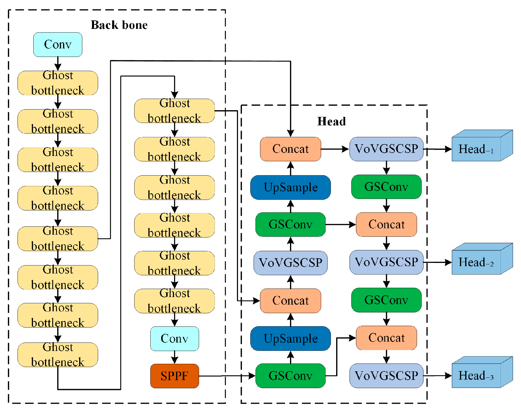
Figure 2 depicts the GS-YOLOv5 model structure. YOLOv5’s backbone network contains many convolution modules, batch normalization (BN) layers, etc., resulting in a huge model that requires a lot of flops and operations. Therefore, 14 Ghost bottleneck modules are used to greatly reduce the number of parameters and accelerate the training speed. The spatial pyramid pooling (SPP) module is replaced with spatial pyramid pooling fast (SPPF), which produces the same output as the SPP module but with improved computational efficiency. There are also a large number of common convolution and cross-stage partial network (CSP) structures in the neck of YOLOv5. To further construct a lightweight network, the convolutional block layer (CBL) module is replaced with GSConv (a new lightweight convolution method) in the Head section, and the CSP module is replaced with VoV-GSCSP (the one-shot aggregation method to design the cross-stage partial network). The whole algorithm is summarized in the pseudo-code in Algorithm 1.

Algorithm 1 Pseudocode of GS-YOLOv5

Input: Image I, confidence threshold T Output: Detected objects with their bounding boxes and labels Loading the pre-trained model M Scaling and normalizing the input image I Inputting the image I into the neural network to obtain the output feature map Using the feature map to predict each grid unit Predicting whether each grid unit contains an object Predicting the category of objects in each grid unit (using the softmax activation function) Predicting the location and size of objects in each grid unit (using the sigmoid activation function) Screening and removing the predicted bounding boxes Removing bounding boxes with a confidence lower than the threshold T Using a non-maximum suppression algorithm to remove overlapping bounding boxes Outputting the final prediction results, including the category, confidence, and location information of each object

3.1.1. GhostNet Optimized Backbone Section

The key to increasing the speed of YOLOv5 is to apply a lightweight network in the backbone portion of the network. The CSPDarknet53 is replaced with the GhostNet network, and the original CSPDarknet53 network structure is shown in Figure 3. The Focus module first splits the 640 × 640 × 3 image into a 320 × 320 × 12 feature map, and then performs a 3 × 3 convolution operation with an output channel of 32, resulting in a 320 × 320 × 32 feature map. The CBL module first conducts the convolution operation, followed by normalization and activation. CSP1_X divides the input into two branches. One branch goes through CBL, then X residual structures, then another convolution; the other branch is convolved directly, then the two branches are fused, go through the BN layer, then another activation, and finally go through CBL. The SPP module will use the maximum pooling of 5/9/13, respectively, and then performs concat fusion to improve the sensory field.

• Ghost Module

For image detection, YOLO employs multi-layer convolution, with 3 × 3 convolution accounting for the majority of the processing burden. GhostNet introduces a new Ghost Module that produces more features with fewer parameters. It is discovered that the feature maps generated by the mainstream deep neural network contain a huge number of similar feature maps, resulting in feature redundancy. To address this feature, the Ghost Module executes (cheap operations) simple linear operations on one of the feature maps, resulting in more comparable feature maps with fewer parameters, and similar feature maps are considered Ghosts of each other. The Ghost Module extracts the same features as conventional convolution by changing the superfluous features from the obtained feature maps using deep separable convolution. As illustrated in Figure 4, the Ghost Module first obtains the intrinsic map by using regular convolution, then executes a series of basic linear operations on each original feature, generates n Ghost feature maps, and then utilizes concat to obtain the final output. The linear operation is performed on each channel, and the amount of calculation is significantly less than that of conventional convolution.

B.

Ghost bottleneck

The Ghost bottleneck is intended for small CNNs that use the Ghost Module. As illustrated in Figure 5, the Ghost bottleneck is mostly composed of two stacked Ghost Modules. The first Ghost Module serves as an extension layer, allowing the number of channels to be increased. The second Ghost Module minimizes the number of channels that correspond to the shortcut path. We then connect shortcuts between the two Ghost Modules’ input and output.

The above-mentioned Ghost bottleneck is for stride = 1. In the case of stride = 2, the down-sampling layer implements the shortcut path, and a deep convolution of stride = 2 is placed between two Ghost Modules.

3.1.2. GSConv Optimization Neck Section

• Depth Separable Convolution (DSC) and Standard Convolution (SC)

The design of the lightweight network design could help to reduce the high computational cost. The main goal is to reduce the number of parameters and floating-point operations (FLOPs) by using deep separable convolution (DSC) operations, and the impact is noticeable. The disadvantage of DSC is also obvious: the channel information of the input image is separated during the calculation process; the ability resulted in feature extraction, and fusion is weaker than that of SC.

B.

GSConv

GhostNet makes use of the “halved” SC operation to retain channel interaction information. Nevertheless, the 1 × 1 dense convolution consumes more processing resources, and the results of utilizing “channel shuffle” has no effect on the SC results, and GhostNet returns to SC, which may affect a variety of factors. Many lightweight models use similar thinking to design the basic architecture, using only DSC from the beginning to the end of the deep neural network; however, the shortcomings of DSC are immediately magnified in the backbone, both for image categorization and detection. To ensure the DSC output is as near to SC as feasible, GSConv [29], a hybrid convolution of SC, DSC, and shuffle, is utilized. As shown in Figure 6, the information generated by SC (channel-dense convolution operation) is permeated to each part of the information generated by DSC using shuffle, which is a uniform mixing strategy. This method allows the information from the SC to be completely mixed into the output of the DSC, exchanging local feature information uniformly over different channels.

To speed up the prediction calculation, the feed image in the CNN almost has to go through a similar conversion procedure in the Backbone: spatial information is gradually delivered to the channel. And each space (width and height) compression and channel extension of the feature map will result in some semantic information being lost. Dense convolution amplifies the hidden connections between each channel, whereas sparse convolution eliminates these connections. GSConv protects these relationships as much as feasible while being time-efficient. The advantage of GSConv is particularly noticeable for lightweight detectors, owing to the improved nonlinear expression capabilities provided by the addition of the DSC layer and shuffle. However, if it is employed at all phases of the model, the network layer becomes deeper and the inference time increases dramatically. As a result, GSConv is only used in the Neck section.

C.

VoV-GSCSP

The Slim neck structure is used to minimize the computational complexity and inference time of the detector on the premise of assuring detector accuracy. GSConv completes the task of reducing computational complexity, but the task of reducing inference time while keeping accuracy necessitates the development of a new model.

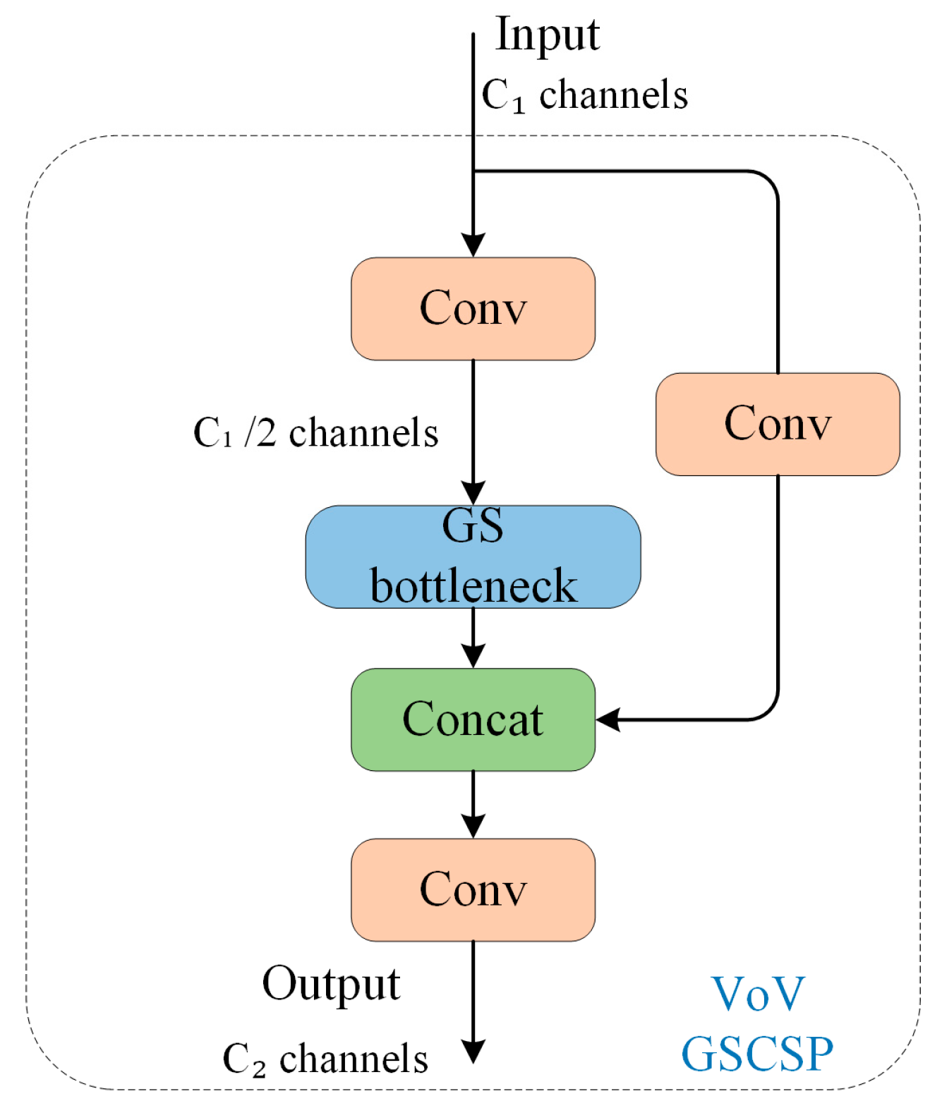
The GS bottleneck is built on the basis of GSConv. Figure 7 depicts the GS bottleneck module’s layout. Based on the theory of DensNet, VoVNet, and CSPNet, a cross-stage partial network (GSCSP) module VoV-GSCSP is designed by a one-time aggregation method. As illustrated in Figure 8, the structure is straightforward, the reasoning pace is quicker, and the hardware is more user-friendly.

3.2. SIoU Loss Function

3.2.1. Existing Loss Function Analysis

Although the design of depth models has been extensively researched, the loss function used for bounding box regression is also important in object detection [30]. The original IoU [31] loss can be expressed as the intersection ratio of the actual and predicted frames, as shown below:

$$\mathrm{I}\mathrm{o}\mathrm{U}=\frac{\mathrm{A}}{\mathrm{B}}, \mathrm{L}\mathrm{o}\mathrm{s}{\mathrm{s}}_{\mathrm{I}\mathrm{o}\mathrm{U}}=1-\mathrm{I}\mathrm{o}\mathrm{U}$$

(1)

where A is the intersection and B is the union. It does not differentiate between the cases where the two frames do not overlap. The GIoU [32] loss was then suggested using the following equation:

$$\mathrm{G}\mathrm{I}\mathrm{o}\mathrm{U}=\mathrm{I}\mathrm{o}\mathrm{U}-\frac{\mathrm{C}}{\mathrm{D}}, \mathrm{L}\mathrm{o}\mathrm{s}{\mathrm{s}}_{\mathrm{G}\mathrm{I}\mathrm{o}\mathrm{U}}=1-\mathrm{G}\mathrm{I}\mathrm{o}\mathrm{U}$$

(2)

where C is the difference set and D is the minimum circumscribed rectangle. When the prediction frame is inside the real frame and its area is equal, GIoU cannot identify the relative position relationship between the prediction frame and the real frame, which is why DIoU [33] introduces the center distance, which is defined as follows:

$$\mathrm{D}\mathrm{I}\mathrm{o}\mathrm{U}=\mathrm{I}\mathrm{o}\mathrm{U}-\frac{{\mathrm{d}}^2}{{\mathrm{c}}^2},\mathrm{L}\mathrm{o}\mathrm{s}{\mathrm{s}}_{\mathrm{D}\mathrm{I}\mathrm{o}\mathrm{U}}=1-\mathrm{D}\mathrm{I}\mathrm{o}\mathrm{U}$$

(3)

where d is the distance between the prediction center point of the frame and the real frame, and c is the diagonal distance of the minimum outer rectangle. The distance between the prediction frame and the real frame can be directly approximated by reducing the DIoU loss function, and the convergence speed is quick. DIoU cannot identify the relationship between the prediction frame and the real frame when the prediction frame is inside the real frame and the area of the prediction frame and the center distance are equal.

CIoU then adds the loss of detection frame scale to DIoU and raises the loss of length and breadth, resulting in a more consistent prediction frame with the real frame.

The following is the CIoU formula:

$$\mathrm{C}\mathrm{I}\mathrm{o}\mathrm{U}=\mathrm{I}\mathrm{o}\mathrm{U}-\frac{{\mathrm{d}}^2}{{\mathrm{c}}^2}-\frac{{\mathrm{v}}^2}{(1-\mathrm{I}\mathrm{o}\mathrm{U})+\mathrm{v}}, \mathrm{L}\mathrm{o}\mathrm{s}{\mathrm{s}}_{\mathrm{C}\mathrm{I}\mathrm{o}\mathrm{U}}=1-\mathrm{C}\mathrm{I}\mathrm{o}\mathrm{U}$$

(4)

where d is the distance between the predicted box’s center point and the real box, c is the diagonal distance of the smallest outside rectangle, and $\mathrm{v}$ is the aspect ratio’s similarity factor, defined as follows:

$$\mathrm{v}=\frac{4}{{\mathsf{\pi }}^2}{(\arctan \frac{{\mathrm{W}}_{\mathrm{b}}}{{\mathrm{H}}_{\mathrm{b}}}-\arctan \frac{{\mathrm{W}}_{\mathrm{p}}}{{\mathrm{H}}_{\mathrm{p}}})}^2$$

(5)

where ${\mathrm{W}}_{\mathrm{b}}$, ${\mathrm{H}}_{\mathrm{b}}$, ${\mathrm{W}}_{\mathrm{p}}$, and ${\mathrm{H}}_{\mathrm{p}}$ are the true frame width and height, as well as the predicted frame width and height, respectively.

3.2.2. SIoU Loss

The preceding loss function ignores the direction between the real and anticipated frames, resulting in a slow convergence rate. SIoU introduces the vector angle between the real and predicted frames and redefines the related loss function, which consists of four parts: angle cost, distance cost, shape cost, and IoU loss.

• Angle loss, defined as follows:

  $$\mathsf{\Lambda }=1-2\times {\sin }^2(\arcsin (\frac{{\mathrm{c}}_{\mathrm{h}}}{\mathsf{\sigma }})-\frac{\mathsf{\pi }}{4})$$

  (6)

  $$\mathsf{\sigma }=\sqrt{{({\mathrm{b}}_{{\mathrm{c}}_{\mathrm{x}}}^{\mathrm{g}\mathrm{t}}-{\mathrm{b}}_{{\mathrm{c}}_{\mathrm{x}}})}^2+{({\mathrm{b}}_{{\mathrm{c}}_{\mathrm{y}}}^{\mathrm{g}\mathrm{t}}-{\mathrm{b}}_{{\mathrm{c}}_{\mathrm{y}}})}^2}$$

  (7)

  $${\mathrm{c}}_{\mathrm{h}}=\max ({\mathrm{b}}_{{\mathrm{c}}_{\mathrm{y}}}^{\mathrm{g}\mathrm{t}},{\mathrm{b}}_{{\mathrm{c}}_{\mathrm{y}}})-\min ({\mathrm{b}}_{{\mathrm{c}}_{\mathrm{y}}}^{\mathrm{g}\mathrm{t}},{\mathrm{b}}_{{\mathrm{c}}_{\mathrm{y}}})$$

  (8)

  where ${\mathrm{c}}_{\mathrm{h}}$ is the height difference between the actual frame’s center point and the predicted frame’s center point, and $\mathsf{\sigma }$ is the distance between the real frame’s center point and the predicted frame’s center point. ${\mathrm{b}}_{{\mathrm{c}}_{\mathrm{x}}}^{\mathrm{g}\mathrm{t}},{\mathrm{b}}_{{\mathrm{c}}_{\mathrm{y}}}^{\mathrm{g}\mathrm{t}}$ are the coordinates of the center of the real frame, and ${\mathrm{b}}_{{\mathrm{c}}_{\mathrm{x}}},{\mathrm{b}}_{{\mathrm{c}}_{\mathrm{y}}}$ are the coordinates of the center of the predicted frame.
• Distance loss, defined as follows:

  $$\mathsf{\Delta }=2-{\mathrm{e}}^{-\mathsf{\gamma }{\mathsf{\rho }}_{\mathrm{x}}}-{\mathrm{e}}^{-\mathsf{\gamma }{\mathsf{\rho }}_{\mathrm{y}}}$$

  (9)

  $${\mathsf{\rho }}_{\mathrm{x}}={(\frac{{\mathrm{b}}_{{\mathrm{c}}_{\mathrm{x}}}^{\mathrm{g}\mathrm{t}}-{\mathrm{b}}_{{\mathrm{c}}_{\mathrm{x}}}}{{\mathrm{c}}_{\mathrm{w}}})}^2,{\mathsf{\rho }}_{\mathrm{y}}={(\frac{{\mathrm{b}}_{{\mathrm{c}}_{\mathrm{y}}}^{\mathrm{g}\mathrm{t}}-{\mathrm{b}}_{{\mathrm{c}}_{\mathrm{y}}}}{{\mathrm{c}}_{\mathrm{h}}})}^2,\mathsf{\gamma }=2-\mathsf{\Lambda }$$

  (10)

  ${\mathrm{c}}_{\mathrm{w}},{\mathrm{c}}_{\mathrm{h}}$ are the width and height of the minimum outer rectangle of the real box and the predicted box.
• Shape loss, defined as follows:

  $$\mathsf{\Omega }={(1-{\mathrm{e}}^{-{\mathsf{\omega }}_{\mathrm{w}}})}^{\mathsf{\theta }}+{(1-{\mathrm{e}}^{-{\mathsf{\omega }}_{\mathrm{h}}})}^{\mathsf{\theta }}$$

  (11)

  $${\mathsf{\omega }}_{\mathrm{w}}=\frac{\left|\mathrm{w}-{\mathrm{w}}^{\mathrm{g}\mathrm{t}}\right|}{\max (\mathrm{w},{\mathrm{w}}^{\mathrm{g}\mathrm{t}})},{\mathsf{\omega }}_{\mathrm{h}}=\frac{\left|\mathrm{h}-{\mathrm{h}}^{\mathrm{g}\mathrm{t}}\right|}{\max (\mathrm{h},{\mathrm{h}}^{\mathrm{g}\mathrm{t}})}$$

  (12)

  $\mathrm{w},\mathrm{h},{\mathrm{w}}^{\mathrm{g}\mathrm{t}},{\mathrm{h}}^{\mathrm{g}\mathrm{t}}$ are the width and height of the predicted and real frames, respectively, and $\mathsf{\theta }$ controls the degree of attention to shape loss.
• The SIoU loss function is defined as follows:

  $$\mathrm{L}\mathrm{o}\mathrm{s}{\mathrm{s}}_{\mathrm{S}\mathrm{I}\mathrm{o}\mathrm{U}}=1-\mathrm{I}\mathrm{o}\mathrm{U}+\frac{\mathsf{\Delta }+\mathsf{\Omega }}{2}$$

  (13)

4. Experiments

4.1. Experimental Environment and Parameter Description

The GS-YOLOv5 algorithm proposed in this paper for pedestrian detection is performed on Win10 OS with 11th Gen Intel^® Core™ i7-11700F 2.5 GHz with 8 total cores and 16 threads, and running at 2.5 GHz main frequency. The platform is paired with 2 × 3200 MHz 8 G memory sticks and Cuda uses version 11.7.102 and cudnn uses version 8.4. The deep-learning framework uses Pytorch version 1.7.1, and the experimental language is Python 3.8.

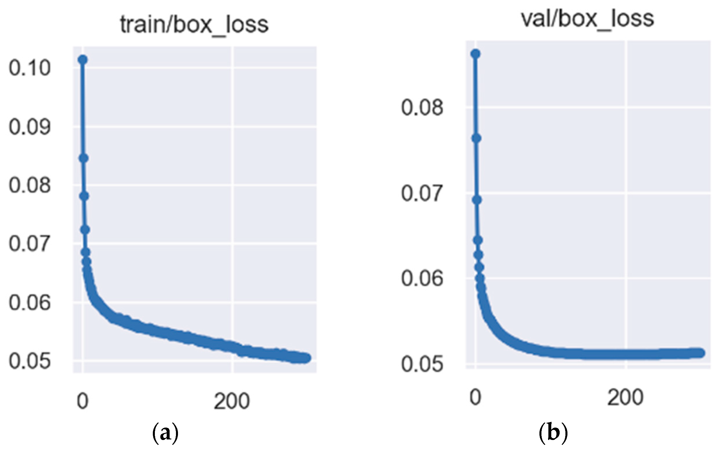
Before the model training, the initial learning rate is set to 0.01, the decay coefficient of weights is set to $5\times {10}^{-4}$, the batch size is set to 8, the size of the input image is uniformly adjusted to 640 × 640, and the Mosica and Mixup data enhancement strategies are used. The cosine annealing algorithm adjusts the learning rate, the cosine annealing hyperparameter is set to 0.1, and the model is trained 300 times. The loss value for each epoch was recorded, and Figure 9 depicts the loss convergence curve of the GS-YOLOv5.

The loss convergence curves illustrate that the training and validation losses continue to reduce and eventually converge to the minimum value. The GS-YOLOv5 model is free of divergence and overfitting issues, confirming its usefulness.

In the worst case, the running time of the GS-YOLOv5 algorithm can be represented by a Big O symbol. Specifically, the running time in the worst case can be expressed as the $\mathrm{O}({\mathrm{N}}^2\times \mathrm{M})$, where N is the size of the input image (the number of pixels) and M is the number of bounding boxes. In the worst case, the GS-YOLOv5 algorithm requires feature extraction, decoding, and prediction of each bounding box, which involves the processing and calculation of the feature map. Therefore, the running time of the algorithm is quadratically related to the size of the input image and the number of bounding boxes.

4.2. Datasets

With the availability of existing benchmark datasets, significant progress has been made in pedestrian detection. Yet, there is a diversity and density mismatch between current pedestrian detection benchmarks and actual needs. Most existing datasets, in particular, are derived from vehicles crossing regular traffic scenes, which usually results in insufficient diversity; additionally, highly obscured crowd scenes still lack representation, resulting in low density. In this paper, WiderPerson, a large and diverse dataset, was used as the training set for the GS-YOLOv5 detection model, which includes five types of annotations for a variety of scenes and is no longer limited to traffic scenes. There are 13,382 photos and 399,786 annotations in total, which indicates that each image includes roughly 30 annotations, indicating that the collection comprises dense pedestrians with varying occlusions. As a result of the large changes in context and occlusion, pedestrians in the WiderPerson dataset are exceedingly difficult and suited for pedestrian recognition model training in outdoor scenarios.

The performance of this paper’s pedestrian detection algorithm is verified in complex pedestrian occlusion situations using the CrowdHuman dataset, which was released by Kuang-Shi for pedestrian detection, with the majority of the image data coming from Google searches. With 15,000 images in the training set, 5000 images in the test set, and 4370 images in the validation set, the dataset is reasonably large. The training and validation sets contain a total of 470 K instances, with roughly 23 humans per image and a variety of occlusions. Each human instance has a bounding box for the head, a bounding box for the visible region, and a bounding box for the entire body.

4.3. Evaluation Metrics

Three evaluation metrics were used in this experiment to evaluate the performance of the algorithm.

Precision is the percentage of samples predicted to be positive that are actually positive. The formula is as follows:

$$\mathrm{Pr}\mathrm{e}\mathrm{c}\mathrm{i}\mathrm{s}\mathrm{i}\mathrm{o}\mathrm{n}(\mathrm{c}\mathrm{l}\mathrm{a}\mathrm{s}\mathrm{s}\mathrm{e}\mathrm{s})=\frac{\mathrm{T}\mathrm{P}}{\mathrm{T}\mathrm{P}+\mathrm{F}\mathrm{P}}$$

(14)

where TP indicates that positive samples are predicted to be positive and FP indicates that negative samples are predicted to be positive.

Recall is the percentage of all positive samples that are actually predicted to be positive. The formula is as follows:

$$\mathrm{Re}\mathrm{c}\mathrm{a}\mathrm{l}\mathrm{l}(\mathrm{c}\mathrm{l}\mathrm{a}\mathrm{s}\mathrm{s}\mathrm{e}\mathrm{s})=\frac{\mathrm{T}\mathrm{P}}{\mathrm{T}\mathrm{P}+\mathrm{F}\mathrm{N}}$$

(15)

where FN indicates that a positive sample is predicted to be a negative sample.

mAP is the average category AP, which is the AP of all categories divided by the total number of categories. The formula is as follows:

$$\mathrm{m}\mathrm{A}\mathrm{P}=\frac{{\displaystyle \sum \mathrm{A}\mathrm{P}}}{\mathrm{N}(\mathrm{C}\mathrm{l}\mathrm{a}\mathrm{s}\mathrm{s}\mathrm{e}\mathrm{s})}$$

(16)

where AP is the average correct rate, which represents the result of good or bad detection for each class: the area of the interpolated precision–recall curve with the X-axis envelope. The formula is as follows:

$$\mathrm{A}\mathrm{P}={\displaystyle \sum _{\mathrm{i}=1}^{\mathrm{n}-1}({\mathrm{r}}_{\mathrm{i}+1}-{\mathrm{r}}_{\mathrm{i}})}{\mathrm{P}}_{\mathrm{int}\mathrm{e}\mathrm{r}}({\mathrm{r}}_{\mathrm{i}}+1)$$

(17)

where ${\mathrm{r}}_1,{\mathrm{r}}_2,\dots ,{\mathrm{r}}_{\mathrm{n}}$ are the recall values corresponding to the first interpolation of the precision interpolation segment in ascending order.

mAP0.5 means that the value of IoU is taken as 50%. mAP0.5:0.95 means that the value of IoU is taken from 50% to 95% in steps of 5%, and then the mean value of mAP under these IoU is calculated.

4.4. Experimental Results

4.4.1. Ablation Experiments

As shown in

Table 1. Comparison of model performance.

	GhostNet	GSConv	SIoU	mAP0.5:0.95	Param	FLOPs
Model 1				0.316	21.04 M	47.9 G
Model 2	√			0.319	12.12 M	20.0 G
Model 3	√	√		0.318	12.55 M	17.3 G
Model 4	√	√	√	0.321	12.55 M	17.3 G

, where “√” indicates the corresponding method in each model, it can be seen that the parameters of the improved Model 2 are reduced by about 42% compared to the original model. Meanwhile, the mAP value of Model 2 is slightly improved compared to Model 1. The results show that the backbone structure of GhostNet exhibits good lightweight performance without sacrificing detection accuracy. In terms of detection speed, the FLOPs are 47.9 G for Model 1, 20.0 G for Model 2, and 17.3 G for Model 3. Compared with Model 1 without the lightweight structure, Model 2 optimized with GhostNet improved 58% in terms of computation and Model 3 with GhostNet and GSConv improved 64%, indicating a further reduction in the computation of the model with the addition of GSConv. In summary, the application of the lightweight structure is indeed beneficial for reducing the number of parameters and improving the detection speed.

Compared with Model 3, the mAP value of Model 4 improved by 0.3%, but the number of parameters and computation did not increase, indicating the effectiveness of SIoU in improving detection performance. The mAP value of Model 4 was improved by 0.5% compared to Model 1. In summary, SIoU does improve the detection accuracy of the model without increasing the computational cost.

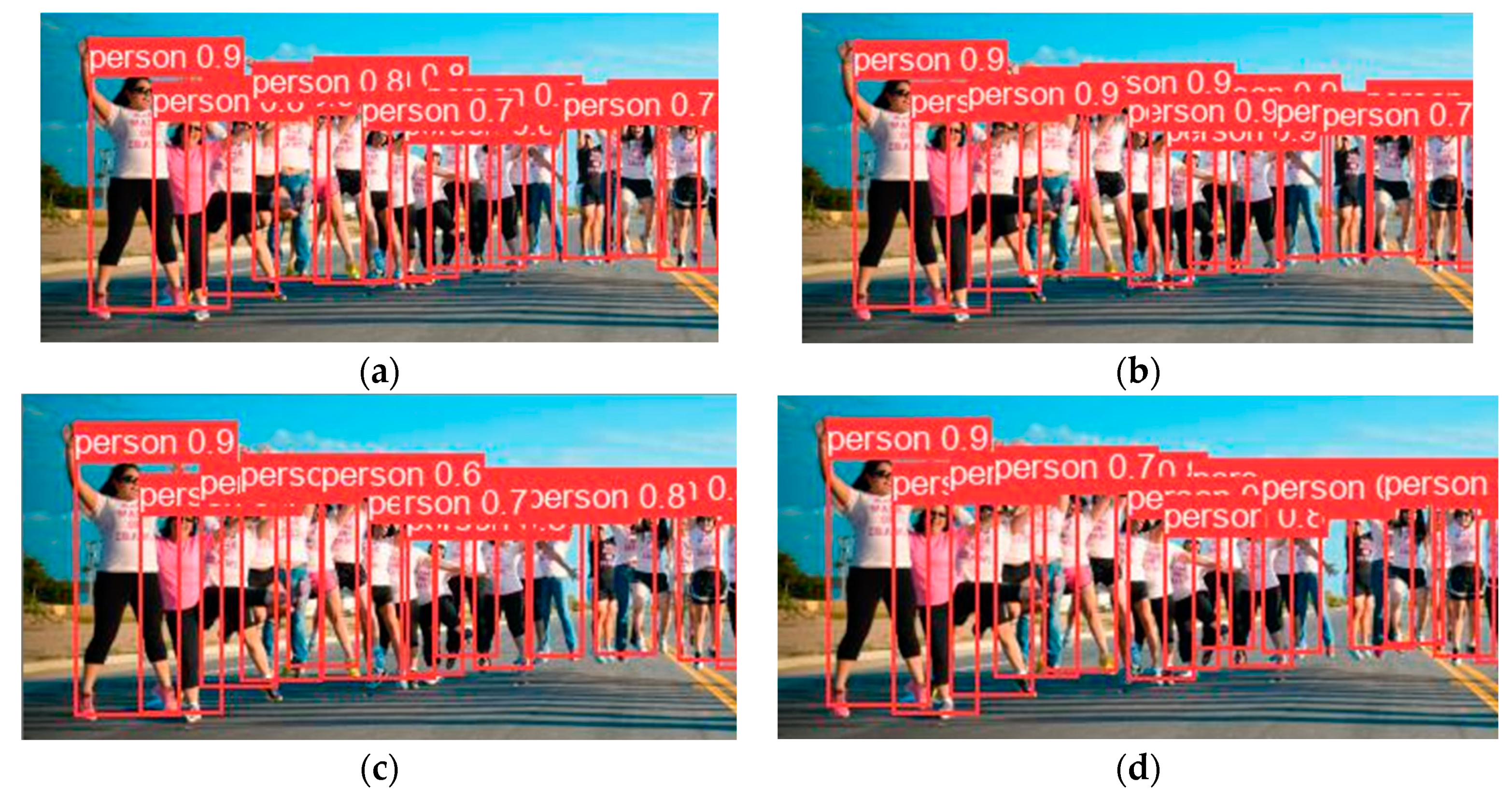
Models 1, 2, 3, and 4 were tested on the CrowdHuman dataset, and Figure 10 shows an example of image prediction for the above models.

From the above comparison results, it can be seen that Model 4 has no degradation in detection accuracy compared with other models, achieving a reduction in the number of parameters and computation of the network without a loss of accuracy.

Table 2. Test results on the CrowdHuman dataset.

Models	mAP0.5	mAP0.5:0.95	p	R
Model 1	0.601	0.316	0.779	0.38
Model 2	0.597	0.319	0.834	0.33
Model 3	0.598	0.318	0.85	0.319
Model 4	0.599	0.321	0.854	0.317

shows the test results of the GS-YOLOv5 on the CrowdHuman dataset. There is an improvement in mAP and precision for Model 4 compared to Model 1, Model 2, and Model 3.

4.4.2. Comparison of Detection Performance with Other Algorithm

In order to further verify the effectiveness of the algorithm in this paper, the GS-YOLOv5 algorithm was compared with other improved algorithms. The comparison results are shown in

Table 3. Comparison results of other algorithms on the CrowdHuman dataset.

Models	mAP0.5	mAP0.5:0.95	p	R
YOLOv5 + GhostNet + GSConv + SIoU	0.599	0.321	0.854	0.317
YOLOv5 + MobileNetV3	0.473	0.185	0.668	0.408
YOLOv5 + ShuffleNetV2	0.473	0.186	0.654	0.414
YOLOv5 + EfficientLite	0.505	0.204	0.689	0.437

.

As can be seen from Table 3, the GS-YOLOv5 algorithm proposed in this paper has a great improvement in mAP and precision, indicating that the GS-YOLOv5 satisfies the balance between detection accuracy and speed and is suitable for real-time pedestrian detection in dense scenes.

5. Conclusions

An improved YOLOv5 lightweight dense pedestrian detection algorithm is proposed in this article. The algorithm’s running speed is improved to solve the problem of real-time detection of dense pedestrians under the premise of keeping a certain accuracy and robustness in pedestrian-dense scenes. For picture feature extraction and feature fusion, it employs a lightweight backbone network and neck. Furthermore, in dense scenes, the SIoU loss function is used to improve the prediction box overlap issue. The experimental results on the CrowdHuman dataset show that the GS-YOLOv5 model’s number of parameters is reduced by 40% compared to the original YOLOv5, and the amount of calculation is reduced by 64%, significantly improving the detector’s detection speed. The mAP value is raised by 0.3% after SIoU is added without increasing the computational cost. The limitation of this method is that when real-time pedestrian detection meets the requirements, the calculation accuracy is not significantly improved. Shortly, more advanced algorithms for dense pedestrian detection can be researched further to enhance the algorithm’s overall performance and efficiency.

References

1. Lan, X.; Zhang, S.; Yuen, P.C. Robust Joint Discriminative Feature Learning for Visual Tracking. In Proceedings of the Twenty-Fifth International Joint Conference on Artificial Intelligence (IJCAI-16), New York, NY, USA, 9–15 July 2016; pp. 3403–3410. [Google Scholar]
2. Ma, A.J.; Li, J.; Yuen, P.C.; Li, P. Cross-domain person reidentification using domain adaptation ranking svms. IEEE Trans. Image Process. 2015, 24, 1599–1613. [Google Scholar] [CrossRef] [PubMed]
3. Ma, A.J.; Yuen, P.C.; Zou, W.W.; Lai, J.H. Supervised spatio-temporal neighborhood topology learning for action recognition. IEEE Trans. Circuits Syst. Video Technol. 2013, 23, 1447–1460. [Google Scholar] [CrossRef]
4. Girshick, R.; Donahue, J.; Darrell, T.; Malik, J. Rich feature hierarchies for accurate object detection and semantic segmentation. In Proceedings of the IEEE Conference on Computer Vision and Pattern Recognition, Columbus, OH, USA, 23–28 June 2014; pp. 580–587. [Google Scholar]
5. Girshick, R. Fast r-cnn. In Proceedings of the IEEE International Conference on Computer Vision, Santiago, Chile, 7–13 December 2015; pp. 1440–1448. [Google Scholar]
6. Ren, S.; He, K.; Girshick, R.; Sun, J. Faster R-CNN: Towards Real-Time Object Detection with Region Proposal Networks. IEEE Trans. Pattern Anal. Mach. Intell. 2017, 39, 1137–1149. [Google Scholar] [CrossRef] [Green Version]
7. Liu, W.; Anguelov, D.; Erhan, D.; Szegedy, C.; Reed, S.; Fu, C.Y.; Berg, A.C. Ssd: Single shot multibox detector. In Proceedings of the Computer Vision–ECCV 2016: 14th European Conference, Amsterdam, The Netherlands, 11–14 October 2016; pp. 21–37. [Google Scholar]
8. Redmon, J.; Divvala, S.; Girshick, R.; Farhadi, A. You Only Look Once: Unified, Real-Time Object Detection. In Proceedings of the 2016 IEEE Conference on Computer Vision and Pattern Recognition (CVPR), Las Vegas, NV, USA, 27–30 June 2016; pp. 779–788. [Google Scholar]
9. Redmon, J.; Farhadi, A. YOLO9000: Better, Faster, Stronger. In Proceedings of the 30th IEEE Conference on Computer Vision and Pattern Recognition, Honolulu, HI, USA, 21–26 July 2017; pp. 6517–6525. [Google Scholar]
10. Redmon, J.; Farhadi, A. Yolov3: An incremental improvement. arXiv 2018, arXiv:1804.02767. [Google Scholar]
11. Bochkovskiy, A.; Wang, C.-Y.; Liao, H.-Y.M. Yolov4: Optimal speed and accuracy of object detection. arXiv 2020, arXiv:2004.10934. [Google Scholar]
12. Jocher, G.; Changyu, L.; Hogan, A.; Yu, L.; Rai, P.; Sullivan, T. Ultralytics/Yolov5: Initial Release. (Version v1.0) [Z/OL]. 2020. Available online: https://github.com/ultralytics/yolov5 (accessed on 20 June 2023).
13. Li, J.; Wang, H.; Xu, Y.; Liu, F. Road Object Detection of YOLO Algorithm with Attention Mechanism. Front. Signal Process 2021, 5, 9–16. [Google Scholar] [CrossRef]
14. Thakkar, H.; Tambe, N.; Thamke, S.; Gaidhane, V.K. Object Tracking by Detection using YOLO and SORT. Int. J. Sci. Res. Comput. Sci. Eng. Inf. Technol. 2020. [Google Scholar] [CrossRef]
15. Jin, Y.; Wen, Y.; Liang, J. Embedded real-time pedestrian detection system using YOLO optimized by LNN. In Proceedings of the 2020 International Conference on Electrical, Communication, and Computer Engineering (ICECCE), Istanbul, Turkey, 12–13 June 2020; pp. 1–5. [Google Scholar]
16. Wang, G.; Ding, H.; Yang, Z.; Li, B.; Wang, Y.; Bao, L. TRC-YOLO: A real-time detection method for lightweight targets based on mobile devices. IET Comput. Vis. 2022, 16, 126–142. [Google Scholar] [CrossRef]
17. Zhao, Z.; Hao, K.; Ma, X.; Liu, X.; Zheng, T.; Xu, J.; Cui, S. SAI-YOLO: A lightweight network for real-time detection of driver mask-wearing specification on resource-constrained devices. Comput. Intell. Neurosci. 2021, 2021, 4529107. [Google Scholar] [CrossRef] [PubMed]
18. Guo, Y.; Chen, S.; Zhan, R.; Wang, W.; Zhang, J. LMSD-YOLO: A Lightweight YOLO Algorithm for Multi-Scale SAR Ship Detection. Remote Sens. 2022, 14, 4801. [Google Scholar] [CrossRef]
19. Zhang, M.; Xu, S.; Song, W.; He, Q.; Wei, Q. Lightweight underwater object detection based on yolo v4 and multi-scale attentional feature fusion. Remote Sens. 2021, 13, 4706. [Google Scholar] [CrossRef]
20. Howard, A.; Sandler, M.; Chu, G.; Chen, L.C.; Chen, B.; Tan, M.; Wang, W.; Zhu, Y.; Pang, R.; Vasudevan, V.; et al. Searching for mobilenetv3. In Proceedings of the IEEE/CVF International Conference on Computer Vision, Seoul, Republic of Korea, 27 October–2 November 2019; pp. 1314–1324. [Google Scholar]
21. Howard, A.G.; Zhu, M.; Chen, B.; Kalenichenko, D.; Wang, W.; Weyand, T.; Andreetto, M.; Adam, H. Mobilenets: Efficient convolutional neural networks for mobile vision applications. arXiv 2017, arXiv:1704.04861. [Google Scholar]
22. Sandler, M.; Howard, A.; Zhu, M.; Zhmoginov, A.; Chen, L.C. Mobilenetv2: Inverted residuals and linear bottlenecks. In Proceedings of the IEEE Conference on Computer Vision and Pattern Recognition, Salt Lake City, UT, USA, 18–23 June 2018; pp. 4510–4520. [Google Scholar]
23. Ma, N.; Zhang, X.; Zheng, H.T.; Sun, J. Shufflenet v2: Practical guidelines for efficient cnn architecture design. In Proceedings of the European Conference on Computer Vision (ECCV), Munich, Germany, 8–14 September 2018; pp. 116–131. [Google Scholar]
24. Zhang, X.; Zhou, X.; Lin, M.; Sun, J. Shufflenet: An extremely efficient convolutional neural network for mobile devices. In Proceedings of the IEEE Conference on Computer Vision and Pattern Recognition, Salt Lake City, UT, USA, 18–23 June 2018; pp. 6848–6856. [Google Scholar]
25. Han, K.; Wang, Y.; Tian, Q.; Guo, J.; Xu, C.; Xu, C. Ghostnet: More features from cheap operations. In Proceedings of the IEEE/CVF Conference on Computer Vision and Pattern Recognition, Seattle, WA, USA, 13–19 June 2020; pp. 1580–1589. [Google Scholar]
26. Chen, H.-Y.; Su, C.-Y. An enhanced hybrid MobileNet. In Proceedings of the 2018 9th International Conference on Awareness Science and Technology (iCAST), Fukuoka, Japan, 19–21 September 2018; pp. 308–312. [Google Scholar]
27. Su, J.; Faraone, J.; Liu, J.; Zhao, Y.; Thomas, D.B.; Leong, P.H.; Cheung, P.Y. Redundancy-reduced mobilenet acceleration on reconfigurable logic for imagenet classification. In Applied Reconfigurable Computing. Architectures, Tools, and Applications, Proceedings of the 14th International Symposium, ARC 2018, Santorini, Greece, 2–4 May 2018; Springer International Publishing: Berlin/Heidelberg, Germany, 2018; Volume 14, pp. 16–28. [Google Scholar]
28. Tan, S.; Lu, G.; Jiang, Z.; Huang, L. Improved YOLOv5 Network Model and Application in Safety Helmet Detection. In Proceedings of the 2021 IEEE International Conference on Intelligence and Safety for Robotics (ISR), Tokoname, Japan, 4–6 March 2021; pp. 330–333. [Google Scholar]
29. Li, H.; Li, J.; Wei, H.; Liu, Z.; Zhan, Z.; Ren, Q. Slim-neck by GSConv: A better design paradigm of detector architectures for autonomous vehicles. arXiv 2022, arXiv:2206.02424. [Google Scholar]
30. Zheng, Z.; Wang, P.; Ren, D.; Liu, W.; Ye, R.; Hu, Q.; Zuo, W. Enhancing geometric factors in model learning and inference for object detection and instance segmentation. IEEE Trans. Cybern. 2021, 52, 8574–8586. [Google Scholar] [CrossRef] [PubMed]
31. Yu, J.; Jiang, Y.; Wang, Z.; Cao, Z.; Huang, T. Unitbox: An advanced object detection network. In Proceedings of the 24th ACM International Conference on Multimedia, Amsterdam, The Netherlands, 15–19 October 2016; pp. 516–520. [Google Scholar]
32. Rezatofighi, H.; Tsoi, N.; Gwak, J.; Sadeghian, A.; Reid, I.; Savarese, S. Generalized intersection over union: A metric and a loss for bounding box regression. In Proceedings of the IEEE/CVF Conference on Computer Vision and Pattern Recognition, Long Beach, CA, USA, 15–20 June 2019; pp. 658–666. [Google Scholar]
33. Zheng, Z.; Wang, P.; Liu, W.; Li, J.; Ye, R.; Ren, D. Distance-IoU loss: Faster and better learning for bounding box regression. In Proceedings of the AAAI Conference on Artificial Intelligence, New York, NY, USA, 7–12 February 2020; pp. 12993–13000. [Google Scholar]
Figure 1. Model structure of YOLOv5.
Applsci 13 08757 g001
Figure 2. GS-YOLOv5 structure diagram.
Applsci 13 08757 g002
Figure 3. CSPDarknet53 network structure diagram.
Applsci 13 08757 g003
Figure 4. Ghost Module schematic explanation diagram.
Applsci 13 08757 g004
Figure 5. Ghost bottleneck module structure.
Applsci 13 08757 g005
Figure 6. GSConv schematic diagram.
Applsci 13 08757 g006
Figure 7. GS bottleneck module structure.
Applsci 13 08757 g007
Figure 8. VoV-GSCSP module structure.
Applsci 13 08757 g008
Figure 9. The loss convergence curve of the GS-YOLOv5, and (a) is the result of training losses, (b) is the result of validation losses.
Applsci 13 08757 g009
Figure 10. The above four pictures show the detection results of each of the four models, and (a) is the result of model 1, (b) is the result of model 2, (c) is the result of model 3, (d) is the result of model 4.
Applsci 13 08757 g010