
An Improved Arc Fault Location Method of DC Distribution System Based on EMD-SVD Decomposition
Power Electronics & Motor Drivers Engineering Research Center of Beijing, North China University of Technology, Beijing 100144, China
*
Author to whom correspondence should be addressed.
Appl. Sci. 2023, 13(16), 9132; https://doi.org/10.3390/app13169132
Submission received: 29 May 2023
/
Revised: 6 August 2023
/
Accepted: 8 August 2023
/
Published: 10 August 2023
(This article belongs to the Special Issue Advances and Challenges in Power Systems with High Penetration of Renewable Energies)
Abstract
:The influence of the control strategy of the power electronic converter obscures the fault characteristics of DC distribution networks. The existence of arc faults over an extended period of time poses a grave threat to the security of power grids and may result in electric shock, fire, and other catastrophes. In recent years, the method of fault localization based on the traveling wave method has been a popular topic of research in the field of DC distribution system protection. In this paper, the fault localization principle of the traveling wave method is described in depth, and the propagation characteristics of the traveling wave of fault current in the online mode network are deduced. We present a method for wave head calibration that combines empirical mode decomposition (EMD) and singular value decomposition (VMD). After the fault-traveling current signal has been subjected to EMD, the first eigenmode function is extracted and subjected to singular value decomposition (SVD). After SVD, the detail component can reflect the singularity of the signal. The point of the maximum value of the detail component signal corresponds to the moment when the faulty traveling wave head reaches the monitoring point. Finally, the DC distribution system is modeled based on the PSCAD/EMTDC simulation environment, and the fault location method is verified. The simulation results show that the method can effectively realize fault localization.
1. Introduction
The vigorous development of new energy makes the traditional AC distribution network face challenges [1,2,3]. In contrast, the DC distribution form has better economy and security, and it can simultaneously meet the direct access of DC power sources and DC loads [4,5]. Currently, the DC power distribution system has been widely used in industrial, commercial, military, and other energy systems, and it will be the future trend of urban power distribution [6,7,8]. Affected by the natural environment and human factors, faults will inevitably occur on distribution lines, so accurate detection and localization of faults is an important prerequisite to achieving fault isolation and power supply restoration to ensure the safe and stable operation of power systems [9]. The occurrence of electric arc faults is accompanied by phenomena such as arc light and exothermic reactions, which will seriously threaten people’s lives and property if not handled in time [10,11].
At present, the research on protection methods for DC distribution networks is still in the exploratory stage. Fault localization methods are mainly divided into two main categories: passive fault localization methods and active fault localization methods [12].
Passive fault location methods can be categorized into the traveling wave, impedance, natural frequency, and artificial intelligence methods. The traveling wave method is more widely used in DC transmission systems. Researchers process the traveling wave signals using different signal processing methods, such as EMD, CEEMD, and VMD. Study [13] proposes a fault localization method based on the combination of improved variational modal decomposition (VMD) and a generalized S-transform, where the improved VMD algorithm is used to decompose the traveling wave signals in the time-frequency domain, and then the S-transform is used to locate the mutation points. Similarly, other scholars have made attempts at fault localization by the traveling wave method [14,15,16]. In addition, artificial intelligence algorithms have been applied to fault localization in recent years. Study [17] proposes an algorithm for an artificial neural network. Different fault points are set on the line, and the voltage difference between mode 1 and mode 0 voltages on the line at the corresponding fault distance is calculated and plotted as a sample for training. Such methods rely on a large amount of training data, and the richer the data, the more accurate the results. The fault location calculation method based on the line RL model is relatively simple and easy to implement, but the accuracy of the line parameters is required to be higher. Study [18] proposes to construct a release loop for the inductive energy of the line after the tripping of a DC circuit breaker. Then the loop equations are written to derive the ranging formula.
Active fault localization methods calculate the fault distance by attaching additional circuits to inject signals into the faulted line. Studies [19,20] all propose a non-iterative fault localization technique using power probes. Power components such as capacitors, reactors, and power supplies are utilized to form a circuit with the faulted line, and the RLC circuit equations are solved to obtain the location of the fault occurrence. In contrast to such methods of attaching additional circuits, study [21] utilizes a converter on the line as a probe. When a fault occurs on the line, the control strategy of the dual active bridge converter is changed so that it acts as a harmonic source, injecting harmonic currents into the faulted line. This method uses the converter on the line directly as a fault probe source, which saves hardware costs and has good economics but relies on the accuracy of the model.
This paper proposes a traveling wave-ranging scheme for arc faults in DC distribution networks. It is based on the combination of empirical modal decomposition (EMD) [22] and singular value decomposition (SVD) [23]. The empirical modal decomposition method is used to decompose the fault current traveling wave on the line and obtain a series of intrinsic modal functions (IMFs) to extract the highest frequency component. A Hankel matrix is constructed for the highest frequency component signal, and singular value decomposition (SVD) is performed. Then, calibrate the optimum point of the detail component, which corresponds to the arrival moment of the faulty traveling wave head. A bipolar ±10 kV distribution system is constructed based on the PSCAD simulation environment, and the accuracy of the proposed scheme is verified in MATLAB. The paper is structured as follows: the traveling wave ranging principle and traveling wave propagation characteristics are introduced in the second part. The third part introduces empirical modal decomposition and singular value decomposition and gives the wave head calibration and ranging scheme. A case study of the system is presented in Section 4. Finally, conclusions are drawn in Section 5.
2. Traveling Wave Characteristics in a DC Distribution System
2.1. Line Fault Characteristics
The post-fault network can be equated to a superposition of the pre-fault normal network and the fault component network, per the circuit theory principle of superposition [24]. Thus, the analysis procedure is streamlined.
In Figure 1, represents the location of the fault, represents the distance from the M end to the fault point, and represents the distance from the fault point to the N end. The length of the line is . The values of and are equal in magnitude and are the voltages to the ground at the pre-fault point , but with opposite polarity. is the source of an additional excitation voltage in the fault-component network.
When a line fault occurs, the excitation voltage source is connected to the network in the fault component network. Affected by the distribution parameters of the transmission line, the fault traveling wave will start from the fault point and propagate along the line to both sides, and abrupt traveling wave signals can be detected at the measurement points [25].
As shown in Figure 2, the single-ended method of localization can be divided into two categories: one considers only the behavior of two reflections of the initial traveling wave between the M end and the faulty point; the other considers the first arrival of the initial traveling wave at the M end and the incident wave launched to the M end via the N end. The first single-end approach is employed in this research. is the moment when the initial traveling wave leaves the fault point and propagates to the M end, is the instant the faulty traveling wave is reflected by the M end and returns to the fault point, and is the moment when the traveling wave reflected back from M has reflected back to M again through the fault point. The second captured traveling wave head is reflected twice. Consider that the speed of the traveling wave is a constant value . Then, the following equation can be derived:
Simplifying Equation (1) gives:
Figure 2.
Principle of single-end fault location method. ① The first traveling wave locating method. ② The second traveling wave locating method.
Figure 2.
Principle of single-end fault location method. ① The first traveling wave locating method. ② The second traveling wave locating method.
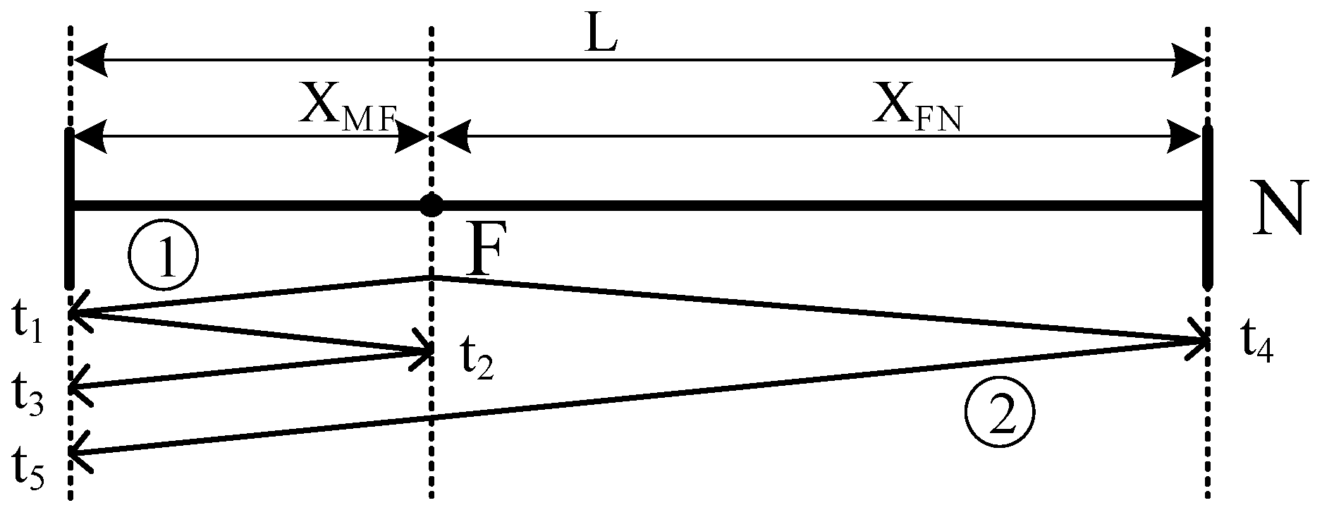
The single-ended method has high real-time performance in calculating measurement results, but it relies on precise hardware equipment. If the wave head cannot be accurately captured, it will lead to significant calculation errors and positioning failures.
Secondly, it is necessary to model and analyze the corresponding lines. This article adopts the Bergeron model shown in Figure 3 to simplify the analysis process. , , , and represent the voltage and current at the M and N terminals of the line, respectively; represents the line’s wave impedance. and are the Bergeron line’s equivalent voltage sources, which may be written as:
In the formula, and are the voltage forward waves at the M and N terminals of the line, respectively, and is the transfer function of the line, where is the propagation coefficient and is the length of the line.
Figure 3.
Bergeron model for DC transmission lines.

Due to capacitive and inductive coupling between the poles in bipolar DC transmission systems, if there is a ground fault at one pole, it will cause overvoltage at the other healthy pole, which will cause overcurrent. Phase mode transformation converts the line to two independent module domain lines to reduce the complexity of the fault analysis process [24]. The DC line model for each module domain is the same as the unipolar DC line model. The formula for phase mode change is:
In the formula, and represents 1 mode voltage and current, respectively; and represents 0 mode voltage and current, respectively; is the positive voltage; is the negative voltage; is the positive current; and is the negative current.
Based on the aforementioned model simplification, the voltage and current changes brought on by the initial propagation of the fault traveling wave from the fault point to the protection are examined for intra-area faults in DC lines and intra-area terminal faults, respectively.
2.2. Analysis of Faults Characteristics
In a two-terminal DC distribution system, if a fault occurs, an additional fault port will be added at the fault point. Using the above simplification method, a simplified 1-mode network model of the faulted line can be obtained, as shown in Figure 4. Where a single-pole ground fault occurs at point , is the fault transition resistance, is the fault additional excitation power, and is the fault point voltage.
The model contains three Bergeron equivalent voltage sources whose values are determined by the forward-traveling wave generated by the faulty port circuit and the transfer function of the line. Before the fault traveling wave propagates to both ends of the line and reflects, and is both zero. Since this chapter only considers the voltage and current changes caused by the first traveling wave of the fault arriving at the protection and does not consider the reflexive behavior after that, only the initial excitation state of the fault needs to be taken into account in the calculation. Further, the model of Figure 4 can be simplified, as shown in Figure 5.
and represent the 1-mode component of the fault voltage and current measured at the protection installation site.
The boundary conditions of the phase domain are [26]:
, , and respectively the DC voltage value at the fault point before the fault, the voltage at the positive fault point, the current at the positive fault point, and the current at the negative fault point.
Furthermore, according to the domain network structure, it can be seen that:
By combining Equations (5) and (6), the complex frequency domain expression of the fault point voltage can be obtained:
Furthermore, the equivalent voltage source of the 1-mode line Bergeron is:
Based on the network structure of the port where the protection is located, calculate the expression of the mode domain voltage and current fault components obtained from the protection measurement using the following formula:
By solving the Laplace inverse transformation for (9) and (10), the time-domain analytical expressions corresponding to modulus voltage and current can be obtained.
Using the same analysis method, obtain the complex frequency domain and time domain analytical expressions of 0 mode voltage and current. Finally, the time-domain solutions of phase-domain voltage and current fault components are calculated using phase-mode inverse transformation.
2.3. Arc Fault Characterization of DC Systems
Arc faults in DC systems can be categorized into series arc faults and parallel arc faults. In this paper, only parallel arc faults are considered. When a parallel arc fault occurs, the arc is directly connected to the earth or connected to the earth through the medium. The arc resistance is affected by some factors, such as arc voltage, arc current, and gap length.
To simulate the arc fault, the Cassie model was used to simulate the dynamic behavior of the arc burning [27]. Arc resistance is affected by the energy relationship between the arc voltage and arc current.
The heat balance equation for the arc is shown in Equation (11). is the energy stored in the arc. is the dissipated power. and are the arc voltage and arc current, respectively.
Equation (11) can be changed to quantify the relationship between the rate of change of arc unit conductivity and the change of arc power.
Equation (13) represents the arc resistance for the Cassie model, where is the time constant and is the arc voltage gradient.
3. Fault Location Method Based on EMD-SVD
Hilbert Huang (HHT) is a signal processing method based on instantaneous frequency characteristics, proposed by N.E. Huang et al., which can accurately describe the characteristics of signal frequency in the time domain [28].
3.1. Traveling Wave Decomposition with EMD
The EMD process uses mathematical methods to construct an envelope, which envelopes all of the data in the signal . The envelope is then computed by subtracting the average from the original signal and subtracting the residual component. The mean of the envelope is then calculated, and the mean is subtracted from the original signal to obtain the residual component .
If meets the conditions defined by the IMF, then it is taken as the first component. If it does not meet the conditions defined by the IMF, then use it as the original signal and repeat steps 1 and 2 until the first component is obtained.
After separating , the remaining signal is obtained. Repeat the above steps to obtain the 2, 3, 4, ... nth IMF components in sequence. If the function obtained from the last decomposition meets the IMF definition, the loop ends. The above decomposition process can be simplified, as shown in Figure 6.
In the EMD process, the IMF components are extracted in order from high frequency to low frequency. is the signal with the highest frequency; is the signal with the lowest frequency and represents the average trend of the signal. This set of IMF components is all single-component signals, i.e., each moment contains only one frequency component.
For any time-series signal , define its Hilbert transform as [28]:
Its inverse transformation is:
In the formula, represents the principal value, and represents time. and are mutually complex conjugates. The expression of the analytic signal is:
Among them:
In the formula, represents the instantaneous amplitude and represents the instantaneous phase. Given the phase, the instantaneous frequency can be calculated utilizing the following formula:
Often, the instantaneous phase and instantaneous frequency obtained by directly performing the Hilbert transform on the signal will have meaningless negative values because most signals do not only contain one vibration mode but are composed of multiple complex waves superimposed (the signal is locally asymmetric to the zero means). The premise of performing the Hilbert transform is to perform EMD on the signal to obtain a series of stable IMF with only one vibration mode. The accuracy of the time synchronization when the traveling wave head reaches the measurement point seriously affects the accuracy of the traveling wave method for distance measurement. When the fault traveling wave propagates to the measurement point, the signal detected by the measuring point shows a high-frequency mutation, and the mutation point marks the arrival time of the fault traveling wave. The characteristic of high-frequency sudden changes in the time-frequency map of the traveling wave signal head allows the time corresponding to the first frequency sudden change point in the instantaneous frequency map to be regarded as the time when the fault traveling wave head reaches the measurement point.
The first intrinsic modal function () of the signal EMD is the component with the highest frequency and has a high temporal resolution. Therefore, the moment when the faulty wave head arrives at the measurement point can be determined by the mutation point in the time-domain plot of this component.
3.2. Traveling Wave Head Calibration with SVD
Singular value decomposition (SVD) is a mathematical method of orthogonal transformation, as shown in Equation (21). Where A is an arbitrary real matrix, and are orthogonal matrices of order m and n, respectively, and matrix is a diagonal matrix whose diagonal elements are composed of singular values, Through SVD, matrix can be decomposed into a superposition of a principal component and several detail components, with each singular value corresponding to a component. This decomposition ensures that the phase of each component is the same.
Given a discrete signal , if it is constructed into a Hankel matrix, SVD can be used to achieve singularity detection of the signal, that is, to detect sudden changes in the signal itself or its derivative at a certain moment. The Hankel matrix form is:
Construct signal as a Hankel matrix and perform SVD, where the matrix can be represented as:
Through Equation (23), signal reconstruction can be performed on each SVD component: . The elements in are the combination of the elements of the first column and the last row in the matrix .
The component is the main component of the original signal , which approximates the original signal; the component is the detail component of the signal , which can detect the signal itself and the singularity of a certain order derivative of the signal. If we take the mode value of the first detail component, the moment corresponding to the mode maximum point is the moment of signal mutation.
The traveling wave method for distance measurement relies on accurate measurement of the time when the fault traveling wave head reaches the monitoring point. When a fault occurs in a certain part of a DC transmission line, the initial fault traveling wave propagates from the fault point to the monitoring points at both ends of the line. The voltage and current signals detected by the monitoring points show high-frequency mutations in the time-frequency map, and the mutation point marks the time when the fault traveling wave reaches the detection point. Due to the high-frequency mutation of the traveling wave signal head in the time-frequency map, the time corresponding to the first frequency mutation point in the instantaneous frequency graph can be considered the time when the fault traveling wave head reaches the monitoring point.
From the analysis in Section 3.1, it is known that the first eigenmode function of the signal EMD is the highest frequency component with high temporal resolution. Therefore, the time at which the faulty traveling wave head arrives at the monitoring point can be determined by the mutation point in the time-frequency diagram of the component.
The locating steps in this paper are as follows: EMD is performed on the fault current signal; the highest frequency component is taken and its Hankel matrix is constructed; the constructed Hankel matrix is decomposed into two layers of singular values, the first one being the main component and the second one being the detail component; the detail component detects the singularity of the component itself. Take the mode value of the detail component; the maximum value of the mode value is the first mutation point of the component, and the corresponding time is the time when the initial traveling wave head reaches the monitoring point for the first time; the second maximum value of the mode value corresponds to the time when the initial traveling wave is reflected back to the monitoring point again by the fault point; in this way, we can realize the calibration of the wave head of the faulty traveling wave. At last, the time required is substituted into the distance measurement formula in Equation (2) to obtain the distance measurement results. The locating process described above can be represented by Figure 7.
4. Case Study
4.1. DC Distribution Network Modeling
Based on the PSCAD simulation platform, the simulation model of the double-ended DC distribution network shown in Figure 8 is established.
The length of the line is 20 km using an XLPE cable, and the line voltage is ±10 kV. MMC (modular multilevel converter) is used for both the sender-end rectifier and the receiver-end inverter. The fault type is set as DC arc fault. The simulation duration is 3.5 s, and the fault occurs at a moment of 3 s with a duration of 0.1 s. The simulation sampling frequency is 1 MHz.
In the system, the block diagram of the converter control strategy is shown in Figure 9. The inverter at the receiving-end operates in a constant DC voltage and constant reactive power control mode, controlling the DC voltage of the system based on the voltage value provided by the DC distribution system, providing a voltage reference value for the entire DC distribution network and providing reactive power support to the AC side when required. The sending-end rectifier uses constant active and reactive power control to control the flow of power. This control strategy regulates both the distribution system power and the DC voltage.
In the locating algorithm, the traveling wave velocity is fixed using XLPE cable as the reference wave velocity m/s, where is the speed of light. and are the relative dielectric constant and relative magnetic conductivity of XLPE, the insulation material for DC cables, , ).
4.2. Locating Results
Analyze the positive current data within 0.002 s before and after the fault occurred at the sending-end detection point. As depicted in Figure 10, the system is in stable operation prior to the occurrence of a fault; following the occurrence of a fault, the high-frequency fault traveling wave signal propagates along the line to the sending end, and the current at the monitoring point at the sending end experiences a sudden change.
As shown in Figure 11, EMD is conducted on the positive sender current signal to get the component with the highest frequency in the IMF cluster. The current amplitude tends to decrease with the propagation of the faulty traveling current on the line and the fold-reflection behavior.
From the analysis in Chapter III, it can be seen that SVD can detect the singularities of the signal itself and its derivatives. In order to obtain the mutation points of the component, two layers of singular value decomposition are used in this paper. The main component reflects the main frame of the signal, and the detail component can detect the mutation points of the signal itself. As shown in Figure 12, the detail component’s maximum modulus point corresponds to the component’s mutation point.
Take the modulus value of the svd2 component, as shown in Figure 13, where ① is the first modulus maximum point, and its corresponding time represents the time when the initial fault traveling wave current propagates from the fault point to the sending-end monitoring point, and ② is the second modulus maximum point, and its corresponding time represents the time when the initial fault traveling wave current returns to the monitoring point after being refracted twice by the sending-end bus and the fault point. The distance from the fault point to the monitoring point at the sending end can be obtained by substituting the two time points into the ranging formula to achieve fault location.
Based on the above ranging scheme, several groups of different fault locations were set up for the experiments. Table 1 and Table 2 show the results of single-end ranging experiments with faults set near the line midpoint and at the end of the line, respectively.
In Table 1, X is the actual fault point, and the initial fault traveling wave propagates to the sending-end measurement point for the first time along the line at TM1 time; After two refractions of the bus and fault point, it reaches the sending-end measurement point again at TM2 time. XM is the distance calculation result from the fault position to the sending-end monitoring point, and XR is the ranging error.
In addition, the ranging errors for more fault points are shown as a scatter plot in Figure 14. The error range over the entire line is between 0.055% and 1.157%. Obviously, the proposed locating scheme did not fail when the fault occurred close to the end of the line.
4.3. Effect of Transition Resistance
The effectiveness of the proposed scheme is verified in different transition resistance cases, respectively.
As shown in Figure 15, in the case of a low transition resistance, the amplitude of the wave head is large and easy to identify; with the increase of the transition resistance, the peak value of the wave head gradually decreases, the reflected wave head is difficult to identify, and the single-ended method of traveling wave ranging scheme faces failure. So, for high-resistance faults, the traveling wave method faces challenges.
4.4. Comparative Study of Different Signal Processing Methods
Currently, there are many methods for processing faulty traveling wave signals in the time-frequency domain. For example, EMD is used in this paper, as well as CEEMD, CEEMDAN, VMD, etc. EMD algorithms may suffer from end-point effects as well as modal aliasing when decomposing time-domain signals. Many scholars have further improved on the basis of EMD to solve the possible problems of EMD. To address this, we conducted a comparative study of the above algorithms for fault localization.
As shown in Figure 16, CEEMD and CEEMDAN add Gaussian white noise to the original signal to resolve the modal aliasing phenomenon of EMD; however, the high-frequency Gaussian white noise still remains in the intrinsic mode function of the signal, resulting in a large fluctuation of the component and making it difficult to locate the second peak point. Unlike EMD, the VMD method constrains the bandwidth of the eigenmode functions so that the frequency of each eigenmode function is around a center frequency, similar to a band-pass filter; however, this method also affects the identification of the wave head. In addition, the signal is decomposed by different methods, and the EMD decomposition has a much better advantage in terms of wave amplitude than the other methods.
5. Conclusions
In this paper, based on a single-ended traveling wave locating principle, a combined EMD-SVD method is proposed to realize the calibration of the fault traveling wave head. A ±10 kV DC distribution network model is built in PSCAD V4.6 simulation software, and the reliability and accuracy of the algorithm are verified in MATLAB R2021b.
The locating results show that the scheme can well extract the high-frequency fault traveling wave signal and calibrate the arrival moment of the traveling wave head, and the ranging error range of the whole line is between 0.055% and 1.157%, which has a high ranging accuracy. In addition, in a comparative study with other schemes, it was found that the high-frequency signal extracted by EMD is smoother and has a larger wave amplitude, and there are obvious wave peaks only at the mutation points, which is more conducive to the realization of fault localization. However, facing the challenge of high resistance, when the transition resistance is large, the wave amplitude decreases sharply, and it may not be able to identify the wave head and the localization failure.
The following factors primarily affect the accuracy of the proposed scheme in this paper:
- (1)
- Wave velocity. The article uses the empirical wave speed and substitutes it into the ranging formula to calculate the fault distance. However, in reality, traveling wave propagation in the line does not propagate at a fixed wave speed, and the use of a fixed wave speed to calculate will inevitably cause a certain error.
- (2)
- The algorithm itself. The EMD algorithm, in the process of decomposition of the signal, may appear to have modal aliasing and an endpoint effect. The EMD decomposition process is from high-frequency to low-frequency decomposition, the highest frequency component priority separation. In this paper, we use the highest frequency component of EMD and focus more on the abruptness of the signal. The degree of influence of the algorithm is minimized. However, further improvement of the algorithm may improve the accuracy of the experimental results.
Finally, although the traveling wave method has the phenomenon of sensitivity to transition resistance, it has received attention for its higher accuracy and faster speed. The study in this paper verifies the feasibility of the traveling wave method for use in DC distribution networks as well as its ranging accuracy. In view of the influencing factors, we will focus on the influence of traveling wave speed, improve the application of the EMD algorithm in traveling wave ranging in subsequent research, and promote the development of hardware platforms.
Author Contributions
L.J. supervised the study and coordinated the main theme of this paper. L.X. prepared the manuscript and completed the simulations. T.Z. and J.Z. discussed the results and implications and commented on the manuscript. All authors have read and agreed to the published version of the manuscript.
Funding
Project supported by the National Key R&D Program of China (2021YFE0103800).
Institutional Review Board Statement
Not applicable.
Informed Consent Statement
Not applicable.
Data Availability Statement
The data used to support the findings of this study are available from the corresponding author upon request.
Conflicts of Interest
The authors declare no conflict of interest.
References
- Wei, W.; Zhou, Y.; Zhu, J.; Hou, K.; Zhao, H.; Li, Z.; Xu, T. Reliability Assessment for AC/DC Hybrid Distribution Network with High Penetration of Renewable Energy. IEEE Access 2019, 7, 153141–153150. [Google Scholar] [CrossRef]
- Xiao, J.; Zhang, Y.; Wan, L.; Li, H. Application of DC Grid in Global Energy Internet Positioning and Case Study. Glob. Energy Internet 2018, 1, 32–38. [Google Scholar]
- Shen, M.; Zhou, S.; An, Z.; Wang, T. Influence of Distributed Photovoltaic Access on Power Quality of Distribution Network and Countermeasures in New Power System. In Proceedings of the 18th International Conference on AC and DC Power Transmission (ACDC 2022), Online Conference, 2–3 July 2022; pp. 919–924. [Google Scholar]
- Elsayed, A.T.; Mohamed, A.A.; Mohammed, O.A. DC Microgrids and Distribution Systems: An Overview. Electr. Power Syst. Res. 2015, 119, 407–417. [Google Scholar] [CrossRef]
- Zhang, W.; Liang, H.; Bin, Z.; Li, W.; Guo, R. Review of DC Technology in Future Smart Distribution Grid. In Proceedings of the IEEE PES Innovative Smart Grid Technologies, Tianjin, China, 16–20 January 2012; pp. 1–4. [Google Scholar]
- Zhan, C.; Smith, C.; Crane, A.; Bullock, A.; Grieve, D. DC Transmission and Distribution System for a Large Offshore Wind Farm. In Proceedings of the 9th IET International Conference on AC and DC Power Transmission (ACDC 2010), London, UK, 19–21 October 2010; pp. 1–5. [Google Scholar]
- Masrur, M.A.; Skowronska, A.G.; Hancock, J.; Kolhoff, S.W.; McGrew, D.Z.; Vandiver, J.C.; Gatherer, J. Military-Based Vehicle-to-Grid and Vehicle-to-Vehicle Microgrid—System Architecture and Implementation. IEEE Trans. Transp. Electrif. 2018, 4, 157–171. [Google Scholar] [CrossRef]
- He, J.; Zhou, J.; Zheng, F.; Xia, Y.; Yuan, W. Application of AC/DC Hybrid System in Industrial Park Scenario. In Proceedings of the 2020 Asia Energy and Electrical Engineering Symposium (AEEES), Chengdu, China, 29–31 May 2020; pp. 978–982. [Google Scholar]
- Gururajapathy, S.S.; Mokhlis, H.; Illias, H.A. Fault Location and Detection Techniques in Power Distribution Systems with Distributed Generation: A Review. Renew. Sustain. Energy Rev. 2017, 74, 949–958. [Google Scholar] [CrossRef]
- Gong, B.; Fan, L.; Li, R.; Zhu, D.; Zeng, C.; Jia, Y.; Lan, Y.; Xu, S. Mechanism Analysis of Mountain Fire Caused by Arc Grounding Fault Discharge in Distribution Network in Forest and Pastoral Areas. In Proceedings of the 2023 6th International Conference on Energy, Electrical and Power Engineering (CEEPE), Guangzhou, China, 12–14 May 2023; pp. 1140–1145. [Google Scholar]
- Wang, Z.; Balog, R.S. Arc Fault and Flash Signal Analysis in DC Distribution Systems Using Wavelet Transformation. IEEE Trans. Smart Grid 2015, 6, 1955–1963. [Google Scholar] [CrossRef]
- Heng, N.; Liang, K. Review on Fault Protection Technologies do DC Microgrid. High Volt. Technol. 2020, 46, 2241–2254. [Google Scholar]
- Zhang, M.; Guo, R.; Sun, H. Fault Location of MMC-HVDC DC Transmission Line Based on Improved VMD and S Transform. In Proceedings of the 2020 4th International Conference on HVDC (HVDC), Xi’an, China, 6–9 November 2020; pp. 792–796. [Google Scholar]
- Yu, L.; Zou, G.; Wei, X.; Sun, C. Traveling Wave Bus Protection for MMC Based Multi-terminal DC Distribution Network. In Proceedings of the 2019 IEEE 8th International Conference on Advanced Power System Automation and Protection (APAP), Xi’an, China, 21–24 October 2019; pp. 373–377. [Google Scholar]
- Li, B.; He, J.; Li, Y.; Li, B.; Wen, W. High-speed Directional Pilot Protection for MVDC Distribution Systems. Int. J. Electr. Power Energy Syst. 2020, 121, 106141. [Google Scholar] [CrossRef]
- Zhang, X.; Tai, N.; Wang, Y. EMTR-Based Fault Location for DC Line in VSC-MTDC System Using High-Frequency Currents. Iet Gener. Transm. Distrib. 2017, 11, 2499–2507. [Google Scholar] [CrossRef]
- Elgamasy, M.M.; Izzularab, M.A.; Zhang, X.-P. Single-End Based Fault Location Method for VSC-HVDC Transmission Systems. IEEE Access 2022, 10, 43129–43142. [Google Scholar] [CrossRef]
- Yang, Y.; Huang, C.; Xu, Q. A Fault Location Method Suitable for Low-Voltage DC Line. IEEE Trans. Power Deliv. 2020, 35, 194–204. [Google Scholar] [CrossRef]
- Park, J.-D.; Candelaria, J.; Ma, L.; Dunn, K. DC Ring-Bus Microgrid Fault Protection and Identification of Fault Location. IEEE Trans. Power Deliv. 2013, 28, 2574–2584. [Google Scholar] [CrossRef]
- Liu, W.; Liu, F.; Zha, X.; Huang, M.; Chen, C.; Zhuang, Y. An Improved SSCB Combining Fault Interruption and Fault Location Functions for DC Line Short-Circuit Fault Protection. IEEE Trans. Power Deliv. 2019, 34, 858–868. [Google Scholar] [CrossRef]
- Jia, K.; Shi, Z.; Wang, C.; Li, J.; Bi, T. Active Converter Injection-Based Protection for a Photovoltaic DC Distribution System. IEEE Trans. Ind. Electron. 2022, 69, 5911–5921. [Google Scholar] [CrossRef]
- Huang, N.E.; Shen, Z.; Long, S.R.; Tung, C.C.; Liu, H.H. The Empirical Mode Decomposition and Hilbert Spectrum for Nonlinear and Non-stationary Time Series Analysis. Proc. R. Soc. Lond. A 1998, 454, 903–995. [Google Scholar] [CrossRef]
- Ren, W.; Song, J.; Tian, S.; Zhang, X. Estimation of the Equivalent Number of Looks in SAR Images Based on Singular Value Decomposition. IEEE Geosci. Remote Sens. Lett. 2015, 12, 2208–2212. [Google Scholar] [CrossRef]
- Dong, X. The Theory of Fault Travel Waves and Its Application; Springer: Singapore, 2022. [Google Scholar]
- Shang, L.; Zhai, W.; Liu, P. Study of Fault Location in Transmission Line Using S Transform. In Proceedings of the 2016 International Symposium on Computer, Consumer and Control (IS3C), Xi’an, China, 4–6 July 2016. [Google Scholar]
- Li, A.; Cai, Z.; Li, X. Study on the Propagation Characteristics of Traveling Waves in HVDC Transmission Lines on the Basis of Analytical Method. Chin. J. Electr. Eng. 2010, 30, 94–100. [Google Scholar]
- Jalil, M.; Samet, H.; Ghanbari, T.; Tajdinian, M. An Enhanced Cassie–Mayr-Based Approach for DC Series Arc Modeling in PV Systems. IEEE Trans. Instrum. Meas. 2021, 70, 9005710. [Google Scholar] [CrossRef]
- Li, X.; Jin, J.; Shen, Y.; Liu, Y. Noise level estimation method with application to EMD-based signal denoising. J. Syst. Eng. Electron. 2016, 27, 763–771. [Google Scholar]
Figure 1.
Post-fault network decomposition. (a) Post-fault network. (b) Normal network. (c) Fault component network.
Figure 1.
Post-fault network decomposition. (a) Post-fault network. (b) Normal network. (c) Fault component network.
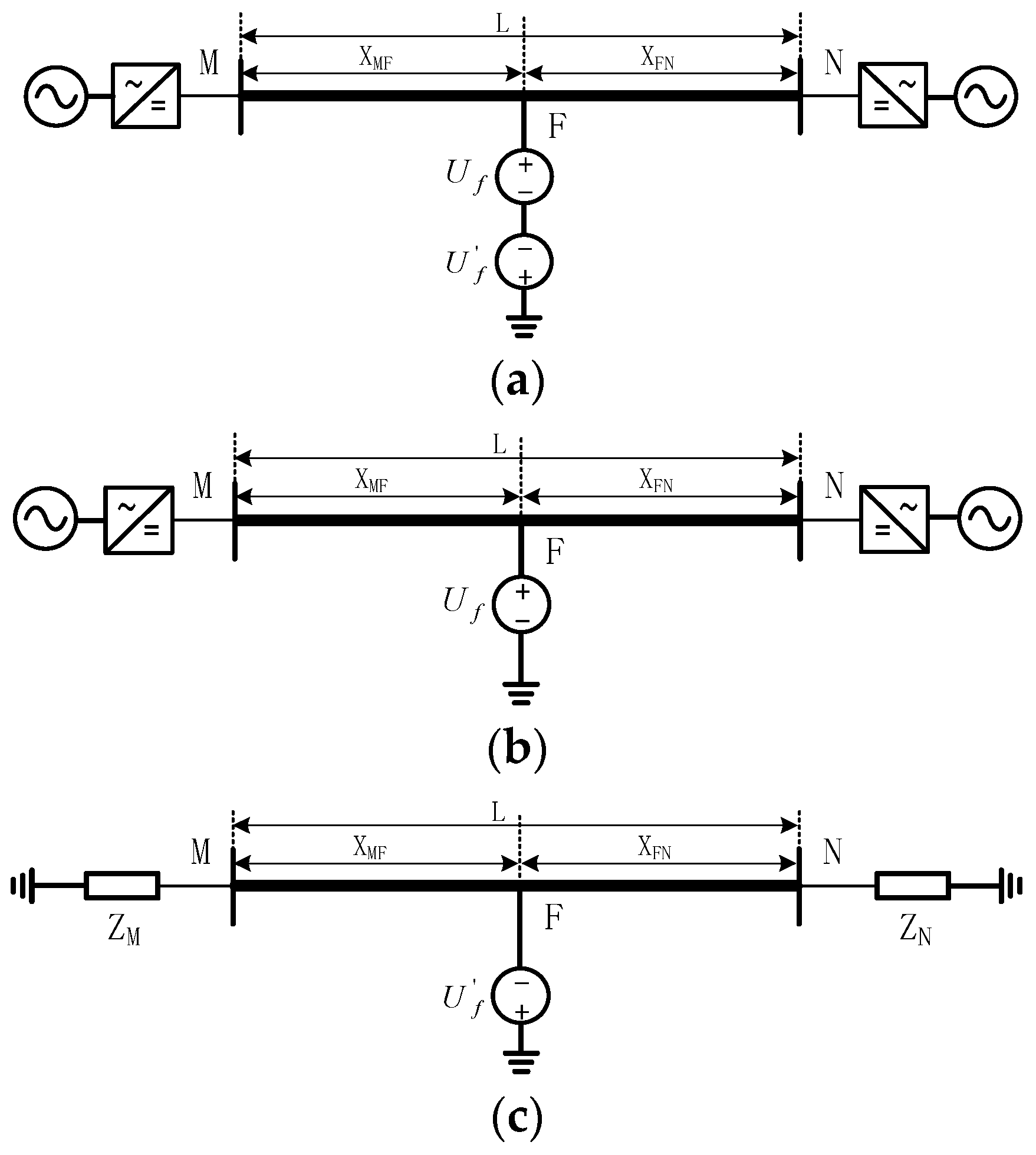
Figure 4.
A simplified model of a double terminal DC system line under fault conditions.
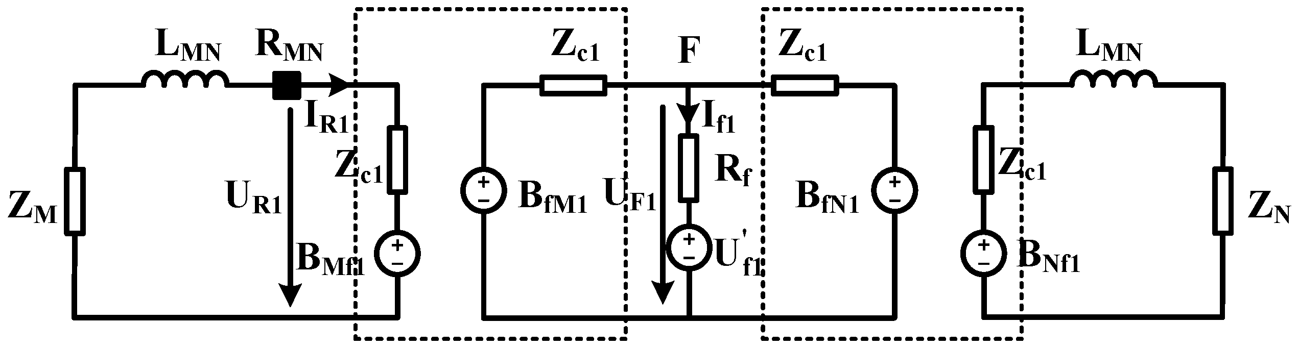
Figure 5.
Minimalist computational model.

Figure 6.
EMD decomposition diagram.

Figure 7.
Traveling wave fault location process based on EMD-SVD.
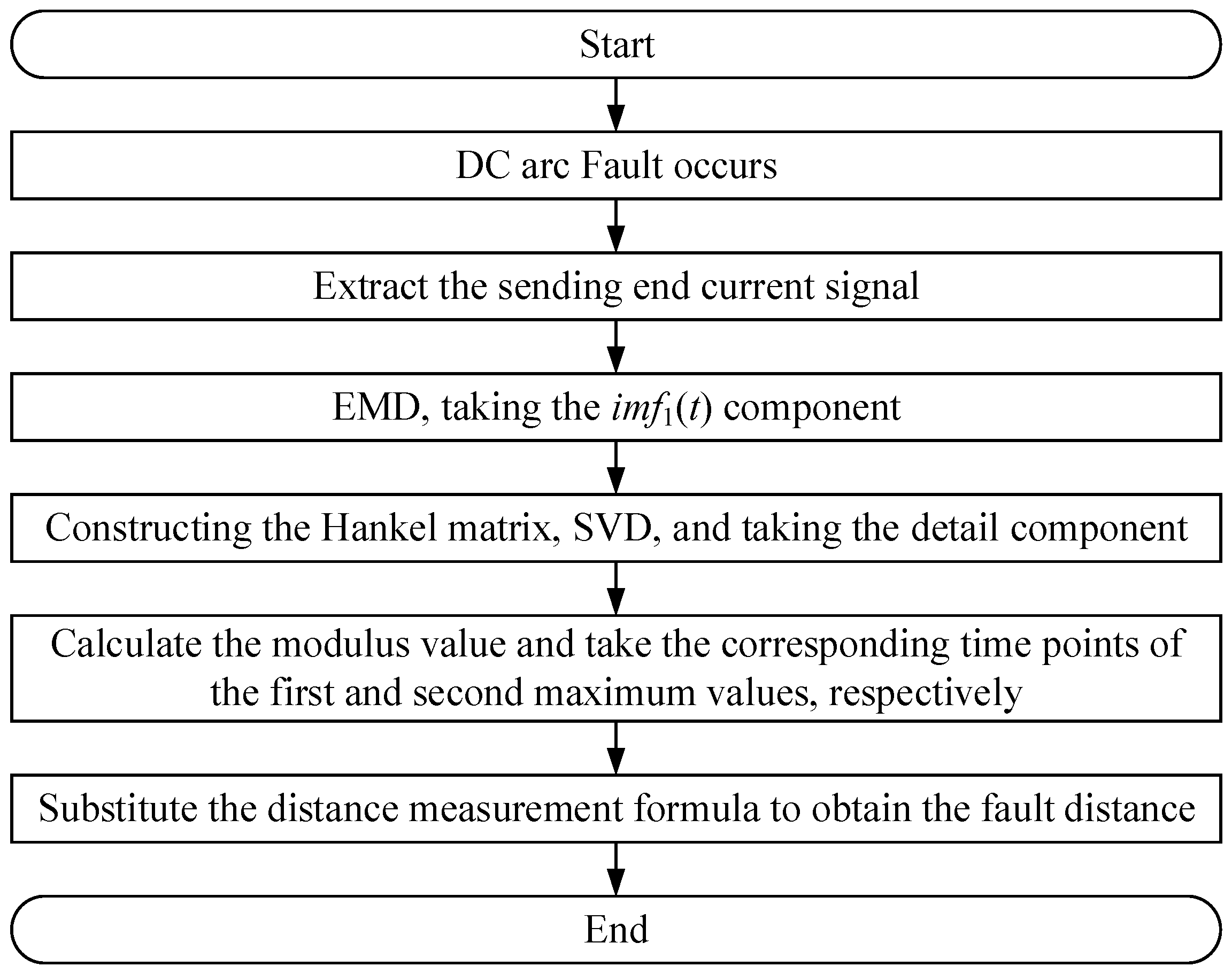
Figure 8.
The topological structure of the simulation model.
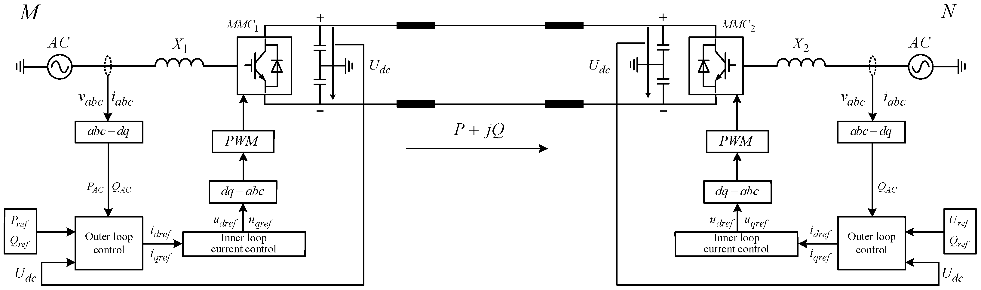
Figure 9.
Schematic diagram of the converter control strategy. (a) Schematic diagram of the control strategy at the delivery end. (b) Schematic diagram of the control strategy at the receiving end.
Figure 9.
Schematic diagram of the converter control strategy. (a) Schematic diagram of the control strategy at the delivery end. (b) Schematic diagram of the control strategy at the receiving end.
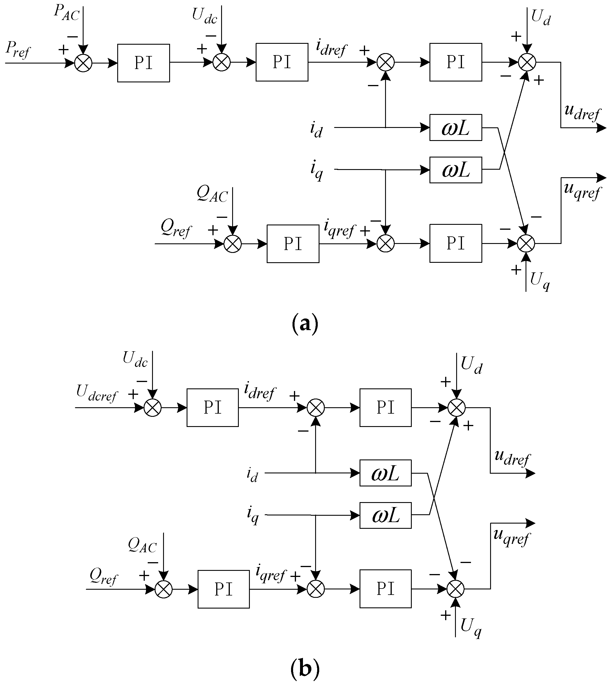
Figure 10.
Positive current at the sending end.
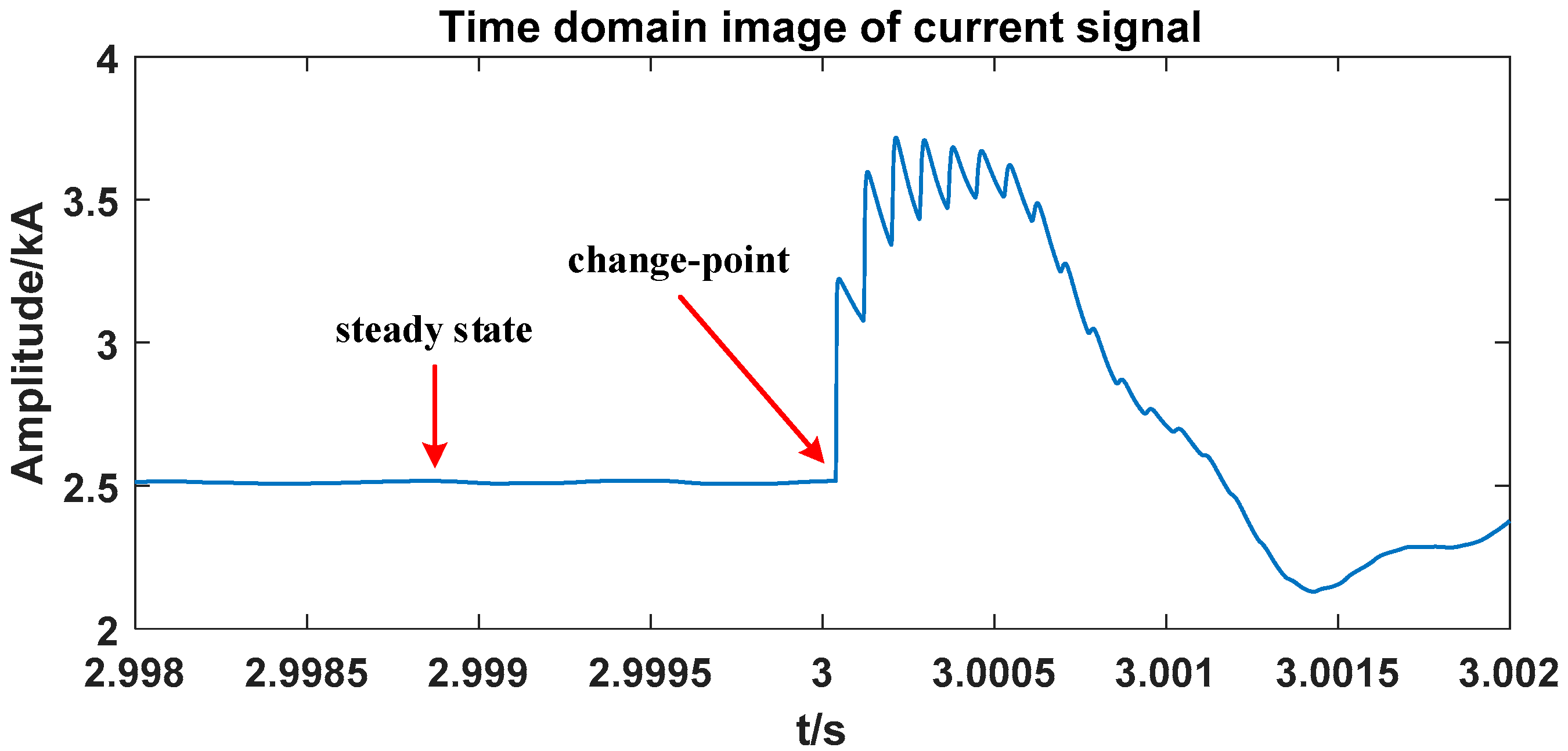
Figure 11.
Component.

Figure 12.
Component and its svd2 component.
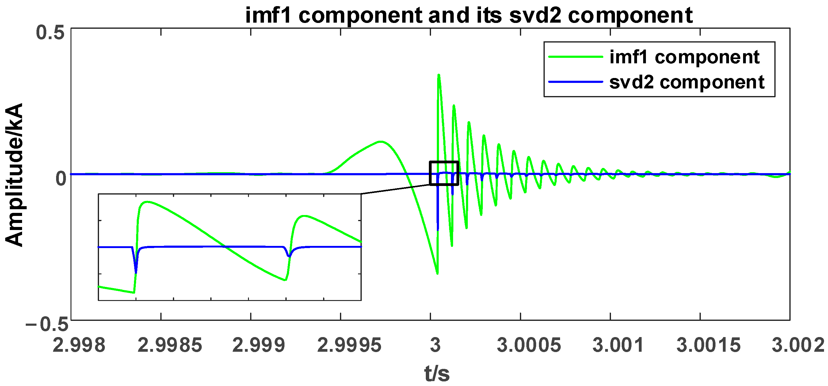
Figure 13.
Modulus of svd2 components. ① First maximum value. ② Second maximum value.

Figure 14.
Scatterplot of locating error.
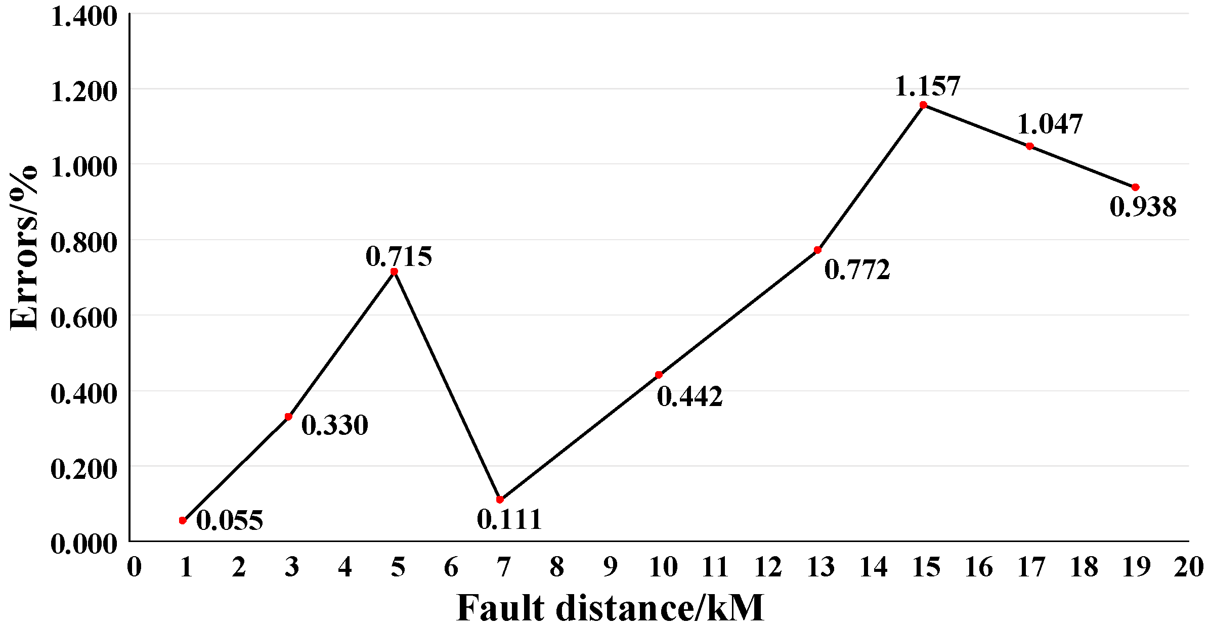
Figure 15.
Schematic of SVD detail components with different transition resistances.

Figure 16.
Wave head identification with different signal processing methods. (a) Full view. (b) Expanded view.
Figure 16.
Wave head identification with different signal processing methods. (a) Full view. (b) Expanded view.


Table 1.
Distance measurement results of fault location near the midpoint of the line.
| X/km | TM1/s | TN2/s | XM/km | XR/% |
|---|---|---|---|---|
| 5 km from M end, 15 km from N end | 3.000024 | 3.000076 | 5.143060 | 0.715 |
| 10 km from M end, 10 km from N end | 3.000051 | 3.000153 | 10.088310 | 0.442 |
| 15 km from M end, 5 km from N end | 3.000076 | 3.000230 | 15.231370 | 1.157 |
Table 2.
Distance measurement results of fault location at the end of the line.
| X/km | TM1/s | TN2/s | XM/km | XR/% |
|---|---|---|---|---|
| 1 km from M end, 19 km from N end | 3.000004 | 3.000014 | 0.989050 | 0.055 |
| 19 km from M end, 1 km from N end | 3.000097 | 3.000291 | 19.187570 | 0.938 |
Disclaimer/Publisher’s Note: The statements, opinions and data contained in all publications are solely those of the individual author(s) and contributor(s) and not of MDPI and/or the editor(s). MDPI and/or the editor(s) disclaim responsibility for any injury to people or property resulting from any ideas, methods, instructions or products referred to in the content. |
© 2023 by the authors. Licensee MDPI, Basel, Switzerland. This article is an open access article distributed under the terms and conditions of the Creative Commons Attribution (CC BY) license (https://creativecommons.org/licenses/by/4.0/).
Share and Cite
MDPI and ACS Style
Jing, L.; Xia, L.; Zhao, T.; Zhou, J. An Improved Arc Fault Location Method of DC Distribution System Based on EMD-SVD Decomposition. Appl. Sci. 2023, 13, 9132. https://doi.org/10.3390/app13169132
AMA Style
Jing L, Xia L, Zhao T, Zhou J. An Improved Arc Fault Location Method of DC Distribution System Based on EMD-SVD Decomposition. Applied Sciences. 2023; 13(16):9132. https://doi.org/10.3390/app13169132
Chicago/Turabian StyleJing, Liuming, Lei Xia, Tong Zhao, and Jinghua Zhou. 2023. "An Improved Arc Fault Location Method of DC Distribution System Based on EMD-SVD Decomposition" Applied Sciences 13, no. 16: 9132. https://doi.org/10.3390/app13169132
Note that from the first issue of 2016, this journal uses article numbers instead of page numbers. See further details here.