Prediction of Ground Movements and Impacts on Adjacent Buildings Due to Inclined–Vertical Framed Retaining Wall-Retained Excavations

Featured Application

This article presents a prediction method for the displacement of the soil outside inclined–vertical framed-retaining-wall-retained excavations and evaluates the probability of damage to nearby buildings.

Abstract

Inclined–vertical framed retaining walls were recently developed and successfully adopted in engineering practice. However, relevant empirical methods for the evaluation of ground movements due to excavation have not been established. This study aimed to establish a calculation method for assessing ground movement due to excavation and to evaluate the damage probability of nearby buildings. A series of numerical models were carried out, and a database was established with their results. In this paper, simplified equations are proposed for predicting the profiles of subsurface and surface settlements, as well as lateral movements, utilizing the database. The accuracy of the simplified equations was validated by monitoring data from three case histories of the inclined–vertical framed retaining wall. Finally, the damage potential index was used to obtain the probability of damage to buildings located outside the excavations, while considering different positions.

1. Introduction

Excavation-induced ground movements are generally unavoidable, thereby affecting adjacent existing buildings. In soft-soil areas, the deformation of excavation is relatively large. Its impact range can reach 3–4 times the depth of the excavation, far greater than the deformation and impact range in hard soil [1,2]. The prediction of ground movements outside/around excavations is crucial, as it can be used to evaluate the influence of the excavation on nearby constructions and ensure safety.

Peck [1] collected a large number of measured data on surface settlement caused by excavations and developed a settlement curve for the surface soil layer. Clough and O’Rourke [3] expanded this measured dataset base and proposed a dimensionless settlement envelope of the ground surface. Hsieh and Ou [2] proposed a surface settlement model for cantilever walls and braced excavations, and they proposed the concept of primary and secondary influence zones. Ou et al. [4] extended the surface settlement curve of braced excavations to the subsurface and proposed lateral displacement curves for different depths. In practice, Li et al. [5] developed the servo struts to control the excavation-induced ground settlement and analyzed the relationship between the strut position and the effectiveness of settlement controlling through field measurements.

To compensate for the limitations of field measurements in terms of monitoring point layout, some articles have conducted research through numerical simulations [6,7,8,9,10,11,12]. Kung et al. [13] used a numerical simulation to propose a calculation equation for the maximum surface settlement of braced excavations. Fan et al. [14] proposed a closed-form solution for the prediction of excavation-induced ground settlement profiles. The profile was derived by assuming the distribution pattern of wall deflection and displacement boundaries. Russo et al. [15] fitted functions by combining longitudinal and transversal settlement troughs based on computed results and evaluated the influence of typical buildings in the subsidence area.

The deformation of a building can be calculated based on the ground movement induced by excavation. As shown in Figure 1, the considered deformations are mainly angular distortion (β) and lateral extension strain (ε_l). Son et al. [16] further simplified the building damage assessment criteria and proposed the damage potential index (DPI), which is calculated according to the angular distortion, β, and the lateral extension strain, ε_l, to evaluate building damage. Ou et al. [4] proposed that using the ground movement of the building foundation burial plane to evaluate building damage is a more accurate way to reflect the actual conditions. The evaluation of ground movement and potential damage to adjacent buildings of embedded walls and braced excavations were substantially discussed.

Zheng et al. [17] reported a new strut-free retaining-wall system called the inclined–vertical framed retaining wall (IVFRW) for deep excavation which consists of three main components: vertical piles, inclined piles, and a capping beam. The inclined piles are laid out counterclockwise from the head of the vertical pile at an angle, α. Through the capping beam, the vertical and inclined piles are connected at the pile head, forming a framed retaining system. The retaining system has been effectively utilized in practical engineering applications, and its wall deformation performance and optimal inclination angle have been studied [18,19]. However, the analysis of the excavation-induced ground movement of IVFRW and its impact on adjacent buildings is limited.

This paper aims to propose a simplified method to predict excavation-induced ground movement with IVFRWs, including the settlement of the ground surface and subsurface and the lateral movement of the ground surface and subsurface. A variety of parametric simulations were carried out. A large number of finite element models were used to establish a database considering the following parameters: the excavation depth, the ratio of the wall depth to the excavation depth (λ), the undrained shear strength of soil (S_u/σ’_v), the stiffness of the retaining pile, and the angle of inclination (θ). Finally, the damage potential index was estimated based on the proposed simplified evaluation methods for surface ground movements.

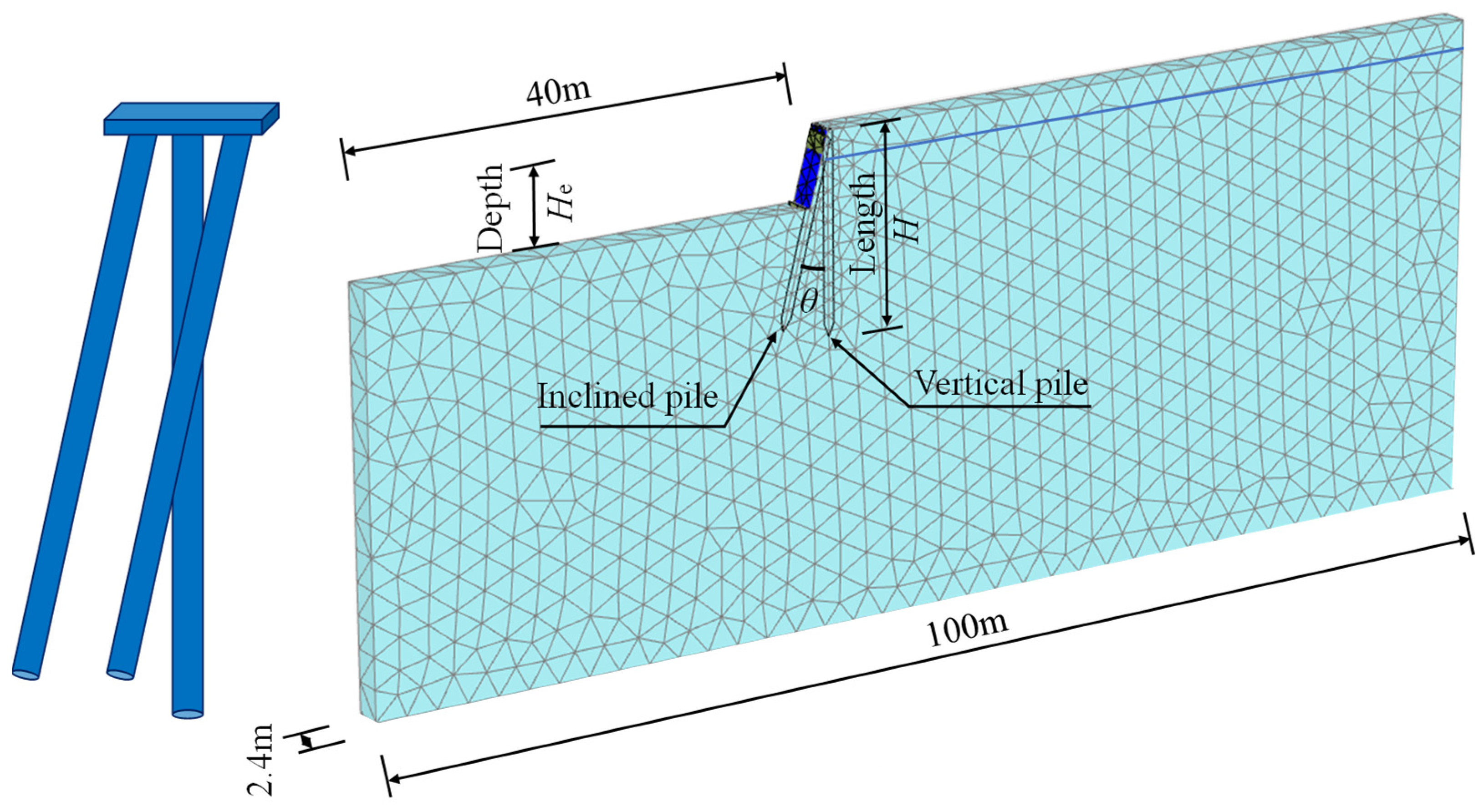
2. Numerical Modeling

An analysis was conducted using a three-dimensional finite element method (FEM) computer program called PLAXIS 3D. To avoid overestimation of retaining structure deformation and ground settlement, the small-strain stiffness of the soil was taken into account [18,19,20]. For this purpose, a hardening soil with a small-strain (HSS) model [21] was adopted for analysis.

2.1. Validation of the Numerical Model

A case history of an excavation in Tianjin, China (39.11° N, 117.20° W), utilizing an IVFRW is depicted in Figure 2. The retaining structure form of section E-E adopts a slope and the IVFRW. The excavation depth is 6 m, including a 1 m slope, and the width of the excavation is approximately 80 m. In section E-E, precast concrete piles with 500 mm sections, a 300 mm hollow diameter, and a center-to-center spacing of 1600 mm were used. Both the inclined and vertical piles had a length of 12 m, with the inclined piles inclined at an angle of 20°, as shown in Figure 3. Clinometers (W18, 7 monitoring points) were used to monitor the lateral deformation of the vertical piles. Total stations (DLZ6-1,8 monitoring points) were utilized to monitor the soil settlement at different distances behind the retaining structure.

Figure 4 shows a three-dimensional model of the excavation with inclined–vertical framed retaining walls. The lateral boundaries of the model are fixed horizontally, while the base is fixed both vertically and horizontally. The excavation width is 80 m, and only half of the entire model is considered due to the symmetry along the y-axis. The maximum excavation depth is 6 m. The retaining structure has a length of 12 m. According to the equivalence principle of stiffness, the walls are simulated using plate elements with a thickness of 0.272 m and a weight of 25 kN/m². The walls have a Young’s modulus of 38 GPa and a Poisson’s ratio of 0.2.

The numerical model, utilizing the HSS constitutive model, was created using PLAXIS 3D software (V20). All relevant parameters, except γ_0.7, were determined from laboratory tests conducted on soil samples obtained using a thin-wall sampler. The strength parameters (c’ and φ’) were obtained through triaxial tests [22]. Apart from the strength parameters, the HSS model requires additional parameters for analysis. These parameters include the secant stiffness, $E_{50}^{\mathrm{ref}}$ (obtained from the triaxial compression test); tangent stiffness, $E_{\mathrm{oed}}^{\mathrm{ref}}$ (obtained from the oedometer loading test); unloading/reloading stiffness, $E_{\mathrm{oed}}^{\mathrm{ref}}$ (obtained from the triaxial unloading/reloading test); initial shear stiffness, $G_0^{\mathrm{ref}}$ (obtained from the bender element test); threshold shear strain, γ_0.7, which represents the shear strain at which the secant modulus (G_s) is reduced to 70% of G₀; and effective stress to describe the stress-strain behavior of soil [23,24]. For a detailed explanation, refer to Brinkgreve et al. [25]. Considering the impact of groundwater-level changes on the deformation of the retaining structure during excavation, the undrained simulation type was chosen.

Table 1. Physical and mechanical parameters of the soil.

Soil Layer	Soil Type	Thickness (m)	γ (kN/m3)	c′ (kPa)	φ′ (°)	${\mathit{E}}_{\mathbf{50}}^{\mathbf{ref}}$ (MPa)	${\mathit{E}}_{\mathbf{oed}}^{\mathbf{ref}}$ (MPa)	${\mathit{E}}_{\mathbf{ur}}^{\mathbf{ref}}$ (MPa)	${\mathit{G}}_{\mathbf{0}}^{\mathbf{ref}}$ (MPa)	γ0.7 (10−3)
1-2	Plain fill soil	1.0	17.1	5.0	8.0	4.2	4.2	12.6	36.0	0.2
4-1	Silty clay	2.0	19.3	20.1	18.0	4.2	4.2	12.6	43.2	0.2
6-3	Silt	6.0	19.4	7.0	33.0	8.0	8.0	24.0	65.0	0.2
6-4	Silty clay	4.6	19.0	21.8	17.7	4.5	4.5	20.0	100.0	0.2
8-1	Silty clay	4.9	19.8	24.3	16.2	5.1	5.1	15.3	76.5	0.2
8-2	Silt	1.5	20.1	9.9	32.3	9.7	9.7	45.3	226.5	0.2

provides a summary of the physical and mechanical parameters of the soils.

Figure 5 illustrates the comparison of the ground surface settlement and wall deflection between the field observations and predictions. The lateral deformation and settlement are reasonably predicted. Thus, the computed data are found to be in good agreement with the measured results, indicating that this FEM modeling approach is reliable for further analysis.

2.2. Numerical Models

According to [26,27,28,29], the main factors that influence ground movement include the excavation depth, ratio of the wall depth to the difference between the wall depth and excavation depth (λ), undrained shear strength of the soil (S_u), and stiffness of the retaining piles, as listed in

Table 2. Input-variable values for analysis.

Excavation Depth, He (m)	λ	Su/σ’v	Stiffness, EI (MN·m²/m)	Inclination Angle, θ (°)
4	0.5	0.163	25.3	5
5	0.8	0.222	85.5	10
6	1.0	0.283	202.7	15
7	1.5	0.345	395.8	20
8	2.0	0.410	684.0	25

. The inclined angle of the retaining pile walls (θ) was also considered in this study.

Figure 6 shows the numerical model. A total of 3600 hypothetical excavations were generated by varying the factors listed in Table 2. Among these 3600 cases, some exhibited unrealistic excavation conditions, such as significant deformation. By excluding such unreasonable cases, models with a maximum settlement of the ground surface of less than or equal to 200 mm were considered to establish a simplified evaluation method for excavation-induced ground movements.

3. Prediction of Excavation-Induced Ground Movement

Figure 7 shows the flowchart of the proposed method for predicting ground movement. Based on the database investigated by FEM modeling, equations of maximum settlement for both the surface and subsurface are established by using the least-squares method. Utilizing the average results obtained from the numerical simulations, the equations for the coordinates X and Z of a dimensionless profile for both surface and subsurface settlements are proposed. Similarly, the equations and profile for the surface and subsurface lateral displacements are obtained. Finally, the angular distortion, β, and the lateral extension strain, ε_l, can be obtained, which can be utilized to analyze the impact of IVFRW-retained excavation on nearby buildings.

3.1. Determination and Validation of the Maximum Surface Settlement

The maximum surface settlement (${\delta }_{\mathsf{\theta }\mathrm{vm},0}$) is influenced by the factors $H_{\mathrm{e}},\lambda ,S_{\mathrm{u}}/{\sigma }_{\mathrm{v}}^{\prime }$, EI, and θ. The results of the FEM numerical analyses of the excavations were collected, and the relationships between the maximum surface settlement and inclination angle were obtained by statistical comparison. Figure 8 shows that the exponential function is the most appropriate to simulate the relationship between ${\delta }_{\mathsf{\theta }\mathrm{vm},0}$ and θ.

By applying the least-squares method to the computed results and all the parameters, the maximum surface settlement, ${\delta }_{\mathsf{\theta }\mathrm{vm},0}$, can be derived from the equations below:

$${\delta }_{\mathsf{\theta }\mathrm{vm},0}=(k_1{e}^v+k_2)e^{{ux}_5}$$

(1)

$$\begin{array}{c}v=k_3{x}_1^2+k_4{x}_1+k_5{x}_2^2+k_6{e}_2+k_7{x}_3^2+k_8{x}_3+k_9{x}_4+k_{10}{x}_1{x}_2\\ +k_{11}{x}_1{x}_3+k_{12}{x}_1{x}_4+k_{13}{x}_2{x}_3+k_{14}{x}_2{x}_4+k_{15}{x}_3{x}_4+k_{16}\end{array}$$

(2)

$$u=k_{17}(k_{18}{x}_2+k_{19})(k_{20}{x}_3+k_{21})(k_{22}{x}_4+k_{23})+k_{24}$$

(3)

where v is used to determine the maximum surface settlement, $x_1=\lambda$, $x_2=H_{\mathrm{e}}$, x₃ = S_u/σ’_v, $x_4=\ln (\gamma /EI)$, $x_5=\theta /100$, and = γ is the water density. k₁–k₂₄ are the fitting coefficients: k₁ = 50.1, k₂ = 0.1, k₃ = −1.2, k₄ = −0.3, k₅ = 1.9, k₆ = −1.2, k₇ = −44.9, k₈ = −0.3, k₉ = 0.0, k₁₀ = 2.7, k₁₁ = 0.1, k₁₂ = 6.9, k₁₃ = −0.1, k₁₄ = 4.1, k₁₅ = 3.8, k₁₆ = 5.5, k₁₇ = 0.1, k₁₈ = −0.8, k₁₉ = 11.1, k₂₀ = −0.3, k₂₁ = 0.3, k₂₂ = −13.2, k₂₃ = 1.1, and k₂₄ = −14.2.

Then, the subsurface settlements can be obtained [4]. The maximum settlement at a specific depth, z, can be calculated by the following equation:

$$\frac{{\delta }_{\mathsf{\theta }\mathrm{vm},z}}{{\delta }_{\mathsf{\theta }\mathrm{vm},0}}=k_{25}{x}_6{}^2+k_{26}{x}_6{+k}_{27}$$

(4)

where x₆ = z/H_e; δ_θvm,z is the maximum settlement at a specific depth, z; and k₂₅ = 0.3, k₂₆ = −1.0, and k₂₇ = 1.0.

By selecting the data points not used in the fitting process (2/3 of the data points from the database were used for fitting), the predicted results from the formula are compared with the FEM results, as shown in Figure 9. Almost all data points are within the error range of ±20%, and the determination coefficient, R², is 0.96, which demonstrates the accuracy of the numerical model in predicting the maximum surface settlement.

To ensure the applicability of the formula, a further error analysis was performed by calculating the base function, which is a ratio of the numerical simulation value to the formula calculation value. After fitting the histogram in Figure 10, it was found that the data distribution follows a normal distribution, with a mean of 1.0 and a standard deviation of 0.09, indicating that the formula is effective.

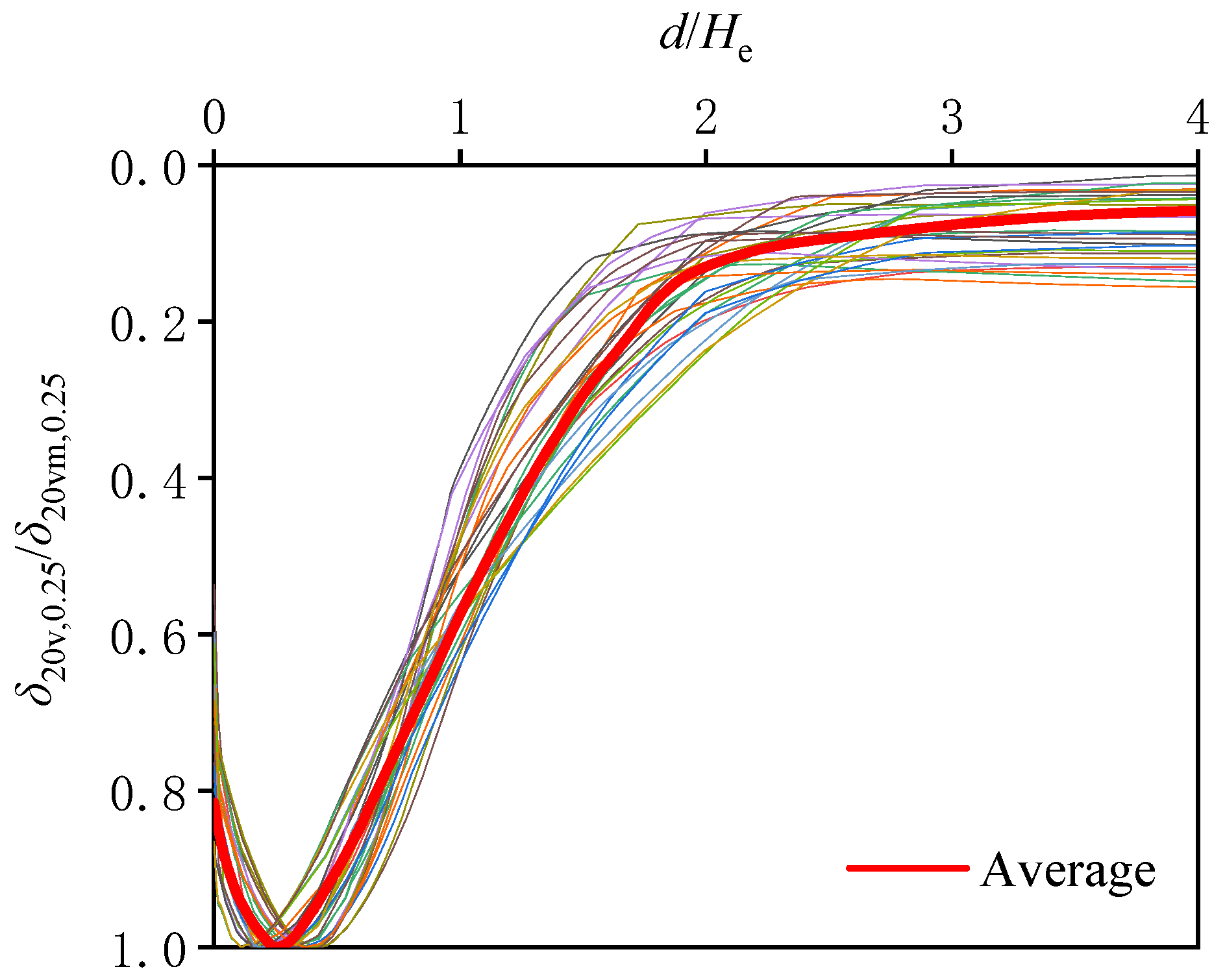
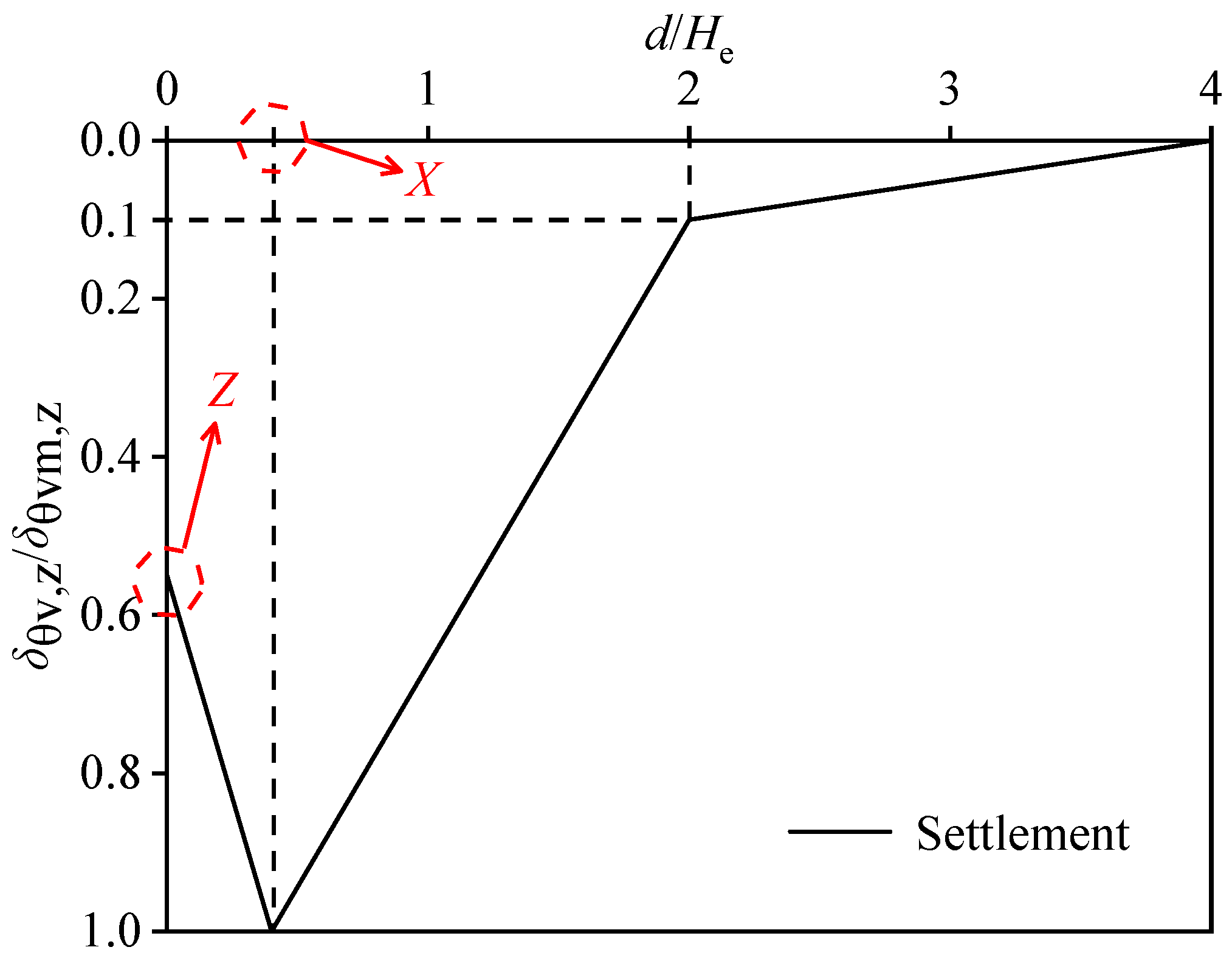
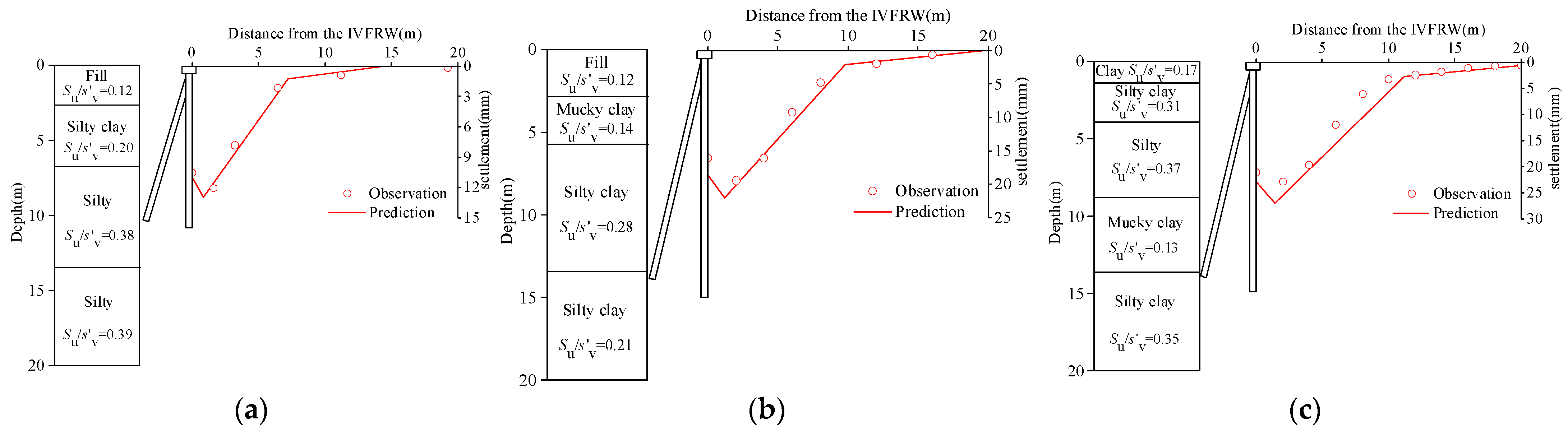
3.2. Determination and Validation of the Settlement Profile

Figure 11 shows the dimensionless curve obtained by taking the average of the settlement with different parameters. Figure 12 shows a dimensionless curve of soil settlement behind the IVFRW. The settlement curve of the IVFRW for different inclination angles is concave, similar to the ground settlement curve of the braced excavations proposed by Hsieh and Ou [2].

The X and Z coordinates in Figure 12 change with the inclination angle and the depth of the soil. With an increase in the inclination angle and the depth of the soil layer, the concave shape of the settlement curve becomes more pronounced. Coordinates X and Z are only related to the inclined pile angles θ and z/H_e and can be expressed as follows:

$$X=k_{28}(e^{k_{29}{x}_5}-1)(k_{30}{e}^{k_{31}{x}_6}-1)$$

(5)

$$Z=k_{32}(e^{k_{33}{x}_5}-1)(k_{34}{e}^{k_{35}{x}_6}-1)+1$$

(6)

where k₂₈ = 1.0, k₂₉ = −8.6, k₃₀ = 0.7, k₃₁ = −0.3, k₃₂ = 2.0, k₃₃ = 0.1, k₃₄ = −2.6, and k₃₅ = 1.0; and the determination coefficients, R², of coordinates X and Z are calculated to be 0.98 and 0.99, respectively.

The deformation mode of the retaining wall and the rotation phenomenon of the principal stress are the reasons why the settlement curve of the soil behind the IVFRW is concave. The deformation mode of the IVFRW is similar to that of braced excavations [17]. The excavation of the IVFRW leads to a principal stress rotation in the soil near the wall. This causes vertical unloading of the soil and results in a concave settlement curve. With increasing depth, the vertical unloading of the soil becomes more pronounced, resulting in a more pronounced concave shape of the settlement curve.

The proposed simplified evaluation method was validated using three IVFRW-retained excavations that provided detailed construction information and measurement data. Figure 13 shows the site plans of the projects and profiles of the sections. Note that, unless otherwise specified, the data in the figure are presented in millimeters. All cases correspond to residential buildings in China, and the areas of the three cases are between 40,000 m² and 50,000 m². The excavation depths of the three cases are 4.5 m, 4.9 m, and 5.6 m, and the lengths of the piles are 11 m, 15 m, and 17 m, respectively. The vertical and inclined piles have identical lengths, and the angle of the inclined piles is 20° for all three cases. Each pile has a rectangular section measuring 0.375 m × 0.5 m, with a hollow diameter of 0.21 m. The center-to-center spacing between adjacent piles of Case 1 is 0.85 m, while the spacing of the other cases is 0.6 m.

Table 3. Summary of IVFRW-retained excavation cases.

Case No.	He (m)	λ	Su/σ’v1	EI (MN·m²/m)	θ (°)	Observed δθvm,0 (mm)
1	4.5	1.4	0.28	171.1	20	12.0
2	4.9	2.1	0.26	242.4	20	19.4
3	5.6	2.0	0.28	242.4	20	22.8

¹ Note: S_u/σ’_v is the average value of the normalized undrained shear strength ratio of multilayer soil.

provides details of the excavation geometry and soil properties used in the simplified evaluation. The predicted maximum ground surface settlement can be calculated by the proposed equations (Equations (1)–(3)), and the predicted surface settlement profile can be calculated by Equations (5) and (6).

The predicted surface settlement profiles for these cases are shown in Figure 14, along with the corresponding field observations. All observed surface settlement profiles are concave in shape in the three cases and are consistent with the prediction method for the ground movements proposed in this study.

3.3. Determination of Lateral Displacement

Similar to the reduction in the IVFRW settlement equations and profile, the maximum surface lateral displacement can be calculated by using the following equations:

$${\delta }_{\mathsf{\theta }\mathrm{lm},0}=(k_1{e}^l+k_2)e^{{mx}_5}$$

(7)

$$\begin{array}{c}l=k_{13}{x}_1^2+k_{14}{x}_1+k_{15}{x}_2^2+k_{16}{e}_2+k_{17}{x}_3^2+k_{18}{x}_3+k_{19}{x}_4+k_{10}{x}_1{x}_2\\ +k_{11}{x}_1{x}_3+k_{12}{x}_1{x}_4+k_{13}{x}_2{x}_3+k_{14}{x}_2{x}_4+k_{15}{x}_3{x}_4+k_{16}\end{array}$$

(8)

$$m=k_{17}(k_{18}{x}_2+k_{19})(k_{20}{x}_3+k_{21})(k_{22}{x}_4+k_{23})+k_{24}$$

(9)

where l is the synthetic parameter to determine the maximum surface lateral displacement, k₁ = 146.6, k₂ = 8.4, k₃ = 0.1, k₄ = −0.7, k₅ = −0.4, k₆ = 2.4, k₇ = −20.4, k₈ = −31.9, k₉ = 0.0, k₁₀ = 0.0, k₁₁ = 1.0, k₁₂ = 0.1, k₁₃ = 7.5, k₁₄ = −0.2, k₁₅ = 4.7, k₁₆ = −0.4, k₁₇ = 0.9, k₁₈ = 1.5, k₁₉ = −0.5, k₂₀ = −1.0, k₂₁ = 1.0, k₂₂ = −0.5, k₂₃ = −3.6, and k₂₄ = 2.2.

The maximum lateral displacement at a specific depth, z, can be determined using the following equation:

$$\frac{{\delta }_{\mathsf{\theta }\mathrm{lm},\mathrm{z}}}{{\delta }_{\mathsf{\theta }\mathrm{lm},0}}=k_{25}{x}_6+k_{26}$$

(10)

where δ_θlm,z is the maximum lateral displacement at a specific depth, z, with k₂₅ = −0.6 and k₂₆ = 1.0. By comparing the predicted results from the formulas with the FEM results, R² is calculated to be above 0.90.

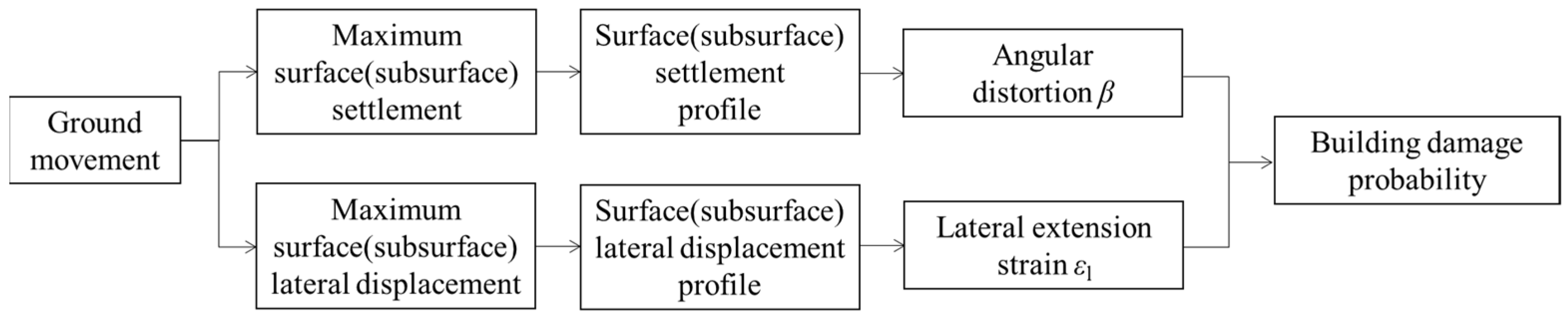
4. Assessment of Adjacent Building Damage with Ground Movements

4.1. DPI of the Building

To accurately assess the damage to adjacent buildings, the ground movement behind the excavations can be obtained by the proposed simplified evaluation. Based on the ground movement and building information, such as the location and geometry of the building, the angular distortion, β, and lateral extension strain, ε_l, can be obtained by the equations in Figure 1, and the DPI of the building can be determined using the methods proposed by Schuster et al. [30]. The level of building damage can then be assessed by interpreting the DPI results. The DPI is expressed as Equations (11)–(13) [16,30].

$$\mathrm{DPI}={\epsilon }_{\mathrm{p}}/(1/200)\times 100$$

(11)

$${\epsilon }_{\mathrm{p}}=[({\epsilon }_{\mathrm{h}}){(\cos {\theta }_{\max })}^2+\beta (\sin {\theta }_{\max })(\cos {\theta }_{\max })]$$

(12)

$${\theta }_{\max }=(1/2){\tan }^{-1}(\beta /{\epsilon }_{\mathrm{h}})$$

(13)

where ε_p is the maximum principal tensile strain, and θ_max denotes the direction of crack formation measured from the vertical plane.

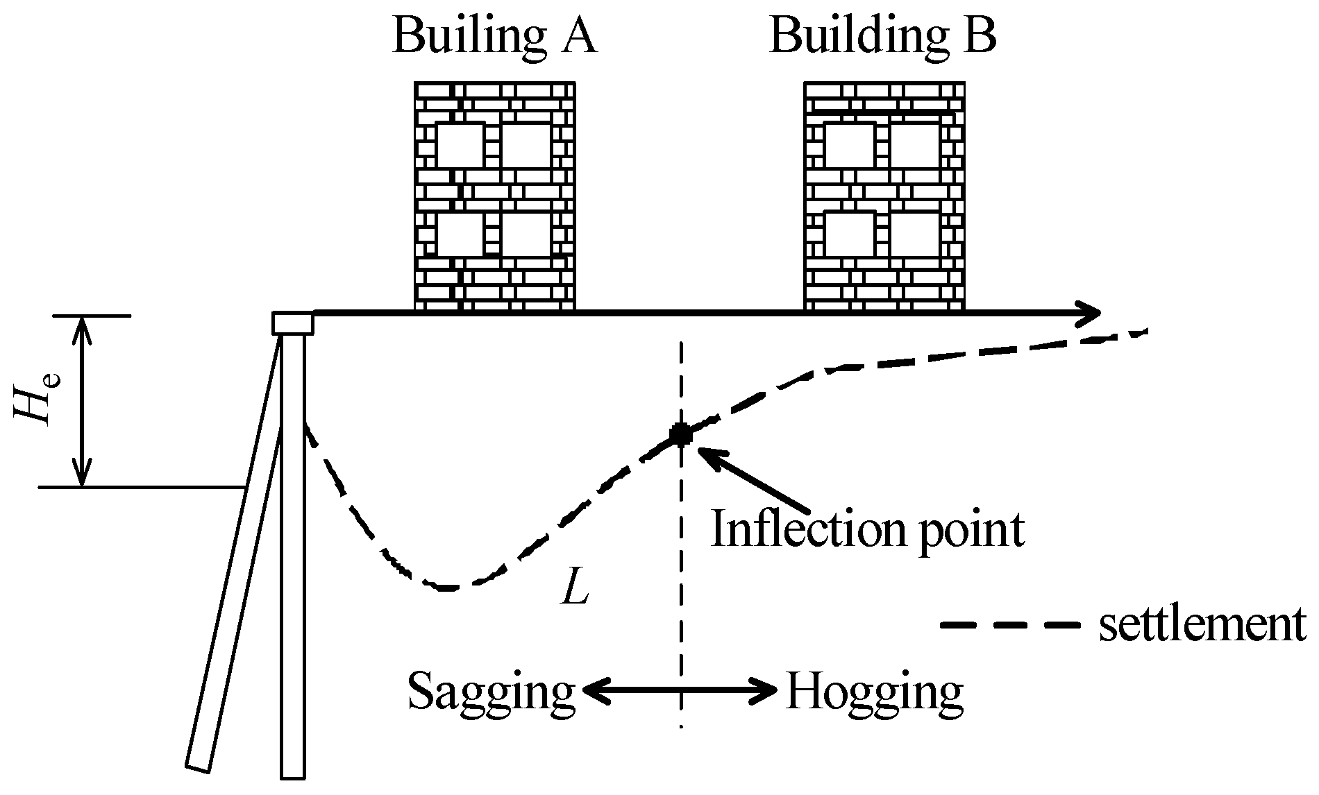
4.2. Determination of the Building Damage Pattern

The ground settlement profile behind the excavation supported by the IVFRW has a concave shape. Figure 15 illustrates that buildings at different locations from the excavation are affected by different settlement patterns. According to the inflection point of the curve, the effect of the settlement profile on building damage should be taken into account [4]. Generally, when comparing buildings with the same DPI, the damage caused by the hogging pattern is more severe than that caused by the sagging pattern. This is because, in the hogging pattern, tensile cracks develop earlier and faster in the upper part of the building [30,31].

The inflection point of the curve can be determined through the settlement profile. A large number of numerical analyses show that the distance from the inflection point to the retaining wall is 2.8 times that of the maximum settlement to the retaining wall. However, according to Equations (5) and (6), because of the difference in settlement curves at different depths behind the excavation, the position of the inflection point will change. Adjacent building damage can be assessed by the assessment criteria proposed by Schuster et al. [30].

However, for any complex process, it is essential to evaluate the uncertainty of the model. Due to this model uncertainty, the assessment of whether the building damage exceeds a specified condition cannot be “certain”. Therefore, the results of the assessment can be described with a probability.

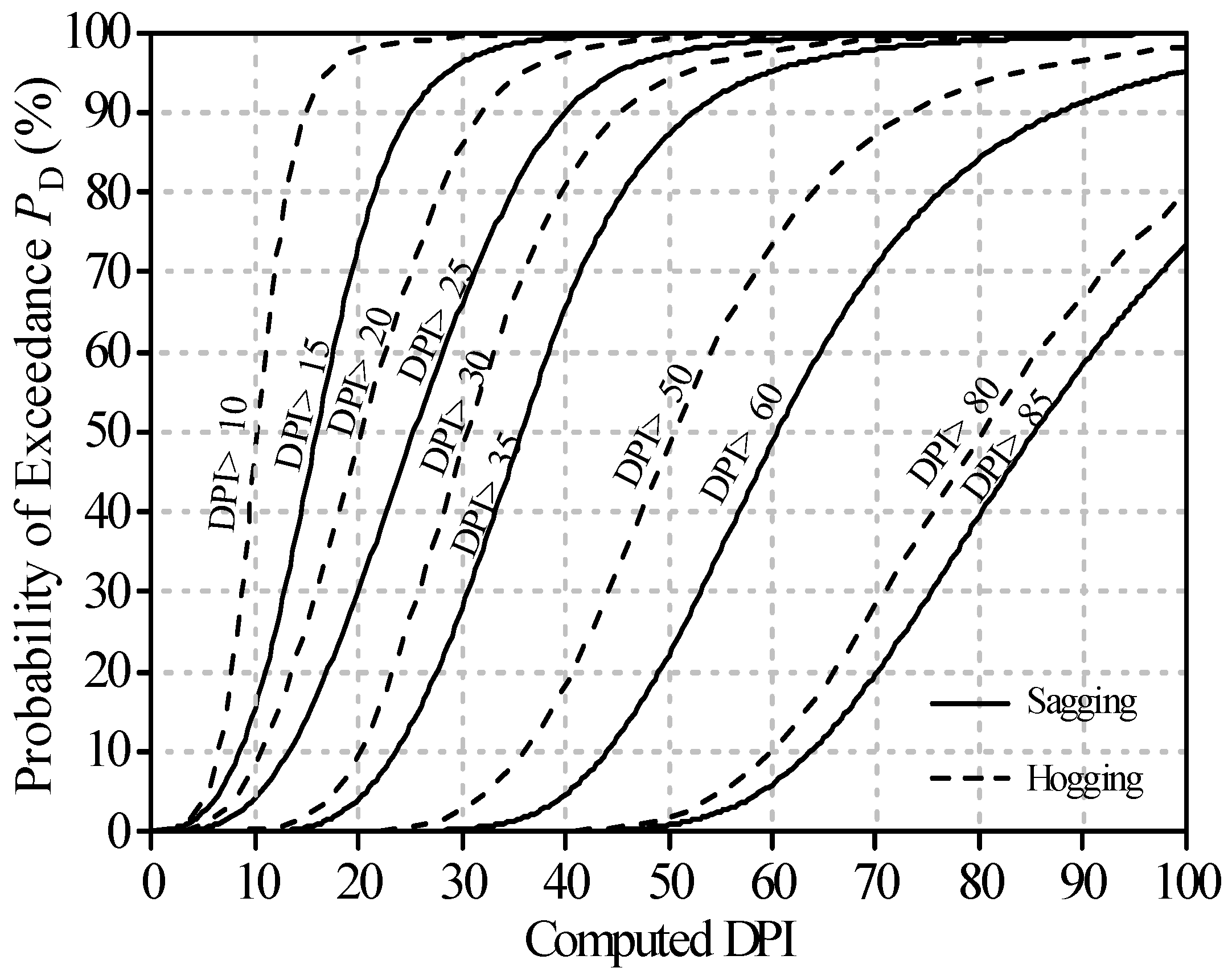
4.3. Building Damage Probability

In order to perform a probabilistic analysis, it is necessary to determine the uncertainty of the entire process for computing the DPI. By understanding the uncertainty associated with the DPI model, an engineer can estimate the probability of excavation-induced building damage. To determine the uncertainty of the DPI model, the bias factor (BF) defined in the previous section is used for analysis.

The BF is obtained by calculating the ratio of the DPI obtained from the proposed simplified calculation for ground movements in this study to the DPI obtained from the numerical analysis results. The BF is assigned a Gaussian distribution, as shown in Equation (14), and the mean (μ) and variance (σ) are 1.0 and 0.24, respectively. Given the mean and variance of the DPI for a specific case, the probability density function of the BF can be determined.

$$f(x)=\frac{1}{\sqrt{2\pi }\sigma }\exp (-\frac{{(x-\mu )}^2}{2{\sigma }^2})$$

(14)

By utilizing the probability density function of the bias factor (BF), it is possible to determine the probability of surpassing a specified DPI value. For example, the DPI obtained from the DPI model is 50, and the probability of exceeding 70 of the DPI obtained from the DPI model is the probability of exceeding 1.4 of the BF. The probability of exceeding 1.4 of BF can be determined through the probability density function of BF. To assess the probability of building damage resulting from an excavation supported by IVFRW, a simplified chart was developed, as depicted in Figure 16. The curves displayed in this chart were derived from repeated analyses of the aforementioned probability density function of BF for different deterministically computed DPI values, considering various specified damage levels.

From the user’s standpoint, the probability of sustaining building damage exceeding a specified level can be read from the chart with a calculated DPI value. For instance, if a deterministically computed DPI of 50 (sagging) is entered, the chart indicates a probability of exceeding moderate damage of 87% and a probability of exceeding severe damage of 22%.

5. Conclusions

Based on the analysis of the article, the following conclusions were drawn:

(1)

A series of numerical models for excavation supported by IVFRW were carried out in this study. Equations were proposed to predict the maximum ground settlement and lateral displacement behind excavation, using the least-squares method. The parameters needed for the equations are the excavation geometry, the soil properties (S_u/σ’_v), and the information of the retaining structure (H and θ).

(2)

A dimensionless profile of settlement was proposed, derived from the average results of numerical models. Combined with the maximum settlement value and its dimensionless profile, the settlement outside the IVFRW-retained excavation can be predicted. To validate the accuracy of the predictions, three case histories supported by IVFRW were utilized, and the results demonstrated a favorable agreement between the predictions and observations. The proposed simplified evaluation method offers a rapid and dependable assessment of ground movements caused by excavation.

(3)

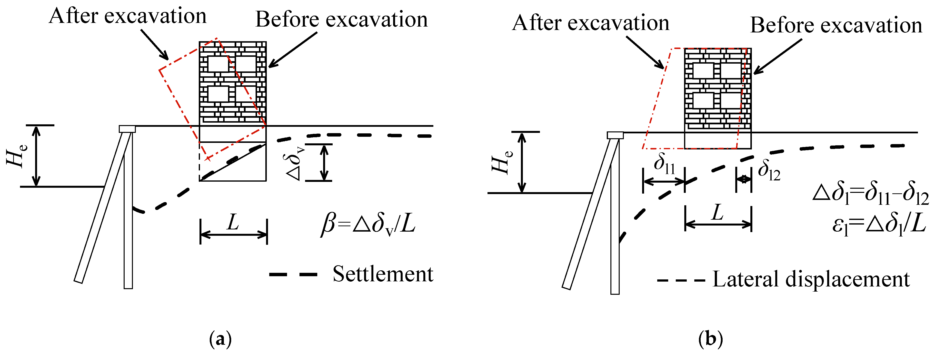
Through the prediction of soil movements, the angular distortion, β, and the lateral extension strain, ε_l, of the building can be obtained. The damage potential index of the adjacent buildings can, thus, be calculated. Based on the settlement area (sagging or hogging) of the buildings and the probability density function of the bias factor, the probability of a building outside the excavation surpassing a specified damage level can be assessed.

References

1. Peck, R.B. Deep excavations and tunneling in soft ground. In Proceedings of the 7th ICSMFE, International Conference on Soil Mechanics and Foundation Engineering, Mexico City, Mexico, 29 August 1969; Balkema: Rotterdam, The Netherlands, 1969. [Google Scholar]
2. Hsieh, P.G.; Ou, C.Y. Shape of ground surface settlement profiles caused by excavation. Can. Geotech. J. 1998, 35, 1004–1017. [Google Scholar] [CrossRef]
3. O’Rourke, T.D.; Clough, G.W. Construction induced movements of in-situ walls. In Geotechnical Special Publication: Design and Performance of Earth Retaining Structures; ASCE: Reston, VA, USA, 1990; pp. 439–470. [Google Scholar]
4. Ou, C.Y.; Teng, F.; Li, C.W. A simplified estimation of excavation-induced ground movements for adjacent building damage potential assessment. Tunn. Undergr. Space Technol. 2020, 106, 103561. [Google Scholar] [CrossRef]
5. Li, M.G.; Demeijer, O.; Chen, J.J. Effectiveness of servo struts in controlling excavation-induced wall deflection and ground settlement. Acta Geotech. 2020, 15, 2575–2590. [Google Scholar]
6. Ranasinghe, R.; Jaksa, M.; Kuo, Y.; Nejad, F.P. Application of artificial neural networks for predicting the impact of rolling dynamic compaction using dynamic cone penetrometer test results. J. Rock Mech. Geotech. Eng. 2017, 2, 150–159. [Google Scholar]
7. Mahmood, Z.; Qureshi, M.U.; Memon, Z.A.; Imran Latif, Q.B.A. Ultimate Limit State Reliability-Based Optimization of MSE Wall Considering External Stability. Sustainability 2022, 14, 4968. [Google Scholar]
8. Russo, G.; Nicotera, M.V.; Autuori, S. San Pasquale station of line 6 in Naples: Measurements and numerical analyses. Procedia Eng. 2016, 143, 1503–1510. [Google Scholar]
9. Wang, X.; Cheng, C.; Li, J.; Zhang, J.; Ma, G.; Jin, J. Automated monitoring and evaluation of highway subgrade compaction quality using artificial neural networks. Autom. Constr. 2023, 145, 104663. [Google Scholar]
10. He, Y.; Liu, Y.; Zhang, Y.; Yuan, R. Stability assessment of three-dimensional slopes with cracks. Eng. Geol. 2019, 252, 136–144. [Google Scholar]
11. Zhou, H.; Liu, X.; Tan, J.; Zhao, J.; Zheng, G. Seismic fragility evaluation of embankments on liquefiable soils and remedial countermeasures. Soil Dyn. Earthq. Eng. 2023, 164, 107631. [Google Scholar]
12. Zhou, Z.; Ding, H.; Miao, L.; Gong, C. Predictive model for the surface settlement caused by the excavation of twin tunnels. Tunn. Undergr. Space Technol. 2021, 114, 104014. [Google Scholar]
13. Kung, G.T.; Juang, C.H.; Hsiao, E.C.; Hashash, Y.M. Simplified model for wall deflection and ground-surface settlement caused by braced excavation in clays. J. Geotech. Geoenviron. Eng. 2007, 133, 731–747. [Google Scholar] [CrossRef]
14. Fan, X.-Z.; Phoon, K.-K.; Xu, C.-J.; Tang, C. Closed-form solution for excavation-induced ground settlement profile in clay. Comput. Geotech. 2021, 137, 104266. [Google Scholar]
15. Russo, G.; Nicotera, M.V. 3D Displacement Field Around a Deep Excavation. In Lecture Notes in Civil Engineering, Challenges and Innovations in Geomechanics: Proceedings of the 16th International Conference of IACMAG-Volume 2 16; Springer International Publishing: Berlin/Heidelberg, Germany, 2021; pp. 206–214. [Google Scholar]
16. Son, M.; Cording, E.J. Estimation of building damage due to excavation-induced ground movements. J. Geotech. Geoenviron. Eng. 2005, 131, 162–177. [Google Scholar] [CrossRef]
17. Zheng, G.; He, X.P.; Zhou, H.Z.; Diao, Y.; Li, Z.; Liu, X. Performance of inclined-vertical framed retaining wall for excavation in clay. Tunn. Undergr. Space Technol. 2022, 130, 104767. [Google Scholar] [CrossRef]
18. Benz, T. Small-Strain Stiffness of Soil and Its Numerical Consequences. Ph.D. Thesis, University of Stuttgart, Stuttgart, Germany, 2007. [Google Scholar]
19. Xu, D.-S.; Borana, L.; Yin, J.-H. Measurement of small strain behavior of a local soil by fiber Bragg grating-based local displacement transducers. Acta Geotech. 2014, 9, 935–943. [Google Scholar] [CrossRef]
20. Ng, C.W.W.; Hong, Y.; Soomro, M. Effects of piggyback twin tunnelling on a pile group: 3D centrifuge tests and numerical modelling. G’eotechnique 2015, 65, 38–51. [Google Scholar] [CrossRef]
21. Calvello, M.; Finno, R.J. Selecting parameters to optimize in model calibration by inverse analysis. Comput. Geotechnics 2004, 31, 410–424. [Google Scholar] [CrossRef]
22. Nie, J.; Cui, Y.; Senetakis, K.; Guo, D.; Wang, Y.; Wang, G.; Feng, P.; He, H.; Zhang, X.; Zhang, X.; et al. Predicting residual friction angle of lunar regolith based on Chang’e-5 lunar samples. Sci. Bull. 2023, 68, 730–739. [Google Scholar]
23. Karthigeyan, S.; Ramakrishna, V.; Rajagopal, K. Numerical investigation of the effect of vertical load on the lateral response of piles. J. Geotech. Geoenvironmental Eng. 2007, 133, 512–521. [Google Scholar] [CrossRef]
24. Lim, A.; Ou, C.Y.; Hsieh, P.G. Evaluation of clay constitutive models for analysis of deep excavation under undrained conditions. J. GeoEng. 2010, 5, 9–20. [Google Scholar] [CrossRef]
25. Brinkgreve, R.B.J.; Kumarswamy, S.; Swolfs, W.M. PLAXIS; Version 2015 Manual; Delft University of Technology: Delft, The Netherlands, 2015. [Google Scholar]
26. Wong, K.S.; Broms, B.B. Lateral wall deflections of braced excavations in clay. J. Geotech. Eng. 1989, 115, 853–870. [Google Scholar] [CrossRef]
27. Hsieh, P.G. Prediction of maximum ground movements induced by deep excavation in clay. J. Chin. Inst. Civ. Hydraul. Eng. 2001, 13, 489–498. [Google Scholar]
28. Zhou, H.; Shi, Y.; Yu, X.; Xu, H.; Zheng, G.; Yang, S.; He, Y. Failure mechanism and bearing capacity of rigid footings placed on top of cohesive soil slopes in spatially random soil. Int. J. Geomech. 2023, 23, 04023110. [Google Scholar]
29. Yang, S.; Leshchinsky, B.; Cui, K.; Zhang, F.; Gao, Y. Unified approach toward evaluating bearing capacity of shallow foundations near slopes. J. Geotech. Geoenviron. Eng. 2019, 145, 04019110. [Google Scholar]
30. Schuster, M.; Kung, G.T.-C.; Juang, C.H.; Hashash, Y.M.A. Simplified model for evaluating damage potential of buildings adjacent to a braced excavation. J. Geotech. Geoenviron. Eng. 2009, 135, 1823–1835. [Google Scholar] [CrossRef]
31. Burland, J.B.; Wroth, C.P. Settlement of Buildings and Associated Damage; Building Research Establishment: Liverpool, UK, 1975. [Google Scholar]
Figure 1. Schematic diagram of the angular distortion, β, and lateral extension strain, εl. (a) Schematic diagram of the angular distortion, β, calculation. (b) Schematic diagram of the lateral extension strain, εl, calculation.
Applsci 13 09485 g001
Figure 2. The project site and instrumentation layout.
Applsci 13 09485 g002
Figure 3. Profile of section E-E. Note: Unless otherwise specified, all other units are in millimeters.
Applsci 13 09485 g003
Figure 4. Illustrations of section E-E of the excavation.
Applsci 13 09485 g004
Figure 5. Comparison of wall deflection and settlement of ground surface.
Applsci 13 09485 g005
Figure 6. Numerical model of the IVFRW.
Applsci 13 09485 g006
Figure 7. Flowchart of the proposed simplified method.
Applsci 13 09485 g007
Figure 8. The relationships of the maximum surface settlement for different angles.
Applsci 13 09485 g008
Figure 9. Comparison of the computed maximum surface settlement of hypothetical cases obtained from the FEM analysis and those from the prediction model.
Applsci 13 09485 g009
Figure 10. Base function distribution diagram.
Applsci 13 09485 g010
Figure 11. Dimensionless curve of soil settlement behind the IVFRW (θ = 20°, z/He = 0.25).
Applsci 13 09485 g011
Figure 12. Dimensionless curve of soil settlement behind the IVFRW.
Applsci 13 09485 g012
Figure 13. Site plans of the projects and profiles of the studied sections: (a) Case 1, (b) Case 2, and (c) Case 3.
Applsci 13 09485 g013
Figure 14. Comparison of predictions of surface settlement profiles with field observations: (a) Case 1, (b) Case 2, and (c) Case 3.
Applsci 13 09485 g014
Figure 15. Sagging and hogging damage patterns of buildings.
Applsci 13 09485 g015
Figure 16. Simplified chart for building damage probability caused by excavation.
Applsci 13 09485 g016