Multi-Lidar System Localization and Mapping with Online Calibration

Abstract

Currently, the demand for automobiles is increasing, and daily travel is increasingly reliant on cars. However, accompanying this trend are escalating traffic safety issues. Surveys indicate that most traffic accidents stem from driver errors, both intentional and unintentional. Consequently, within the framework of vehicular intelligence, intelligent driving uses computer software to assist drivers, thereby reducing the likelihood of road safety incidents and traffic accidents. Lidar, an essential facet of perception technology, plays an important role in vehicle intelligent driving. In real-world driving scenarios, the detection range of a single laser radar is limited. Multiple laser radars can improve the detection range and point density, effectively mitigating state estimation degradation in unstructured environments. This, in turn, enhances the precision and accuracy of synchronous positioning and mapping. Nonetheless, the relationship governing pose transformation between multiple lidars is intricate. Over extended periods, perturbations arising from vibrations, temperature fluctuations, or collisions can compromise the initially converged external parameters. In view of these concerns, this paper introduces a system capable of concurrent multi-lidar positioning and mapping, as well as real-time online external parameter calibration. The method first preprocesses the original measurement data, extracts linear and planar features, and rectifies motion distortion. Subsequently, leveraging degradation factors, the convergence of the multi-lidar external parameters is detected in real time. When deterioration in external parameters is identified, the local map of the main laser radar and the feature point cloud of the auxiliary laser radar are associated to realize online calibration. This is succeeded by frame-to-frame matching according to the converged external parameters, culminating in laser odometer computation. Introducing ground constraints and loop closure detection constraints in the back-end optimization effectuates global estimated pose rectification. Concurrently, the feature point cloud is aligned with the global map, and map update is completed. Finally, experimental validation is conducted on data acquired from Chang’an University to substantiate the system’s online calibration and positioning mapping accuracy, robustness, and real-time performance.

1. Introduction

Intelligent vehicles rely on key technologies such as environmental perception, intelligent decision-making, control execution, and system design technology [1,2]. Among these, positioning technology underpins the functionalities of each module. Only with precise knowledge of the vehicle’s position and orientation in the current environment can reliable information be provided for perception and planning decisions [3,4,5]. In addition to GPS for self-driving vehicles’ positioning, two sensor types, namely lidar and cameras, are also widely used in positioning technology [6]. Compared to other sensors, lidar offers the advantages of an extended detection range, immunity to adverse weather conditions, and depth information [7,8]. Furthermore, it is prominently featured in cutting-edge research [9].

In lidar positioning, two schemes prevail: multiple lidar and single lidar [10]. Although a single multi-line lidar yields rich information, inherent blind spots may arise due to installation locations, leading to relatively sparse point cloud scans in some areas and close ranges [11,12,13]. To address these limitations, self-driving vehicles are equipped with multiple laser radars employing low scanning lines. This mitigates issues of blind spots and sparse point clouds found in single laser radars, while considering cost-effectiveness. Lidars with low scanline resolution are economically advantageous over their high scanline resolution counterparts [14,15]. Therefore, building upon the foundation of multi-lidar systems, this paper introduces a system capable of concurrent multi-lidar positioning, mapping, and real-time external parameter calibration to meet the high-precision positioning demands of unmanned vehicles.

Multi-lidar extrinsic calibration is generally categorized into two methods: reference markers and motion-based [16]. The method based on reference markers centers on point cloud registration, typically involving feature extraction for matching or minimizing spatial distances between point clouds. Bo Shi [17] and others propose using two lidars to measure structured scenes from different perspectives, conducting multiple repeated scans by altering the pose of the sensor carrier, extracting at least three pairs of planes, and forming constraints to determine external parameters. This method obviates the need for artificial calibration boards, relying solely on walls and floors. He Yanbing and Ye Bin [18] extract 3D-HARRIS key points from original point cloud data, use the histogram of orientation (SHOT) feature descriptor for characterization, and employ a random sample consensus algorithm for point cloud registration. Feature descriptors construct vectors, gauging similarity through vector subtraction and modulus. Jianhao Jiao and Qinghai Liao et al. [19] select three linearly independent corner planes, extract the corresponding plane features through the RANSAC algorithm, retain the largest three planes based on the number of feature points, match plane features and normal vectors of the two lidars, and solve the displacement vector via the least squares method along with the rotation matrix through the Kabsch algorithm [20]. Following the acquisition of the initial external parameters, a nonlinear optimization model is established and iterated until convergence, yielding precise extrinsic results. In natural environments, dedicated reference markers for calibration are often elusive, necessitating motion-based calibration.

The motion-based method: Livox introduces a target-free calibration algorithm that assumes consistency among local 3D models scanned by multiple lidars then reconstructs the point cloud from both auxiliary and main lidars during movement [21,22,23]. These maps are registered until the algorithm converges. Xiyuan Liu and FuZhang [24] propose generating common visible features by overlapping common-view fields of view through motion, facilitating mapping and registration of all lidars to acquire reference radar pose and point cloud maps for all radars. Jiao et al. [25] achieve automatic online calibration of radar pose using the multi-lidar odometer based on the sliding window approach. They determine relative motion between two lidar frames through line and surface feature frame matching, enabling calculation of initial states for each radar’s coordinate system pose. The hand–eye calibration problem is then employed to complete coarse external parameter calibration. The initial outcomes of the algorithm’s rough external parameter calibration serve as the foundation for constructing an optimization problem. By associating and matching the feature point cloud within the sliding window with the reference radar’s local map, accurate calibration results are attained through continuous iterations until convergence.

Current research calls for enhancements in efficiency and accuracy. Many multi-sensor, external parameter calibration strategies are carried out offline and often in a controlled calibration environment. Prolonged driving can lead to shifts in sensor position and orientation, rendering prior offline calibration outcomes invalid and affecting the usability of autonomous driving functions. The online calibration of external parameters among multiple lidars within a varying environment also bears significant research importance.

The innovation aspects of this paper are outlined as follows:

(1)

The registration method based on line and surface features is used for point cloud matching, and the LM algorithm is used for nonlinear optimization. A refined root mean square error (RMSE) method is introduced to evaluate the point cloud registration accuracy.

(2)

A feature fusion strategy, grounded in feature point cloud smoothness and distribution, enables frame-to-frame matching using the Ceres library and LM nonlinear optimization method. This prevents an excessive number of multi-lidar feature point clouds from impairing the real-time performance of the system.

(3)

The GTSAM library is employed to formulate a graph optimization model, supplemented by a loop closure detection constraint factor grounded in the Scan Context descriptor and a ground constraint factor relying on plane feature matching. These elements collectively achieve global trajectory optimization and z-axis error limitation.

(4)

A real vehicle experimental platform is established to validate the robustness, real-time performance, and accuracy of the online calibration algorithm presented in this paper. This study also verifies that the multi-radar SLAM system has a more pronounced accuracy improvement than the single radar system.

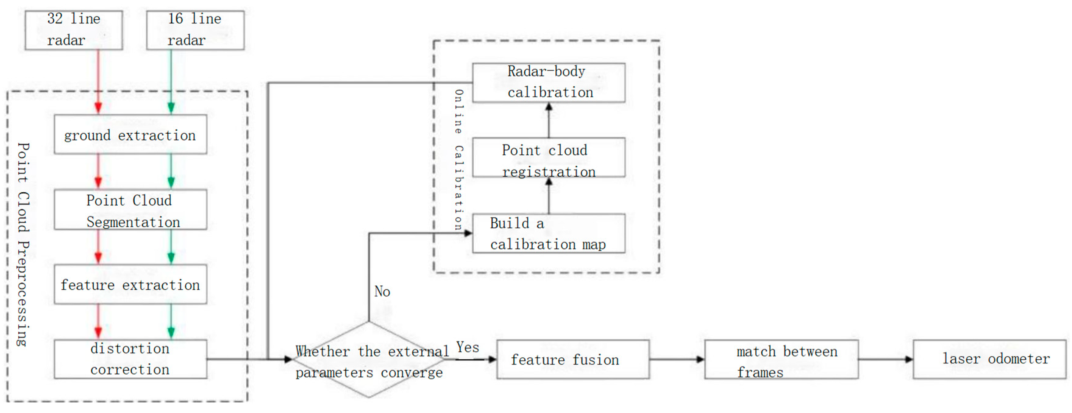
2. Front-End Laser Odometry and Online Calibration

In this paper, the point cloud data from two laser radars undergo preprocessing and feature extraction, enabling real-time calibration of external parameters among multiple laser radars. When non-convergence of external parameters is detected, the feature point cloud from the main lidar is utilized for inter-frame matching to solve the laser odometer information [26,27,28]. Concurrently, online calibration is performed to unify the coordinate systems across multiple radars and vehicles. Upon detecting the convergence of external parameters, a fusion strategy proposed in this paper is employed, merging feature point clouds from the two radars to solve the laser odometer. The specific process is illustrated in Figure 1.

2.1. Point Cloud Preprocessing

Ground point cloud screening, as depicted in Figure 2, involves two points, A and B, scanned by two adjacent laser beams on the same column. In the figure, h indicates the height difference between the points, d is the horizontal distance, and θ represents the angle between the straight line formed by the points and the horizontal plane. The determination of whether points A and B belong to the ground point cloud hinges on comparing the horizontal angle with a predetermined threshold. If it surpasses the threshold, both points are considered non-ground. Otherwise, both points are considered as part of the ground point cloud.

The angle θ can be computed as follows:

$$\theta =\arctan \left(\frac{\left|z_1-z_2\right|}{\sqrt{{\left(x_1-x_2\right)}^2+{\left(y_1-y_2\right)}^2}}\right)$$

(1)

When clustering the point cloud, the initial step involves traversing each point for processing. If the current point has not been marked, it is designated as a new cluster, and the current point is then used as a center for traversal of its four neighbors: up, down, left, and right. During this process, it is essential to calculate the angle between the laser radar, the current point, and the neighbor point. Should the angle exceed the designated threshold, both the current point and the neighbor point are categorized under the same point cloud. The calculation process is illustrated in Figure 3, where O represents the center point of the lidar, A is the current point of traversal, B denotes the neighbor of the current point, d1 is the length of line segment OA, d2 is the length of line segment OB, α is the angle between OA and OB, and θ is the angle to be calculated.

The angle θ can be computed as follows:

$$\theta =\arctan \left(\frac{d_2\ast \sin \alpha }{d_1-d_2\ast \cos \alpha }\right)$$

(2)

Neighbor points are continuously traversed until the current cluster no longer contains points that meet the requirements. At that point, the clustering process is deemed completed. The decision on whether to retain the cluster is based on the number of point clouds within it. If this count falls below a certain threshold, the cluster is considered invalid.

In the process of correcting point cloud motion distortion, assuming constant lidar movement speed between two frames, the prediction of relative motion between the current frames hinges on the calculation results of the laser odometer from the preceding two frames, as expressed in the following equation:

$${\left(T_{k-1}^w\right)}^{-1}{T}_k^w={\left(T_{k-2}^w\right)}^{-1}{T}_{k-1}^w$$

(3)

where $T_k^w$, $T_{k-1}^w$, and $T_{k-2}^w$ represent the laser odometer information for frames k, k − 1, and k − 2, respectively, in the world coordinate system. In accordance with the assumption of a uniform motion model, the relative motion between frames k − 2 and k − 1 is consistent with the relative motion between frames k − 1 and k. Consequently, the pose transformation for frame k can be computed. This approach effectively achieves motion distortion correction for the lidar point cloud.

2.2. Realization of Multi-Lidar Online Calibration

2.2.1. Online External Parameter Calibration

In the process of multi-lidar calibration, point clouds in different coordinate systems are brought into alignment within a common coordinate system through point cloud registration [29,30,31,32]. The assessment of point cloud registration accuracy generally employs RMSE as a quantitative metric that establishes corresponding points between two point clouds using a Kd-tree, subsequently determining the discrepancy between the Euclidean distance and the actual distance:

$$\mathrm{RMSE}=\sqrt{\frac{\sum _{i=1}^n{\left(x_i-{\widehat{x}}_i\right)}^2}{n}}$$

(4)

where n is the number of corresponding points, $x_i$ is the actual Euclidean distance between corresponding points, and ${\widehat{x}}_i$ is the Euclidean distance between corresponding points after registration. As inferred from the formula, a smaller RMSE indicates a lesser gap between the Euclidean distance and the actual distance of corresponding points after registration, signifying a higher degree of point cloud overlap. An RMSE of 0 implies complete coincidence of the two point clouds.

However, this evaluation method holds certain shortcomings. Poor point cloud registration results may yield a small number of associated corresponding points and erroneous associations, thereby affecting the reliability of calculated results [33,34]. Therefore, this paper proposes an improved RMSE index to evaluate point cloud registration accuracy. This improved index considers the number of corresponding points as a weight: the greater the count, the more dependable the index outcome, as expressed in the following:

$$\mathrm{RMSE}=\frac{1}{n^2}\sqrt{\frac{{\displaystyle \sum _{i=1}^n}{\left(x_i-{\widehat{x}}_i\right)}^2}{n}}\times {10}^6$$

(5)

During multi-lidar online external parameter calibration, the process begins by projecting the feature point cloud of the auxiliary laser radar onto the main laser radar’s coordinate system using the current external parameters, as indicated in the following:

$${\tilde{X}}_{k+1,i}^L=R{X}_{k+1,i}^L+t=G\left(X_{k+1,i}^L,T_{k+1}^L\right)$$

(6)

Within two-dimensional space, the modulus length of the cross product of two vectors equates to the area of the parallelogram formed by these vectors. Dividing the area of the parallelogram by the side length yields the distance from point i to line j_l, thus obtaining the line feature optimization equation:

$$d_e=\frac{\mid \left(X_{(k+1,i)}^L-X_{(k,j)}^L\right)\times \left(X_{(k+1,i)}^L-X_{(k,l)}^L\right)\mid }{\left|X_{(k,j)}^L-X_{(k,l)}^L\right|}$$

(7)

In three-dimensional space, the volume of a three-dimensional object can be obtained through vector dot multiplication. Similarly, the distance between point i and plane j_lm is deducible by dividing the volume by the area of the bottom surface, resulting in the optimization equation for surface characteristics:

$$d_h=\frac{\left|\left(X_{(k+1,i)}-X_{(k,j)}\right)\cdot \left(\left(X_{(k,j)}-X_{(k,l)}\right)\times \left(X_{(k,j)}-X_{(k,m)}\right)\right)\right|}{\left|\left(X_{(k,j)}-X_{(k,l)}\right)\times \left(X_{(k,j)}-X_{(k,m)}\right)\right|}$$

(8)

Based on (7) and (8), the residual equation for feature association can be unified as follows:

$$\mathrm{loss}=\sum _{i=1}^{N_e}{d}_{ei}+\sum _{i=1}^{N_h}{d}_{hi}=D\left({\tilde{X}}_{k+1,i}^L\right)$$

(9)

The total loss function can be obtained by combining (6) and (9):

$$d=F\left({\tilde{X}}_{k+1,i}^L,T_{k+1}^L\right)=D\left(G\left({\tilde{X}}_{k+1,i}^L,T_{k+1}^L\right)\right)$$

(10)

Substituting into (11), we evaluate as follows:

$$\mathsf{\Delta }T=-{\left(J{J}^T+\lambda D^{T}D\right)}^{-1}{J}^{T}d$$

(11)

The gradient descent is then applied using the following equation:

$$T_{k+1}^L\leftarrow T_{k+1}^L-{\left(J{J}^T+\lambda D^{T}D\right)}^{-1}{J}^{T}d$$

(12)

Ultimately, the refined pose transformation matrix serves as an accurate extrinsic parameter matrix used to transform the feature point cloud of the auxiliary lidar, thereby yielding the calibration result.

2.2.2. Convergence Assessment of External Parameters

The LM algorithm used in this paper transforms the nonlinear problem into a local linear problem by computing the Jacobian matrix J of the error function. Consequently, the linear problem of each row can be regarded as a hyperplane of the solution space. The resultant solution x is a point in this space, fulfilling the requirement of minimal Euclidean distance to every hyperplane. The degeneracy factor is established by investigating the geometric distribution of the plane, incorporating additional hyperplane constraints and perturbations, as shown in Figure 4.

In Figure 4, the black line represents the plane constraint, the orange line denotes the additional hyperplane constraint, the blue point x₀ represents the optimization problem’s solution, c is the normal vector of the additional hyperplane constraint with a modulus length of 1, δd denotes the offset distance of the hyperplane after adding the disturbance, and δx_c is the offset distance of the constraint, i.e., the offset distance of x₀ after adding the disturbance. The derivation of the degradation factor can be obtained. Since the constraint intersects with x₀, the latter is not altered by the additional constraint, resulting in the following equation:

$$c^T\left(x-x_0\right)=0,\parallel c\parallel =1$$

(13)

If the constraint is moved along its normal direction c by a certain distance, then x₀ will produce a displacement of δx_c in the same direction. For a given disturbance, let δx_c* represent the maximum displacement:

$$\delta x_c^{\ast }=\underset{c}{\max }\delta x_c$$

(14)

The definition of the degradation factor is then expressed as follows:

$$D=\frac{\delta d}{\delta x_c{}^{\ast }}$$

(15)

Namely, the degradation factor is defined as the ratio of the hyperplane’s movement distance to the solution’s maximum displacement. Evidently, a smaller value implies greater system stability. Simultaneously considering (14) and (15), we obtain the following:

$$\left[\begin{array}{c}A\\ c^T\end{array}\right]x=\left[\begin{array}{c}b\\ c^T{x}_0\end{array}\right]$$

(16)

After introducing perturbations, we have the following:

$$\left[\begin{array}{c}A\\ c^T\end{array}\right]x=\left[\begin{array}{c}b\\ c^T{x}_0+\delta d\end{array}\right]$$

(17)

Substituting the left pseudo-inverse ${\left[\begin{array}{c}A\\ c^T\end{array}\right]}_{left}^{-1}={\left(\left[\begin{array}{c}\begin{array}{cc}{A}^T& c\end{array}\end{array}\right]\left[\begin{array}{c}A\\ c^T\end{array}\right]\right)}^{-1}\left[\begin{array}{c}\begin{array}{cc}{A}^T& c\end{array}\end{array}\right]$ into (16), we obtain the following:

$$\delta x={\left(A^{T}A+c{c}^T\right)}^{-1}c\delta d$$

(18)

The displacement δx_c in the c direction can be calculated as the dot product of c and δx:

$$\delta x_c=c^T\delta x=c^T{\left(A^{T}A+c{c}^T\right)}^{-1}c\delta d$$

(19)

This illustrates that the degradation factor only relates to the original constraint direction A, independent of the initial constraint position b; parallel original constraint directions induce degradation.

Converting $c$ and $c^T$ according to the pseudo-inverse $c_{left}^{-1}={\left(c^{T}c\right)}^{-1}{c}^T=c^T$, $c_{right}^{-1}=c{\left(c^{T}c\right)}^{-1}=c$ yields the following:

$$\delta x_c={\left(c^T{A}^{T}Ac+1\right)}^{-1}\delta d$$

(20)

For maximizing, (21) must be satisfied:

$$\begin{array}{l}{c}^{\ast }=\arg \underset{c}{\min }{c}^T{A}^{T}Ac\\ \parallel c\parallel =1.\end{array}$$

(21)

Since the modulus of c is 1, (21) can also be expressed as follows:

$$c^{\ast }=\arg \underset{c}{\min }\frac{c^T{A}^{T}Ac}{c^{T}c}$$

(22)

which takes the form of a Rayleigh quotient, with the minimum value occurring when c is the minimum eigenvalue of A^TA. Introducing c here, we have the following:

$$\delta x_c^{\ast }=\frac{\delta d}{{\lambda }_{\min }+1}$$

(23)

Thus, the degradation factor is obtained as follows:

$$D={\lambda }_{\min }+1$$

(24)

In summary, the magnitude of the degradation factor allows for judgment regarding degradation within the constraint. The information matrix’s minimum eigenvalue exhibits a positive linear correlation with the degradation factor, which reveals the condition of the optimization-based state estimation problem, enabling assessment of whether sufficient constraints exist within the online calibration optimization problem to solve the precise external parameters. In this paper, the information matrix is defined based on the computed Jacobian matrix J, and convergence of multi-lidar external parameters is evaluated by comparing the minimum eigenvalue of the information matrix to a designated threshold.

2.3. Inter-Frame Registration

After obtaining the feature point clouds of two consecutive frames, they are connected through scan-to-scan. The Ceres library is used to solve the least squares problem. Its definition is formulated as follows:

$$\begin{array}{l}\underset{x}{\min }\frac{1}{2}{\displaystyle \sum _i}{\rho }_i\left(‖f_i{\left(x_{i1},\cdots ,x_{in}\right)}^2‖\right)\\ \mathrm{s}.\mathrm{t}. l_j\le x_j\le u_j\end{array}$$

(25)

where ${\rho }_i\left(‖f_i{\left(x_{i1},\cdots ,x_{in}\right)}^2‖\right)$ is the residual block functioning as the cost function and depending on the parameter block $\left[x_{i1},x_{i2}\cdots ,x_{in}\right]$, while l_j and u_j are the upper and lower limits of the j-th optimization variable, respectively. Typically, these boundaries do not restrict the optimization variable’s range; $l_j=-\infty$, $u_j=\infty$. Additionally, the loss function ${\rho }_i=x$ is assumed to be an identity function. The objective function is the sum of squares of multiple terms, resulting in an unconstrained nonlinear least squares formulation:

$$\frac{1}{2}\sum _i{f}_i{\left(x_{i1},x_{i2}\cdots ,x_{in}\right)}^2$$

(26)

3. Back-end Optimization and Map Construction

The back-end optimization in this study is based on the graph optimization library GTSAM. The global pose is optimized by constructing a pose graph supplemented with loopback and ground constraint factors. Additionally, key frames are extracted, and their feature point clouds are matched to the global map for comprehensive map generation and updating.

3.1. Loop Detection Based on Scan Context

In this study, the Scan Context environment descriptor is selected. The initial step involves reorganizing the point cloud using a ring and sector methodology. This procedure maps the 3D point cloud into a 2D feature map, as illustrated in Figure 5.

By segmenting the point cloud into rings and using a small sector for finer division, distinct indexed regions can be located within the two-dimensional feature map. The feature map’s values correspond to the highest reflection point’s elevation in the respective area. This approach extracts a two-dimensional feature map while retaining the spatial structural characteristics of the point cloud, as exemplified in Figure 6.

Upon extracting the Scan Context descriptor, defining a distance calculation formula is necessary to assess the similarity between two descriptors. Given the Scan Context of two point clouds, denoted as I^q and I^c, the cosine distance of the column vectors in the two feature matrices is used as the distance measure, and the result is then normalized by division as expressed in the following:

$$d\left(I^q,I^c\right)=\frac{1}{N}\sum _{i=1}^N\left(1-\frac{c_j^q{c}_j^c}{c_j^q{c}_j^c}\right)$$

(27)

Directly computing the distance of column vectors is inadequate when dealing with scenarios involving perspective switches within the same scene. Consequently, it is crucial to calculate the distance between all column vectors of the two Scan Contexts, selecting the minimum value as the final distance.

To ensure efficient searching and real-time performance of the SLAM system, sparse optimization is also necessary. Introducing the concept of the ring key facilitates obtaining a descriptor insensitive to rotation from the column vector in the Scan Context descriptor:

$$\psi \left(r_i\right)=\frac{r_i{}_0}{N}$$

(28)

Given that ring characteristics are unaffected by the vehicle’s orientation, the ring key becomes rotation insensitive. While it contains less information compared to the complete Scan Context descriptor, it enhances candidate frame searching efficiency. By constructing a Kd-tree and selecting the Scan Context corresponding to the multiple historical ring keys most similar to the ring key of the current scene, the nearest scene can be identified using the distance calculation formula described in the preceding section. This entire scene recognition process is depicted in Figure 7.

3.2. Z-Axis Error Limitation Based on Ground Constraints

As the vehicle’s travel distance increases, the cumulative error of the z-axis also progressively increases, as indicated by the following:

$${ \mathrm{error}}_z=S\times \sin \varphi$$

(29)

where S is the actual travel distance of the vehicle and $\varphi$ is the pitch angle.

This paper adopts a constraint to extend the planar point cloud feature into a ground to mitigate the drift issue of the z-axis.

The fitted global ground equation is first initialized:

$$A_{w}x+B_{w}y+C_{w}z+D_w=0$$

(30)

RANSAC fitting is concurrently applied to the current frame’s ground point cloud to obtain the ground equation:

$$A_{i}x+B_{i}y+C_{i}z+D_i=0$$

(31)

Since the two plane equations are in different coordinate systems, it becomes essential to project the global plane equation PW from the world coordinate system to the radar coordinate system of the current frame i, as expressed in the following equation:

$$P_w^{\prime }=T_i^w{P}_w$$

(32)

Upon obtaining the two plane equations that share a unified coordinate system, the transformation relationship between the two normal vectors comes into play for constructing the residual, as illustrated in Figure 8.

Considering the two angles in Figure 8, the normal vectors of the two planes can be made entirely consistent. Subsequently, the intersection point of the two planes is measured to formulate the residual in three dimensions as follows:

$$\alpha =\arctan \left(\frac{y}{x}\right)$$

(33)

$$\beta =\arctan \left(\frac{z}{\sqrt{y^2+x^2}}\right)$$

(34)

$${ \mathrm{error}}_d=\left|D_w-D_i\right|$$

(35)

These residual items in all three dimensions are integrated into the least squares problem. Through this process, optimization is conducted collectively with other constraints.

3.3. Map Construction and Update

The map construction in the laser SLAM system outlined in this paper involves registering the feature point cloud of each key frame onto the global map. In comparison to the inter-frame matching of the odometer, this approach boasts higher matching accuracy; however, it is accompanied by a decrease in matching speed. With the continuous expansion of the map, the computational resources required rise significantly. Therefore, the use of key frames, local map construction, and point cloud downsampling is employed to bolster scan-to-map matching speed and prevent excessive computational burden on the overall system performance.

The subsequent step entails the construction and update of the point cloud global map. The specific process is illustrated in Figure 9, where $Q_k$ represents the map point cloud constructed at time k, $Q_k$ is the feature point cloud at time k + 1, $T_k^W$ is the pose estimation of the vehicle relative to the global coordinate system at time k, and $T_{k+1}^L$ is the pose estimation of the laser odometer at time k + 1.

Consequently, the pose estimation of the vehicle relative to the global coordinate system at time k + 1 is expressed as follows:

$$T_{k+1}^W=T_{k+1}^L{T}_k^W$$

(36)

Based on the pose transformation relationship, the feature point cloud of the current frame can be projected into the global coordinate system, as expressed in the following equation:

$$P_{k+1}=T_{k+1}^W{\overline{Q}}_{k+1}$$

(37)

4. Real-World Experiment Validation and Result Analysis

4.1. Online Calibration Experiment Results and Analysis

The online calibration experiment conducted in this paper is divided into two parts. The first part verifies the robustness of the calibration algorithm by altering the installation layout of multiple laser radars. The online calibration results are then compared with actual measurements within the same scene. The second part uses diverse calibration algorithms on the same data, comparing the results of this paper’s algorithm with others to validate its accuracy and real-time efficacy.

4.1.1. Comparison and Analysis of Online Calibration Results for Different

Lidar Layouts

This section employs six multi-radar layouts, deriving actual inter-radar external parameters through manual measurements. Multiple individuals participated in the measurements, and the mean of all measurements was taken as the ultimate value, aiming to minimize manual measurement errors. The online calibration results and corresponding radar layouts are shown in

Table 1. Online calibration results for different lidar layouts.

	X (m)	Y (m)	Z (m)	Roll (°)	Pitch (°)	Yaw (°)
The 32-line lidar is placed at the center of the roof, while the 16-line lidar is placed at the center of the front of the vehicle.
Actual measurement values	0.82	0	−0.05	0	15	5
Algorithm calibration values	0.848785	−0.0669597	−0.110832	−1.01514	15.052825	4.54818
The 32-line lidar is centered on the roof, and the 16-line lidar is centered on the front of the vehicle.
Actual measurement values	0.82	0.45	−0.05	−2	15	5
Algorithm calibration values	0.788523	0.450865	−0.0857012	−2.90022	15.0670923	4.27292
The 32-line lidar is placed at the center of the roof, and the 16-line lidar is placed at the left side of the rear end.
Actual measurement values	−0.63	0.45	−0.03	1	−1	−1
Algorithm calibration values	−0.69039	0.440672	−0.010485	0.38109943	−0.78497562	−1.66093791
The 32-line lidar is mounted on the center of the roof, and the 16-line lidar is mounted on the front right of the vehicle.
Actual measurement values	0.82	−0.45	−0.05	8	15	−10
Algorithm calibration values	0.812278	−0.428665	−0.0959522	7.30276	16.0154646	−9.31442
The 32-line Lidar is placed on the roof in the center, while the 16-line Lidar is placed on the rear of the car and to the right.
Actual measurement values	−0.63	−0.45	−0.03	10	−3	−10
Algorithm calibration values	−0.644347	−0.37646	−0.078509	10.6063	−3.16483	−11.497818
The 32-line lidar is mounted on the right side of the roof, and the 16-line lidar is mounted on the left side of the roof.
Actual measurement values	0	0.67	−0.02	0	0	0
Algorithm calibration values	0.0617705	0.732039	−0.0673341	0.39993226	−0.10664561	1.47808788

.

Upon reviewing Table 1, it is evident that the online calibration outcomes closely align with actual measurements, affirming the efficacy of the calibration algorithm. Further analysis will be conducted to statistically assess deviations between the online calibration results and actual measurements, as shown in

Table 2. Deviation statistics between calibration and actual measurements for six multi-radar layout algorithms.

	X (m)	Y (m)	Z (m)	Roll (°)	Pitch (°)	Yaw (°)
maximum deviation	0.0617705	0.07364	0.060832	1.01514	1.0154646	1.497818
minimum deviation	0.007722	0.000865	0.019515	0.3993226	0.052825	0.45182
mean deviation	0.0340818	0.03901111	0.0429739	0.7062888	0.27031365	0.9168873

.

Upon analyzing Table 2, it is deduced that the maximum translation error of the online calibration algorithm is 0.0617705 m, and the maximum rotation error is 1.497818°, both falling within acceptable limits. The smaller deviation in translation calibration results can be attributed to the precision of actual translation measurements as well as minimal translation deviation between the two lidars, rendering this paper’s algorithm more capable of achieving accurate calibration results. Notably, the yaw angle exhibits greater deviation among the three rotation angles, primarily due to the lidar’s relatively low vertical resolution and limited vertical direction constraints.

4.1.2. Comparison and Analysis of Online Calibration Algorithm Results for

Multiple Lidars

In the experiment, the proposed calibration algorithm was compared with multi_lidar_calibrator [35] and OpenCalib [36]. The data collected within the same scene were used for calibration using each algorithm. Calibration results were then analyzed to discern the strengths and weaknesses of the proposed algorithm within natural scenes. The results of the three calibration algorithms are shown in Figure 10.

Visual assessment of the calibration outcomes unveils varying degrees of ineffectiveness in the other two calibration algorithms, and the proposed algorithm exhibits superior efficacy. By employing the improved RMSE method as described in this paper, along with the visualization results, calibration results from each algorithm are analyzed and compared to assess calibration quality. Statistical results are presented in

Table 3. Detailed evaluation indicators for various multi-lidar calibration algorithms.

Algorithm Name	Improved RMSE	Original RMSE	Visual Evaluation	Running Time	Corresponding Point Number
multi_lidar_calibrator	2.194913	5.33469	Poor	14,121 ms	1559
OpenCalib	1.985486	8.4994	Good	5366.5 ms	2069
my_calibration	0.914785	13.307	Excellent	98 ms	3814

.

Through detailed analysis of experimental data, it can be concluded that the calibration algorithm proposed in this paper not only guarantees the point cloud registration accuracy, but also takes into account real-time performance, ensuring that when the lidar point cloud data is input at a frequency of 10 Hz, it can be processed in a timely manner, while the other two calibration algorithms have poor real-time performance and can only be used as offline calibration algorithms. At the same time, it can be clearly seen from the visualization calibration results that the point cloud calibrated by the multi_lidar_calibrator algorithm is not well registered, but its original RMSE indicator is the smallest, which means it has the highest accuracy. The improved RMSE indicator is consistent with the visualized results, verifying the feasibility of evaluating point cloud registration based on the improved RMSE algorithm. A comprehensive analysis of experimental data underscores that the proposed calibration algorithm not only ensures accurate point cloud registration, but also balances real-time performance. It guarantees that when the lidar point cloud data is input at a frequency of 10 Hz, it can be processed promptly. Conversely, the real-time performance of the other two calibration algorithms is less satisfactory, relegating them to offline calibration use. Visual calibration results further highlight that point clouds calibrated by the multi_lidar_calibrator algorithm exhibit misalignment. However, the algorithm yields the smallest original RMSE index, indicating the highest accuracy. Notably, the improved RMSE index is consistent with the visual results, substantiating the feasibility of the point cloud registration based on the enhanced RMSE algorithm.

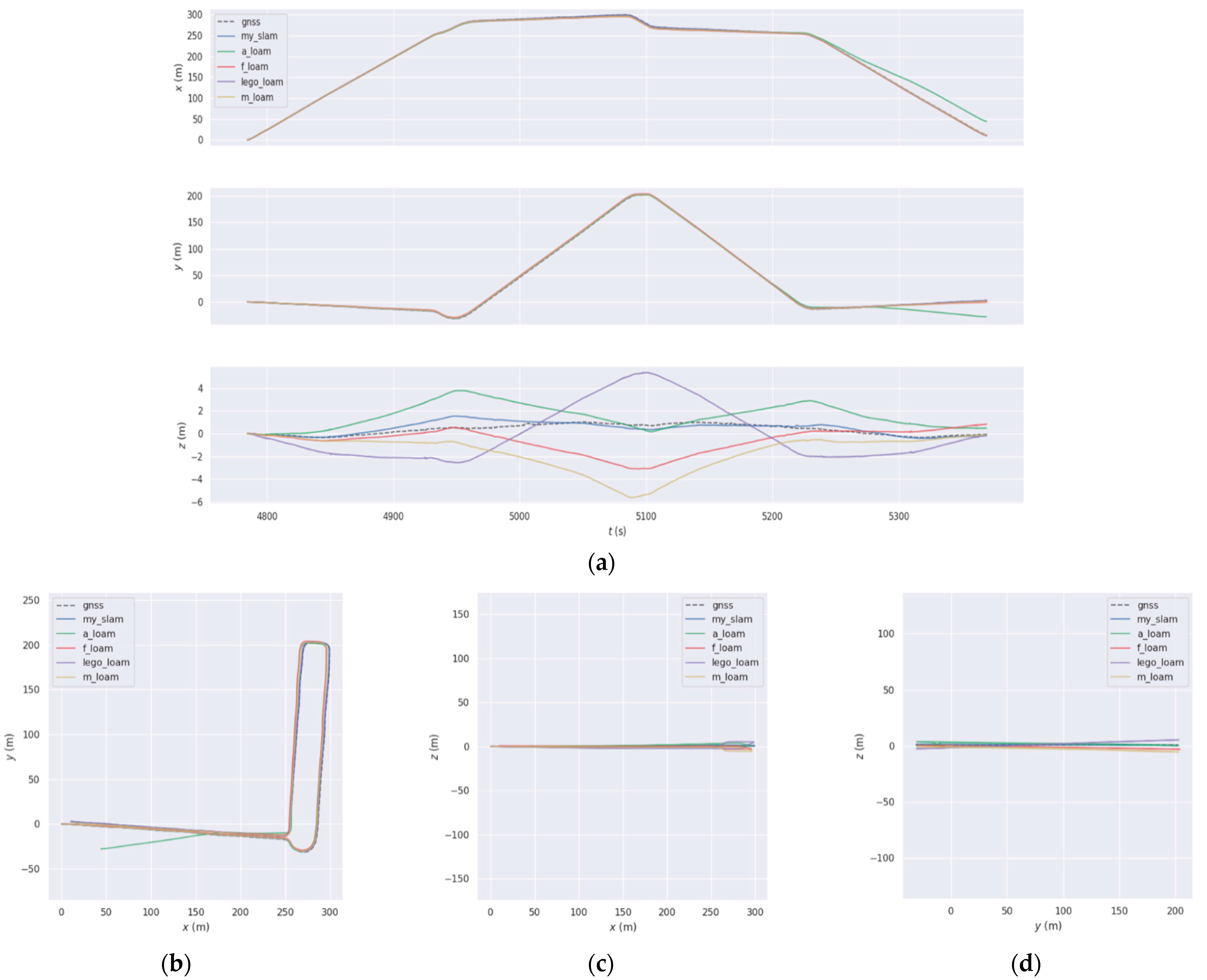
4.2. Experimental Results and Analysis of LiDAR SLAM on a Real Vehicle

In this section, the proposed SLAM algorithm is compared with other LiDAR SLAM algorithms, and the absolute pose error (APE) is obtained by comparing the estimated trajectory of the SLAM algorithm with the GPS trajectory using the EVO tool, in order to verify the accuracy of the proposed SLAM algorithm. The trajectory comparison is shown in Figure 11. The experiment in this section involves a comparison between the proposed SLAM algorithm and prominent laser SLAM algorithms. The analysis is conducted using the EVO tool. The absolute pose error (APE) is obtained by comparing the GPS trajectory with the trajectory estimated by the SLAM algorithm to validate the accuracy of the SLAM algorithm proposed in this paper. This trajectory comparison is illustrated in Figure 11.

Based on the preceding analysis, it becomes evident that, apart from the A-LOAM algorithm, the errors along the x and y axes of the other laser SLAM algorithms are relatively small. However, as historical feature points gradually vanish, the A-LOAM algorithm’s absence of loop detection renders it unsuitable for large-scale scene mapping. In the z-axis direction, all algorithms exhibit notable errors; LeGO-LOAM and M-LOAM manifest the most substantial deviations. In contrast, the SLAM algorithm presented in this paper effectively curtails z-axis errors by incorporating ground constraints, leading to the smallest error among the surveyed laser SLAM algorithms.

The APE and RPE outcomes output by the EVO tool underscore the APE values for each laser SLAM algorithm.

Table 4. APE values of different laser SLAM algorithms.

	Max (m)	Mean (m)	Median (m)	Min (m)	RMSE (m)	Std (m)
A-LOAM	44.507192	5.494679	2.910864	0.016384	10.944484	9.465212
F-LOAM	6.335769	2.797792	2.316942	0.024018	3.206701	1.566937
LeGO-LOAM	5.727396	3.054158	3.192376	0.061186	3.252286	1.117804
M-LOAM	7.572633	2.675861	1.500130	0.061675	3.459226	2.192261
My-SLAM	3.250923	2.196747	2.648033	0.028497	2.433783	1.047665

quantifies the conformity between the estimated and actual trajectories by evaluating absolute pose estimation.

These APE statistical data provide a tangible insight into the positioning accuracy of each SLAM algorithm. Using the mean average APE output as a benchmark, the algorithm outlined in this paper emerges as the most adept in trajectory estimation, due to the integration of constraints that heighten the accuracy potential of the laser SLAM system.

RPE pertains to the comparison of relative pose errors across different trajectories through attitude increments. It involves an ongoing juxtaposition between real and estimated trajectories, culminating in a localized trajectory accuracy assessment and a gauge of the SLAM system’s drift. This paper considers both rotational and translational errors. Figure 12 and

Table 5. RPE values for different laser SLAM algorithms.

	Max (m)	Mean (m)	Median (m)	Min (m)	RMSE (m)	Std (m)
A-LOAM	2.852986	0.488630	0.446949	0.002057	0.610143	0.365397
F-LOAM	2.802553	0.455393	0.426244	0.001329	0.602286	0.394164
LeGO-LOAM	2.807766	0.508525	0.436876	0.004183	0.625385	0.364017
M-LOAM	2.807151	0.536770	0.477380	0.008337	0.648626	0.364133
My-SLAM	2.201508	0.829093	0.834060	0.006764	0.951827	0.467525

present the RPE values of each laser SLAM algorithm.

The analysis of RPE statistical data unveils that while the absolute pose accuracy of the proposed algorithm surpasses that of the other laser SLAM algorithms, its relative pose accuracy lags behind, exhibiting an approximate discrepancy of 0.3 m compared to other algorithms. This observation suggests that the proposed algorithm carries a certain level of local accuracy drift.

5. Conclusions

This paper designs a laser SLAM system that can realize online external parameter calibration and synchronous positioning and mapping of multiple laser radars at the same time, and the feasibility of the scheme is verified by real vehicle experiments. Firstly, the point cloud preprocessing is carried out, and the motion distortion of the lidar point cloud is corrected based on the uniform motion model, and the ground extraction, point cloud segmentation, and feature extraction are completed. Then the realization of online calibration is carried out by judging the convergence of multi-lidar external parameters through the degradation factor. This was followed by matching the feature point cloud of the auxiliary lidar with the local map of the main lidar so as to solve the pose transformation relationship between multiple lidars. In the implementation process of the front-end odometer, based on the smoothness of the multi-radar feature point cloud and its distribution, high-quality features are screened for fusion, and then the Ceres library is used for inter-frame matching to solve the estimated pose. Then the GTSAM library is used to build a graph optimization model at the back end. The loop closure detection factor is added based on the Scan Context descriptor for global pose optimization and the ground constraint factor based on plane feature matching to reduce the z-axis error of the overall trajectory. Finally, the real vehicle experiment verification was carried out, the software and hardware platform of the real vehicle experiment was built, and the data was collected in Tianwenlu, Chang’an University, which verified the feasibility of the scheme.

References

1. Peng, Y.H.; Jiang, M.; Ma, Z.Y.; Zhong, C. Research progress in key technologies of automobile autonomous vehicle driving. J. Fuzhou Univ. 2021, 49, 691–703. [Google Scholar]
2. Guo, W.H. Intelligent and connected vehicle technology Roadmap 2.0 generation. Intell. Connect. Car 2020, 6, 10–13. [Google Scholar]
3. Yu, Z.L. Research on Intelligent Vehicle Positioning Technology Based on Visual Inertial Navigation Fusion. Master’s Thesis, University of Electronic Science and Technology of China, UESTC, Chengdu, China, 2022. [Google Scholar]
4. Pi, J.H. Visual SLAM Algorithm for a Complex and Dynamic Traffic Environment. Master’s Thesis, Dalian University of Technology, Dalian, China, 2022. [Google Scholar]
5. Cai, Y.F.; Lu, Z.H.; Li, Y.W.; Chen, L.; Wang, H. A-coupled SLAM system based on multi-sensor fusion. Automob. Eng. 2022, 44, 350–361. [Google Scholar]
6. Lezki, H.; Yetik, I.S. Localization Using Single Camera and Lidar in GPS-Denied Environments. In Proceedings of the 28th Signal Processing and Communications Applications Conference (SIU), Gaziantep, Turkey, 5–7 October 2020. [Google Scholar]
7. Wang, H.; Xu, Y.S.; Cai, Y.F.; Chen, L. Summary of multi-target detection technology for intelligent vehicles based on multi-sensor fusion. J. Automot. Saf. Energy Conserv. 2021, 12, 440–455. [Google Scholar]
8. Feng, M.C.; Gao, X.Q.; Wang, J.S.; Feng, H.Z. Research on the vehicle target shape position fusion algorithm based on stereo vision and lidar. Chin. J. Sci. Instrum. 2021, 42, 210–220. [Google Scholar]
9. Zhao, Y.C.; Wei, T.X.; Tong, D.; Zhao, J.B. Visual SLAM algorithm for fused YOLOv5s in dynamic scenes. Radio Eng. 2023, 1–10. Available online: http://kns.cnki.net/kcms/detail/13.1097.TN.20230629.1308.002.html (accessed on 6 September 2023).
10. Guo, P.; Wang, Q.; Cao, Z.; Xia, H. High Precision Odometer and Mapping Algorithm Based on Multi Lidar Fusion. In Proceedings of the International Conference on Image, Vision and Intelligent Systems, Jinan, China, 15–17 August 2022. [Google Scholar]
11. Cao, M.C.; Wang, J.M. Obstacle Detection for Autonomous Driving Vehicles With Multi-LiDAR Sensor Fusion. J. Dyn. Syst. Meas. Control 2020, 142, 021007. [Google Scholar] [CrossRef]
12. Hu, Z.Y.; Dong, T.H.; Luo, Y. A vehicle front collision warning system with sensor fusion. J. Chongqing Univ. Technol. 2022, 36, 46–53. [Google Scholar]
13. Liu, J.Y.; Tang, Z.M.; Wang, A.D.; Shi, Z.X. Detection of negative obstacles in an unstructured environment based on multi-lidar and combined features. Robot 2017, 39, 638–651. [Google Scholar]
14. Guan, L.M.; Zhang, Q.; Chu, Q.L.; Zhu, J.Y. Algorithm for roadside dual lidar data fusion. Laser J. 2021, 42, 38–44. [Google Scholar]
15. Wang, H.; Luo, T.; Lu, P.Y. Application of lidar in unmanned vehicles and its key technology analysis. Laser Infrared 2018, 48, 1458–1467. [Google Scholar]
16. Jiao, J.H.; Yu, Y.; Liao, Q.H.; Ye, H.; Liu, M. Automatic Calibration of Multiple 3D LiDARs in Urban Environments. arXiv 2019, arXiv:1905.04912. [Google Scholar]
17. Shi, B.; Yu, P.D.; Yang, M.; Wang, C.; Bai, Y.; Yang, F. Extrinsic Calibration of Dual LiDARs Based on Plane Features and Uncertainty Analysis. IEEE Sens. J. 2021, 21, 11117–11130. [Google Scholar] [CrossRef]
18. He, Y.B.; Ye, B.; Li, H.J.; Zhou, X.Y. Multi-solid-state lidar calibration algorithm based on point cloud registration. Semicond. Photoelectr. 2022, 43, 195–200. [Google Scholar]
19. Jiao, J.H.; Liao, Q.H.; Zhu, Y.L.; Liu, T.; Yu, Y.; Fan, R.; Wang, L.; Liu, M. A Novel Dual-Lidar Calibration Algorithm Using Planar Surfaces; IEEE: Piscataway Township, NJ, USA, 2019. [Google Scholar]
20. Jiang, F. External parameter calibration method of mobile robot dual lidar system. Inf. Syst. Eng. 2021, 7, 105–107. [Google Scholar]
21. Yeul, J.K.; Eun, J.H. Extrinsic Calibration of a Camera and a 2D LiDAR Using a Dummy Camera with IR Cut Filter Removed; IEEE ACCESS: Piscataway Township, NJ, USA, 2020; Volume 8. [Google Scholar]
22. Wang, K.L.; Guo, L.Z.; Zhu, H.; Bao, C.X.; Wang, X.G. Study on the calibration method of intelligent navigation and multiline lidar. J. Test Technol. 2023, 37, 381–385+393. [Google Scholar]
23. Zhang, J.; Chen, C.; Sun, J.W. Roadside multi-lidar cooperative sensing and error self-calibration methods. Inf. Comput. 2023, 35, 88–92+99. [Google Scholar]
24. Liu, X.Y.; Zhang, F. Extrinsic Calibration of Multiple LiDARs of Small FoV in Targetless Environments. IEEE Robot. Autom. Lett. 2021, 6, 2036–2043. [Google Scholar]
25. Jiao, J.H.; Ye, H.Y.; Zhu, Y.L.; Liu, M. Robust Odometry and Mapping for Multi-LiDAR Systems with Online Extrinsic Calibration. IEEE Trans. Robot. 2021, 38, 351–371. [Google Scholar]
26. Yang, X.K. Research on Obstacle Detection Based on Multi-Lidar Fusion. Master’s Thesis, University of Northern Technology, Beijing, China, 2022. [Google Scholar]
27. Zhang, Z.Q. Research on Multi-Sensor Joint Calibration Algorithm for Intelligent Vehicles. Master’s Thesis, University Of Chongqing, Chongqing, China, 2022. [Google Scholar]
28. Shan, T.X.; Englot, B. Lego-loam: Lightweight and ground-optimized lidar odometry and mapping on variable terrain. In Proceedings of the IEEE/RSJ International Conference on Intelligent Robots and Systems, Madrid, Spain, 1–5 October 2018; pp. 4758–4765. [Google Scholar]
29. Zhang, J.; Singh, S. Visual-lidar odometry and mapping: Low-drift, robust, and fast. In Proceedings of the IEEE International Conference on Robotics and Automation, Seattle, WA, USA, 26–30 May 2015; pp. 2174–2181. [Google Scholar]
30. Wang, H.; Wang, C.; Chen, C.L.; Xie, L. F-LOAM: Fast LiDAR Odometry and Mapping. In Proceedings of the 2021 IEEE/RSJ International Conference on Intelligent Robots and Systems (IROS), Prague, Czech Republic, 27 September 2021–1 October 2021. [Google Scholar]
31. Himmelsbach, M.; Hundelshausen, F.V.; Wuensche, H.J. Fast Segmentation of 3D Point Clouds for Ground Vehicles. In Proceedings of the IEEE Intelligent Vehicles Symposium, La Jolla, CA, USA, 21–24 June 2010; pp. 560–565. [Google Scholar]
32. Bogoslavskyi, I.; Stachniss, C. Fast Range Image-based Segmen-tation of Sparse 3D Laser Scans for Online Operation. In Proceedings of the 2016 IEEE/RSJ International Conference on Intelligent Robots and Systems, Daejeon, Republic of Korea, 9–14 October 2016; pp. 163–169. [Google Scholar]
33. Du, P.F. Research on Key Technology of Monocular Vision SLAM Based on Graph Optimization. Master’s Thesis, Zhejiang University, Hangzhou, China, 2018. [Google Scholar]
34. Chai, M.N.; Liu, Y.S.; Ren, L.J. Two-step loop detection based on laser point cloud NDT feature. Laser Infrared 2020, 50, 17–24. [Google Scholar]
35. Adamshan. Automatic Calibration Algorithm and Code Examples. Available online: https://blog.csdn.net/AdamShan/article/details/105930565?spm=1001.2014.3001.5501 (accessed on 5 May 2020).
36. Yan, G.H.; Liu, Z.C.; Wang, C.J.; Shi, C.; Wei, P.; Cai, X.; Ma, T.; Liu, Z.; Zhong, Z.; Liu, Y.; et al. OpenCalib: A Multi-sensor Calibration Toolbox for Autonomous Driving. arXiv 2022, arXiv:2205.14087. [Google Scholar] [CrossRef]
Figure 1. Laser odometer and online external parameter calibration process.
Applsci 13 10193 g001
Figure 2. Ground point cloud extraction process.
Applsci 13 10193 g002
Figure 3. Point cloud clustering model.
Applsci 13 10193 g003
Figure 4. Degradation factor definition model.
Applsci 13 10193 g004
Figure 5. Schematic diagram of Scan Context segmentation.
Applsci 13 10193 g005
Figure 6. Scan Context two-dimensional feature map.
Applsci 13 10193 g006
Figure 7. Loop detection based on Scan Context descriptor.
Applsci 13 10193 g007
Figure 8. Ground-constrained residual model.
Applsci 13 10193 g008
Figure 9. Map update model.
Applsci 13 10193 g009
Figure 10. Comparison of results from various multi-lidar calibration algorithms. (a) multi_lidar_calibrator; (b) OpenCalib; and (c) my_calibration.
Applsci 13 10193 g010
Figure 11. Comparison of trajectories of various laser SLAM algorithms with GPS trajectories. (a) Comparison of trajectories on different axes for various laser SLAM algorithms; (b) trajectory in the xy plane; (c) trajectory in the xz plane; and (d) trajectory in the yz plane.
Applsci 13 10193 g011
Figure 12. RPE comparison for each laser SLAM algorithm.
Applsci 13 10193 g012