
Production Improvement Rate with Time Series Data on Standard Time at Manufacturing Sites


1
Department of Smart Factory Convergence, Sungkyunkwan University, 2066 Seobu-ro, Jangan-gu, Suwon 16419, Republic of Korea
2
ThiraUtech SCM Laboratory, Hakdong-ro-5-gil, Gangnam-gu, Seoul 06044, Republic of Korea
*
Author to whom correspondence should be addressed.
Appl. Sci. 2023, 13(19), 10937; https://doi.org/10.3390/app131910937
Submission received: 5 August 2023
/
Revised: 28 September 2023
/
Accepted: 29 September 2023
/
Published: 3 October 2023
(This article belongs to the Special Issue Advances and Challenges in Big Data Analytics and Applications)
Abstract
:Amid the changes brought about by the 4th Industrial Revolution, numerous studies have been undertaken to develop smart factories, with a strong emphasis on knowledge-based manufacturing through smart factory construction. Advances in manufacturing data collection, fusion, and mining technologies have significantly bolstered the utilization of knowledge-based manufacturing. Data mining technology is widely employed for facility maintenance and failure prediction. Smart factory operations are pursuing automation and autonomization. Automation of production planning is also essential to achieve automation and autonomy in factory operations, from planning to execution. With the advancement of data mining technology, it is possible to automate production planning for the production planning and prediction of future production through information based on current conditions based on the past. The baseline information generated based on the current situation is suitable for automating short-term operational planning. If we generate time series reference information based on data from the past to the present, we can also automate long-term operation planning. By measuring the results of productivity improvements in mass-produced products from the past to the present and extrapolating them to future products, time series baseline information on production time is generated. If the baseline information is used for long-term planning, it can be used to predict future production capacity and facility shortages. This study presents a methodology and utilization method for calculating the rate of change in production time, which can be applied to production plan prediction and equipment investment capacity forecasting in future factory operations, using historical time series production time data.
1. Introduction
It is an undeniable fact that a country’s economic wealth and growth hinge on the prosperity of its industrial sector. However, manufacturing companies, driven by globalization, continually strive for greater competitiveness. To remain competitive on a global scale, these companies must not only develop and produce innovative, high-quality products with short lead times but also design resilient and flexible production systems that foster operational excellence. Additionally, they must engage in ongoing improvement activities to reduce lead times [1].
In today’s business landscape, whether in manufacturing or services, organizations must be agile in responding systematically to customer needs [2]. Manufacturing organizations, in particular, need production strategies that align with corporate and business objectives, emphasizing the development of production systems and resources. There is also a growing focus on economic, environmental, and social sustainability, which is pushing the adoption of efficient resource utilization in production systems [3]. Therefore, it is vital for any organization to enhance company operations and business strategies to add value to products and improve productivity, ensuring they stay ahead of competitors [4].
Companies employ various methods to boost their competitiveness. For example, Toyota, a Japanese automobile company, introduced Lean Manufacturing (LM) or the Toyota Production System (TPS), which has been widely adopted globally due to its proven benefits, including quality improvement, cost reduction, flexibility, and rapid response [5]. However, these endeavors come with challenges, such as fierce competition, unpredictable economic conditions, and resource constraints [6]. Consequently, companies aim to refine their manufacturing methods and processes by reducing waste, a central theme in the lean methodology, to cut costs, enhance quality, increase profits, and maximize customer value through productivity enhancements [7,8].
Increasing productivity in manufacturing is a challenge. Every manufacturing organization aspires to achieve productivity gains by reducing costs, improving quality, and delivering products to customers promptly. With the advancement of artificial intelligence (AI), achieving these objectives has become more sophisticated, owing to the availability of more precise analytics. The device manufacturing industry relies on expensive equipment for production. In a rapidly changing economy, one wants to reduce possible investments in expensive equipment and maximize the effectiveness of production. Therefore, improving manufacturing environments and increasing productivity are essential. If the results of productivity improvement initiatives can predict the capacity of future factories, guide equipment procurement, and support facility expansion, it is possible to minimize equipment investments and prepare for future productivity improvements based on actual performance. Hence, even though there are various productivity improvement activities, quantifying productivity gains in terms of production time is crucial for equipment capacity predictions.
Production time, as a quantifiable result of productivity improvement, serves as a valuable indicator. In manufacturing, reducing production time directly contributes to productivity enhancement. We attempted to calculate the productivity improvement rate for production time, aiming to use it for predicting future production capacity based on production volume classification. Productivity improvement activities can be accomplished in the following ways:
- Improving process efficiency: How to improve the process efficiency of your instruction line (analyzing work processes, improving bottlenecks, eliminating waste, etc.).
- Automation: How to introduce automation technology into your production system to automate production processes, increase sales hours, reduce unnecessary labor, and enable batch production.
- Staff training: How to keep employees updated on the latest manufacturing information and techniques.
- Performance evaluation: A method for how to continuously identify and promote productivity improvement tasks by monitoring productivity and reflecting and managing improvement results in productivity management standards.
In this study, we calculated the “Improvement ratio for production Lead Time (L/T) reduction” as a measure of productivity improvement.
This paper is organized as follows: Section 2 presents a discussion on the related work, such as advanced planning and scheduling (APS), productivity improvement activities, types of production time measurement, and an average calculation method. Section 3 presents the overall structure for calculating the productivity improvement rate and the main features of each step. Section 4 presents the results of the study, utilizing the experimental environment and results. Finally, Section 5 discusses the results and concludes the paper.
2. Related Work
2.1. APS
Smart manufacturing is at the heart of the Industry 4.0 concept, and production planning and control (PPC) must play a key role in Industry 4.0 activities [9]. The goal of production planning and control (PPC) activities in manufacturing companies is to define what, how much, and when to produce, purchase, and deliver in order to meet customer demands [10]. PPC activities operate as a process that generates value in operational and strategic environments, adapting continuously to complex customer requirements and new supply chain opportunities [11,12]. The rapid changes in the industrial environment emphasize the evolution of PPC functions [13,14]. PPC activities include tasks, such as material requirement planning (MRP), enterprise resource planning (ERP), just-in-time manufacturing, collaborative planning, forecasting, and replenishment [15,16]. With the advancements in information and communication technology (ICT), PPC functions also support planning and control of key aspects of production in the area known as supply chain management (SCM). This includes activities, such as demand forecasting, sales and operations planning (S&OP), MRP, master production scheduling (MPS), and production scheduling [17]. The systems used in this SCM area are sometimes referred to as APS systems.
Industrial engineering encompasses a range of mathematical and logical techniques that find application in a company’s production operations. When these methods are implemented as software systems, they are referred to as production operation systems. Global software developers play a significant role in creating these information systems. One particular category of production operation systems is based on MRP techniques, a field of study dating back to the 1980s. These systems gained widespread use in traditional manufacturing industries in the 1990s. After their success in these industries, they were further developed and actively applied in areas such as SCM, which experienced high demand from the 2000s onward, and in the production operation of the FAB industry. These systems are notable for employing various temporal models and computational engines driven by heuristic algorithms. The associated research behind this technology has found its place in both academic and industrial circles. Numerous software development, solutions, and consulting companies have integrated it into comprehensive SCM solutions, often referred to as APS systems [18], as depicted in Figure 1.
An APS is a production planning system that executes automated production planning and related labor and resource planning with the following core functions [19,20].
- Demand forecasting: Forecasts short- and long-term demand and uses it to manage volatility and targets.
- Production planning: APS systems create plans aimed at minimizing inventory and production costs. They achieve this by optimizing the use of facilities and labor, creating efficient production schedules and executing them effectively.
- Resource planning: These systems help in planning for the optimal utilization of production resources, including equipment and labor.
- Materials planning: APS systems facilitate the planning and procurement of raw materials and components. This minimizes production inventory and ensures the timely delivery of products.
Companies use this technology to achieve efficient production, minimize inventory and costs, increase productivity, and improve customer service.
2.2. Productivity Improvement Activities
Productivity improvement activities can be categorized into three key elements: labor, equipment, and raw materials. These initiatives play a pivotal role in reducing operational costs and boosting profits for manufacturing companies, prompting them to engage in continuous efforts for improvement.
As part of their broader business transformation strategies, companies quantify and harness the results of ongoing productivity improvement activities to achieve five fundamental goals:
- Avoid wastage in a quickly changing economic environment.
- Produce goods without reducing the product quality.
- Reduce cost.
- Produce a low batch quantity at the earliest possible time.
- Goods sent to the customers must be non-defective.
To achieve these objectives, manufacturing companies often adopt the concept of TPM [21], as outlined in Table 1, to drive productivity improvement.
TPM aims to reduce the need for additional capital investment by enhancing the availability of existing equipment [22]. It seeks to increase the availability and effectiveness of existing equipment by optimizing maintenance practices and investing in human resources to lower the equipment’s life cycle cost [23]. TPM’s goals include extending the equipment lifespan, minimizing breakdowns, eliminating slow operations or minor stops, and achieving zero defects and incidents while actively involving operators [24]. Additionally, there are six primary production losses targeted by TPM, as illustrated in Figure 2.
TPM describes the eight main pillars for reducing the six major production losses. The eight main pillars in TPM include autonomous maintenance (AM), planned maintenance, quality maintenance, focused improvement, equipment management, training and education, environmental health and safety, and administration [25].
- AM involves workers performing simple machine maintenance activities, such as cleaning, lubricating, adjusting, tightening, and checking. It also instills a sense of ownership among workers for the machinery and equipment they operate.
- Continuous improvement (Kaizen): The Plan, Do, Check, Act (PDCA) process is well practiced, continuously improving the efficiency and effectiveness of the system by identifying and systematically eliminating various types of losses.
- Planned maintenance, along with preventive, predictive, and corrective maintenance, is meticulously scheduled. All maintenance activities are carried out regularly. The maintenance program aims to optimize the engine’s mean time between failures (MTBF) and the mean time to repair (MTTR); however, this still requires validation.
- Quality maintenance and zero-defect objectives are implemented, with a focus on identifying the causes of quality problems. Machinery, materials, and operators are prepared to achieve peak performance.
- Education, training, and human resource capabilities align with organizational goals. A balanced workforce is developed to achieve organizational objectives. Additionally, human resources are evaluated, and employee skills are regularly updated.
- Safety, health, and environment (SHE): Standard SHE operating procedures (SOPs), safe and healthy working environments, and proper sewage treatment facilities are not fully operational as they are still under development and require significant investment.
- In the office area: Office TPM (support) is in place, with the implementation of the 5S program, the minimization of work procedures/bureaucracy, and the effort to build synergy between departments. However, further improvements are needed.
- Development management focuses on minimizing problems during the installation of new equipment, leveraging experience in repairing existing equipment and systems, and enhancing equipment maintenance systems.
TPM enhancement should be a company-wide goal because activities to increase equipment availability require a change in the organizational culture and existing behavior of all employees and operators [26].
Maximizing the results of a company’s productivity improvement activities and achieving the desired level of performance in the shortest time possible are key objectives for any competitive organization [27]. To attain these core goals, objectives have been established using an imperative hypothesis concept methodology [28].
- A decision of what should be changed.
- A decision of what it ought to be changed to.
- A decision with respect to how to bring about that change.
To decide what needs to be changed, a thorough process analysis of the production floor must be conducted to identify waste [29]. Goals are set by determining what needs improvement, how waste can be reduced, and which methods should be employed. The TPS is widely recognized for its effectiveness in identifying waste in manufacturing companies and is utilized by many manufacturing organizations.
Waste does not add value to the processes or products. From a TPS perspective, it is crucial to identify the sources of waste and reduce or eliminate them to enhance the overall process or system. Eliminating waste directly contributes to a company’s profitability [30].
The seven largest sources of waste on the production floor, as organized by Toyota Motor Corporation, can be applied to any manufacturing organization. Manufacturing companies are relentless in their efforts to reduce waste. The seven waste factors are defined as follows [31].
- Overproduction: This lean principle involves producing according to the pull system or products ordered by customers. Anything produced in excess (e.g., buffer or safety stock and work-in-process inventory) wastes valuable labor, ties up resources, and can mask other organizational problems.
- Inventory: Excessive inventory beyond customer demand negatively affects cash flow and consumes valuable floor space. Implementing lean principles often leads to the elimination or postponement of warehouse expansions.
- Transportation: Materials must be shipped to the place of use. The lean approach involves shipping materials directly from the supplier to the assembly line, avoiding unnecessary transportation steps.
- Waiting: Waiting waste occurs when products or materials are not transported or processed, interrupting the process flow.
- Overprocessing: The most common example is reworking (the product or service should have been done correctly the first time), deburring (parts should have been produced burr-free using appropriately designed and maintained tooling), and inspection (parts should have been produced using statistical process control techniques to eliminate or minimize the amount of inspection required). A technique called value stream mapping is often used to identify non-value-added steps in the process. This applies to manufacturers and service organizations.
- Defects: Production defects and service errors waste resources in four ways. First, materials are consumed. Second, the labor used to produce (or service) the part in the first place is lost. The labor used to produce the part (or provide the service) in the first place cannot be recovered. Third, the product must be reworked (or the service redone). Fourth, labor is needed to address customer complaints that may arise in the future.
- Behavior: This waste encompasses ergonomic and health issues related to workers and their work. Activities causing stress to workers and equipment, such as excessive walking, bending, stretching, and lifting, should be carefully reviewed and redesigned to reduce the burden on workers.
The results of the improvement efforts on the aforementioned seven wastes are also measured. It can be measured in three aspects: labor productivity, equipment productivity, and raw material productivity.
The results of the improvement activities can be quantified by measuring the outcomes of productivity improvement initiatives. In this study, we quantify the reduction in production time attributed to productivity improvement activities and devise a method to utilize these results as reference information for future capacity forecasting using APS.
2.3. Production Time
The production lead time (L/T) represents the average time a part spends in the system, whether it is being processed or waiting for processing [32]. For manufacturing firms, the primary objective of productivity improvement is to reduce production L/T [33,34]. One effective approach to achieving this reduction is by eliminating waste, such as by balancing the assembly line to enhance capacity utilization [35,36]. Shortening the L/T involves considering various types of L/T, which is why it is crucial to accurately analyze the L/T and its components, aligning with the specific manufacturing characteristics of the company.
Various terms are used to describe production time, including wit, cycle, standard, and lead times. The choice of terminology may depend on the context in which the work is being performed. However, all these terms essentially refer to the time required for production. The units of time required for production can be aggregated in various ways, such as seconds, minutes, hours, days, etc.
In this study, we refer to L/T as the time required to produce a product from start to finish (the sum of L/T for each process), or the time required to execute a process, as shown in Figure 3.
2.4. Average
Considering the substantial volume of data, the average stands as one of the most frequently employed statistics for summarizing data. Mathematically, the mean represents the sum of uniformly distributed numbers divided by the total count of numbers, typically referred to as the average. The term “average” encompasses various types of averages, with the mean being one of them, also known as the median in statistics, and used to describe central tendencies. Among the different types of averages, we define the most commonly used ones: arithmetic, geometric, and harmonic means.
2.4.1. Arithmetic Mean
In practice, when we mention “average”, we generally refer to the arithmetic mean. The arithmetic mean is calculated by summing all data values and dividing this sum by the total number of data values, denoted as “n”. This method is widely employed for computing representative values in datasets. It proves particularly effective when dealing with data distributions that exhibit a bell-shaped pattern, characterized by a large number of values concentrated around the center and smaller values at the extremes.
2.4.2. Geometric Mean
The geometric mean is used to determine the average rate of change over an interval based on the continuous rate of change data, such as population growth, inflation, and economic growth. The geometric mean is the square root of n and the number of data values after multiplying all data values by the rate of change.
2.4.3. Harmonic Mean
The harmonic mean is determined by taking the reciprocal of each data value, which yields the arithmetic mean, and then taking the reciprocal once more. This technique is particularly useful for calculating the average speed over an entire segment based on data for average segment speeds.
The following is a simple example of the calculation of each average. Generally, the arithmetic average represents the absolute values of the data, while the geometric average is based on ratios. The arithmetic average is valued for its simplicity and the direct influence of each data point on the average. However, it may not be a suitable indicator for datasets with exceptionally large values. For instance, consider the numbers 2, 4, 3, 6, 5, 9, 8, 13, and 85. The arithmetic average of these numbers is 15, primarily influenced by the presence of the value 85. In such cases, 15 does not adequately represent the dataset. Conversely, the geometric average for these numbers is 7.3, providing a relative concentration index that makes more sense [37].
In specific scenarios involving rates and ratios, the harmonic mean offers the appropriate average. For example, if a vehicle travels a distance “d” outbound at speed “x” (e.g., 60 km/h) and returns the same distance at speed “y” (e.g., 20 km/h), the vehicle’s average speed is the harmonic mean of “x” and “y” (30 km/h), not the arithmetic mean (40 km/h). This demonstrates that the harmonic mean is the correct measure in cases where rates or ratios are involved. In this example, the total travel time is the same as if the vehicle had covered the entire distance at the average speed.
3. Production Improvement Rate with Time Series Data
3.1. Overall Structure
In the context of utilizing APS to forecast the necessary capacity for future mass production, our aim is to consolidate the productivity improvement rate based on historical and current performance data. We intend to employ this rate in forecasting capacity, taking into account the productivity improvements expected in future product manufacturing.
To generate product-specific improvement rate data from historical records, we initiated the process by calculating the total lead time (L/T) for production. This involved summing the performance L/T for each individual process. Subsequently, we calculated the monthly average L/T from this cumulative data. The monthly L/T values were then utilized to establish the monthly production time improvement rate data. For these product-specific improvement rates, we conducted a study to harmonize the monthly improvement rates for products with similar production volumes. Our primary objective is to quantify productivity enhancements occurring on the production floor, with a focus on creating universally applicable information that serves as reference data for forecasting production capacity and equipment utilization using APS.
To provide an overview of this study’s procedures, refer to Figure 4.
Step1 is to define the production-volume bands. Step2 is to calculate the production lead times and improvement rates. Finally, Step3 is to analyze the time series production lead time improvement percentages based on the production volume bands, as depicted in Figure 5.
3.2. Production Improvement Procedures
Initially, to prioritize improvements for products that contribute significantly to production and ensure the information’s universality, we opted to categorize them based on the production volume. In this study, we determined the production volume criteria using monthly or yearly figures, creating three categories: small, medium, and large. These size judgments were based on Table 2 below, as shown in Figure 6.
Through the analysis of the production volume, it was discovered that similar production volumes exhibit similar production patterns. This finding aligns with the objective of our study, which aims to apply production improvement rates to future production products with similar production plans.
Second, rather than calculating the L/T improvement individually for each process, we aggregated the L/T for each product, resulting in what we term the total L/T. To clarify, if a product involves five processes, we sum the L/T values from these five processes. It is important to emphasize that the total L/T should only be calculated when the same product is produced and aggregated, as shown in Figure 3.
In the third step, we used a straightforward average to compute the monthly L/T. For the total L/T, which is the summation of the L/T values from the second step’s processes, an initial aggregation was performed. In this first aggregation, we calculated the average value of the total monthly L/T ratio.
In the fourth step, the procedure calculated the monthly improvement rate for the total L/T derived in the third step. This rate was determined using the following equation: (Monthly Improvement Rate (%) = [(Total L/T of the Previous Month − Total L/T of the Current Month)/Total L/T of the Previous Month] × 100).
Fifth, we compiled the total L/T improvement rates by product on a monthly basis, based on the production volume bins established in the first step. Subsequently, we computed the monthly averages of these aggregated improvement rates corresponding to the same ranges (M+1, M+2, etc.).
As part of our related research, we explored various types of averages and their applications. The geometric mean, a statistical method used to calculate the average change rate of a variable over a period of time, particularly for continuous change rate data like population growth, inflation, and economic growth, was examined. However, in this study, we did not utilize the geometric mean as our aim was to calculate the average monthly productivity improvement rate for multiple products within the same production band, over the same production interval. Therefore, we employed the harmonic mean to calculate the average monthly improvement rate for all the products within the same production volume category.
Our study differs from previous research in three ways.
Previous studies either calculated the production improvement rate of similar products or calculated the improvement rate of individual products. This study calculated the production improvement rates for products with similar production volumes. Previous studies used the following formula for the monthly production improvement rate based on the yearly target value for production improvement.
This study calculated the production improvement rate from the beginning to the end of the mass production of products that were produced in the past or are currently being produced and used a harmonized average to calculate a productivity improvement rate that is representative of products with similar production volumes. Previous studies calculated production improvement rates to set targets or used as KPIs.
In this study, the production improvement rate was applied to products to be produced in the future to generate time series information on the production time and to generate baseline information for predicting possible production and overcapacity using the APS system.
4. Implementation and Results
4.1. Experiment Environments
For the production improvement rate implementation environment, the program development was performed on a notebook PC, and the hardware environment used a database (DB) server. The hardware environment of the DB server is presented in Table 3.
4.2. Data Processing
The data used in the experiments in this paper were collected from a semiconductor manufacturing line. It is production time data measured in units of product (unique lot number)/process/equipment for the last three years. The semiconductor manufacturing data are secure data, so we did not show detailed data, and we mainly explained the data processing process, focusing on the methodology to reach conclusions with simple sample data to evaluate the excellence of the experiment.
Information on the production time was obtained from the L/T information aggregated by product/process/day in the Manufacturing Execution System (MES). The product/process/day L/T was summed into the product/day L/T. The average was calculated as the product/month L/T for the aggregated L/T. The monthly L/T improvement rate was calculated for the product/month L/T, and the data processing was carried out to collect the L/T improvement rates of the products with similar production volumes and to calculate the monthly L/T improvement rate for each unit of production volume, as shown in Figure 7.
4.3. Aggregation of Production Time
The information about the production time for each process in the product is the result of the data collection and data cleansing processes in Figure 7. Data collection is the step of collecting data from the machines. Data cleansing involves removing outliers for the statistical processing of the collected data. The production time information aggregated through this process was stored in the MES. By utilizing the aggregated daily product/process/lead time information, the process time can be summed up to the finished product-by-process. The L/T was calculated by summing the time spent on each process from start to finish based on the date on which the finished product was produced. This L/T information was then averaged over a month to calculate the monthly L/T. This process corresponds to “Data Informatization” in Figure 7.
4.4. Calculation of Production Time Improvement Rate
Figure 8 and Figure 9 represent the production time by product and the production time improvement rate by product.
Table 6 shows the average monthly production time by product and Table 7 shows the average monthly production time improvement rate by product for mass-produced products A through F and the harmonic mean production improvement rate for products A through F with similar production volumes. The production improvement rate information is calculated as the monthly average by product in Table 6.
The formula for the improvement rate of the production time is as follows:
The steps taken thus far are encapsulated in the “Data Informatization” process, as indicated in Figure 7.
The primary objective of this study is to compute the production improvement rate and then apply this information to future product production, enabling the generation of data that can be employed for forecasting future production capacity and establishing targets for production improvement. This aligns with the data processing depicted in Figure 7.
4.5. Leverage Production Time Improvement Rate
The production time improvement rates thus generated can be applied to products of the same production plan type to be produced in the future to generate time series production time information for predicting possible future production and capacity overruns, as shown in Table 8.
Let us consider a future scenario where you have a product labeled AA, which requires 4 min of lead time (L/T) for production in process A. It is noteworthy that the production plan type for this product aligns with the one that generated the production time improvement rate illustrated in this study. By applying the data from the production time improvement rate, we can ascertain that the L/T for process A in the case of product AA stands at 4 min. Furthermore, as production periods accumulate, it becomes evident that the L/T for this process progressively decreases. This transformation of the production time for process A in the context of product AA into time series data effectively encapsulates the productivity improvement rate. These data can serve as a foundational resource within an APS system, enabling the forecasting of potential production and overcapacity. Moreover, they can also serve as valuable reference information for evaluating past and present improvement rates when shaping future productivity enhancement objectives.
4.6. Evaluation of The Experimental Method
Product-A1 is a derivative of product-A, and the production volumes of products A and A1 are different: high volume and low volume. We calculated the production improvement rate of products A and A1 and calculated the production improvement rate among the derived products using the same method as the one used in this paper.
Table 9 shows the production improvement rates of product-A and product-A1 with the same base product, and Table 10 shows the harmonized average of the production improvement rates of product-A and product-A1. Figure 12 is a graph of the production improvement rate of product-A and product-A1, and Figure 13 is a graph of the harmonized average of the improvement rate of product-A and product-A1. In the previous experiment, the production improvement rate calculation method for products with the same base product often did not calculate the improvement rate by the harmonic average calculation method, so it was not possible to know the trend of the products for the improvement rate, and it was not suitable for the monthly production improvement rate calculation method because the production cycle of the products is different even if the base product is the same. On the other hand, the current research method of calculating the production improvement rate among products with similar production volume reflects the trend of the improvement rate of the products reflected in the harmonized average improvement rate calculation. In addition, it can be seen that there are many improvement activities for products with high production volume in productivity improvement.
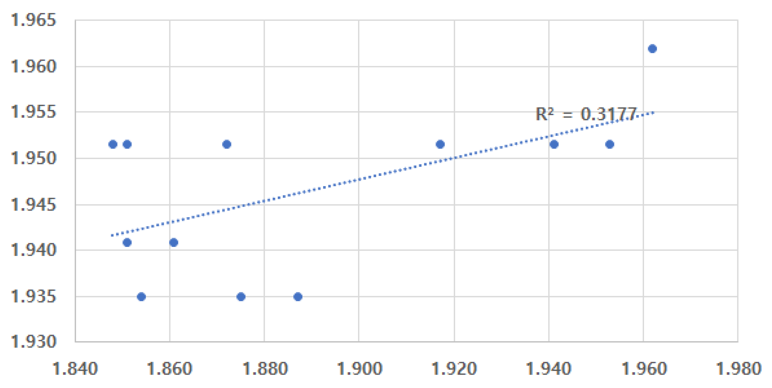
For further evaluation, we prepared the actual production time of product-G, which had a similar production volume to product-A, …, F. As described in Section 4.5 on utilizing production time improvement rates, we applied the products A, B, C, D, E, and F production improvement rates to product-G’s production starting in month M+0 to produce a time series forecast1 for product-G’s production time. Similarly, we applied the products A and A1 production improvement rates to product-G to produce another time series forecast2 for product-G’s production time. The correlation coefficients and R-squared values were calculated for the actual production time of product-G from M+0 to M+11 and the results of predictions 1 and 2, respectively. Table 11 shows the correlation coefficients between the actual production time of product-G and predictions 1 and 2. From the correlation coefficients, we can see that the production improvement rate resulting from prediction 1 is more similar to the actual rate. Figure 14 plots the R-squared values of the product-G actual and prediction 1 rates, and Figure 15 plots the R-squared values of the product-G actual and prediction 2 rates. From the R-squared values, it can be seen that the results of prediction 1, which is based on the production improvement rate of products with similar production volumes, are more similar to the actual results.
5. Conclusions
This study aimed to calculate the impact of productivity improvement in terms of production time based on historical data and apply it to future production planning. To account for the unique circumstances of each manufacturing plant and the possibility of redefined production volumes, we categorized production volumes into specific intervals and computed future predictions based on these volumes. This approach allows us to use baseline information generated by an APS for future production volume forecasts, aligning with projected demand. By incorporating improvements in production time into these productivity predictions, we can simulate future production capacity forecasts. While these forecasts may not be entirely accurate for future mass-produced products, they offer valuable insights for preparing for future factory operations and setting productivity improvement targets based on past performance. This methodology is particularly beneficial for manufacturing companies in equipment-based industries or those involving equipment-intensive processes when making decisions about expensive equipment purchases or factory expansions.
In this study, we calculated the production improvement rate for products with similar production volumes and analyzed the production improvement rate for products with the same base product. Productivity improvement activities are centered on products with high production volumes, and in order to measure the production improvement rate and use the current production improvement rate for future products to predict possible production volumes and capacity shortages, the production improvement rate of products with similar production volumes should be calculated and used.
In order to predict the future based on historical data, the goal is to identify models where the past and present situations are very similar, such as the similarity of process diagrams or production plans. Utilizing AI-based analytics in conjunction with big data can increase the similarity between reality and future predictions.
Author Contributions
Conceptualization, I.K. and J.J.; methodology, I.K.; software, I.K. and H.S.; validation, I.K., H.S. and J.R; formal analysis, I.K.; investigation, I.K., H.S. and J.R.; resources, I.K.; data curation, H.S. and J.R.; writing—original draft preparation, I.K.; writing—review and editing, J.J.; visualization, I.K.; supervision, I.K.; project administration, J.J.; funding acquisition, J.J. All authors have read and agreed to the published version of the manuscript.
Funding
This research was supported by the SungKyunKwan University and the BK21 FOUR (Graduate School Innovation) funded by the Ministry of Education (MOE, Republic of Korea) and the National Research Foundation of Korea (NRF).
Institutional Review Board Statement
Not applicable.
Informed Consent Statement
Not applicable.
Data Availability Statement
Not applicable.
Acknowledgments
This research was supported by the SungKyunKwan University and the BK21 FOUR (Graduate School Innovation) funded by the Ministry of Education (MOE, Korea) and the National Research Foundation of Korea (NRF). Moreover, this work was supported by the MSIT (Ministry of Science and ICT), Korea, under the ICT Creative Consilience Program (IITP-2023-2020-0-01821) supervised by the IITP (Institute for Information and Communications Technology Planning and Evaluation).
Conflicts of Interest
The authors declare no conflict of interest.
References
- Bellgran, M.; Säfsten, K. Production Development-Design and Operation of Production Systems; Springer: Berlin/Heidelberg, Germany, 2010. [Google Scholar]
- Palange, A.; Dhatrak, P. Lean manufacturing a vital tool to enhance productivity in manufacturing. Mater. Today Proc. 2021, 46, 729–736. [Google Scholar] [CrossRef]
- Andersson, C.; Bellgran, M. On the complexity of using performance measures: Enhancing sustained production improvement capability by combining OEE and productivity. J. Manuf. Syst. 2015, 35, 144–154. [Google Scholar] [CrossRef]
- Rohani, J.M.; Zahraee, S.M. Production line analysis via value stream mapping: A lean manufacturing process of color industry. Procedia Manuf. 2015, 2, 6–10. [Google Scholar] [CrossRef]
- Sharma, K.M.; Lata, S. Effectuation of lean tool “5s” on materials and work space efficiency in a copper wire drawing micro-scale industry in India. Mater. Today Proc. 2018, 5, 4678–4683. [Google Scholar] [CrossRef]
- Veres, C.; Marian, L.; Moica, S.; Al-Akel, K. Case study concerning 5S method impact in an automotive company. Procedia Manuf. 2018, 22, 900–905. [Google Scholar] [CrossRef]
- Nallusamy, S. Execution of lean and industrial techniques for productivity enhancement in a manufacturing industry. Mater. Today Proc. 2021, 37, 568–575. [Google Scholar] [CrossRef]
- Arunagiri, P.; Suresh, P.; Jayakumar, V. Assessment of hypothetical correlation between the various critical factors for lean systems in automobile industries. Mater. Today Proc. 2020, 33, 35–38. [Google Scholar] [CrossRef]
- Bueno, A.; Godinho Filho, M.; Frank, A.G. Smart production planning and control in the Industry 4.0 context: A systematic literature review. Comput. Ind. Eng. 2020, 149, 106774. [Google Scholar] [CrossRef]
- Bonney, M. Reflections on production planning and control (PPC). Gest. Prod. 2000, 7, 181–207. [Google Scholar] [CrossRef]
- Wiendahl, H.H.; Von Cieminski, G.; Wiendahl, H.P. Stumbling blocks of PPC: Towards the holistic configuration of PPC systems. Prod. Plan. Control 2005, 16, 634–651. [Google Scholar] [CrossRef]
- Yin, Y.; Stecke, K.E.; Li, D. The evolution of production systems from Industry 2.0 through Industry 4.0. Int. J. Prod. Res. 2018, 56, 848–861. [Google Scholar] [CrossRef]
- Olhager, J.; Rudberg, M. Linking manufacturing strategy decisions on process choice with manufacturing planning and control systems. Int. J. Prod. Res. 2002, 40, 2335–2351. [Google Scholar] [CrossRef]
- Olhager, J. Evolution of operations planning and control: From production to supply chains. Int. J. Prod. Res. 2013, 51, 6836–6843. [Google Scholar] [CrossRef]
- Jacobs, R.F.; Berry, W.L.; Whybark, D.C.; Vollmann, T.E. Manufacturing planning and control for supply chain management: The CPIM Reference; McGraw-Hill Education: New York, NY, USA, 2018. [Google Scholar]
- Rondeau, P.; Litteral, L.A. The evolution of manufacturing planning and control systems: From reorder point to enterprise resource planning. Prod. Inventory Manag. J. 2001, 42. Available online: https://digitalcommons.butler.edu/cob_papers/41 (accessed on 27 September 2023).
- Nahmias, S.; Olsen, T.L. Production and Operations Analysis; Waveland Press: Long Grove, IL, USA, 2015. [Google Scholar]
- Lee, H.Y. Development of a Simulation-Based Smart-FAB Production Operating System Framework for the FAB Industries; Korea Advanced Institute of Science & Technology (KAIST): Daejeon, Republic of Korea, 2011. [Google Scholar]
- Ivert, L.K.; Jonsson, P. The potential benefits of advanced planning and scheduling systems in sales and operations planning. Ind. Manag. Data Syst. 2010, 110, 659–681. [Google Scholar] [CrossRef]
- Hvolby, H.H.; Steger-Jensen, K. Technical and industrial issues of Advanced Planning and Scheduling (APS) systems. Comput. Ind. 2010, 61, 845–851. [Google Scholar] [CrossRef]
- Venkatesh, J. An Introduction to Total Productive Maintenance (TPM); The Plant Maintenance Resource Center: Como, Italy, 2007; pp. 3–20. [Google Scholar]
- Chan, F.; Lau, H.; Ip, R.; Chan, H.; Kong, S. Implementation of total productive maintenance: A case study. Int. J. Prod. Econ. 2005, 95, 71–94. [Google Scholar] [CrossRef]
- Swanson, L. Linking maintenance strategies to performance. Int. J. Prod. Econ. 2001, 70, 237–244. [Google Scholar] [CrossRef]
- Agustiady, T.K.; Cudney, E.A. Total productive maintenance. In Total Quality Management & Business Excellence; Routledge: London, UK, 2018; pp. 1–8. [Google Scholar]
- Adesta, E.Y.; Prabowo, H.A.; Agusman, D. Evaluating 8 pillars of Total Productive Maintenance (TPM) implementation and their contribution to manufacturing performance. IOP Conf. Ser. Mater. Sci. Eng. 2018, 290, 012024. [Google Scholar] [CrossRef]
- Attri, R.; Grover, S.; Dev, N.; Kumar, D. Analysis of barriers of total productive maintenance (TPM). Int. J. Syst. Assur. Eng. Manag. 2013, 4, 365–377. [Google Scholar] [CrossRef]
- Banga, H.K.; Kumar, R.; Kumar, P.; Purohit, A.; Kumar, H.; Singh, K. Productivity improvement in manufacturing industry by lean tool. Mater. Today Proc. 2020, 28, 1788–1794. [Google Scholar] [CrossRef]
- Pagliosa, M.; Tortorella, G.; Ferreira, J.C.E. Industry 4.0 and Lean Manufacturing: A systematic literature review and future research directions. J. Manuf. Technol. Manag. 2021, 32, 543–569. [Google Scholar] [CrossRef]
- Dillon, A.P. A Study of the Toyota Production System: From an Industrial Engineering Viewpoint; Routledge: Oxfordshire, UK, 2019. [Google Scholar]
- Anoop, G.; Muhammed, V.S. A Brief Overview on Toyota Production System (TPS). Int. J. Res. Appl. Sci. Eng. Technol. 2020, 8, 2505–2509. [Google Scholar]
- Mabkhot, M.M.; Al-Ahmari, A.M.; Salah, B.; Alkhalefah, H. Requirements of the smart factory system: A survey and perspective. Machines 2018, 6, 23. [Google Scholar] [CrossRef]
- Meerkov, S.M.; Yan, C.B. Production lead time in serial lines: Evaluation, analysis, and control. IEEE Trans. Autom. Sci. Eng. 2014, 13, 663–675. [Google Scholar] [CrossRef]
- Rahman, S.u. Theory of constraints: A review of the philosophy and its applications. Int. J. Oper. Prod. Manag. 1998, 18, 336–355. [Google Scholar] [CrossRef]
- Scholl, A.; Voß, S. Simple assembly line balancing—Heuristic approaches. J. Heuristics 1997, 2, 217–244. [Google Scholar] [CrossRef]
- Prasad, S.; Khanduja, D.; Sharma, S.K. A study on implementation of lean manufacturing in Indian foundry industry by analysing lean waste issues. Proc. Inst. Mech. Eng. Part B J. Eng. Manuf. 2018, 232, 371–378. [Google Scholar] [CrossRef]
- Tersine, R.J.; Hummingbird, E.A. Lead-time reduction: The search for competitive advantage. Int. J. Oper. Prod. Manag. 1995, 15, 8–18. [Google Scholar] [CrossRef]
- Ghazavi, M.; Eghbali, A.H. New geometric average method for calculation of ultimate bearing capacity of shallow foundations on stratified sands. Int. J. Geomech. 2013, 13, 101–108. [Google Scholar] [CrossRef]
Figure 1.
APS system organization and production operations area.
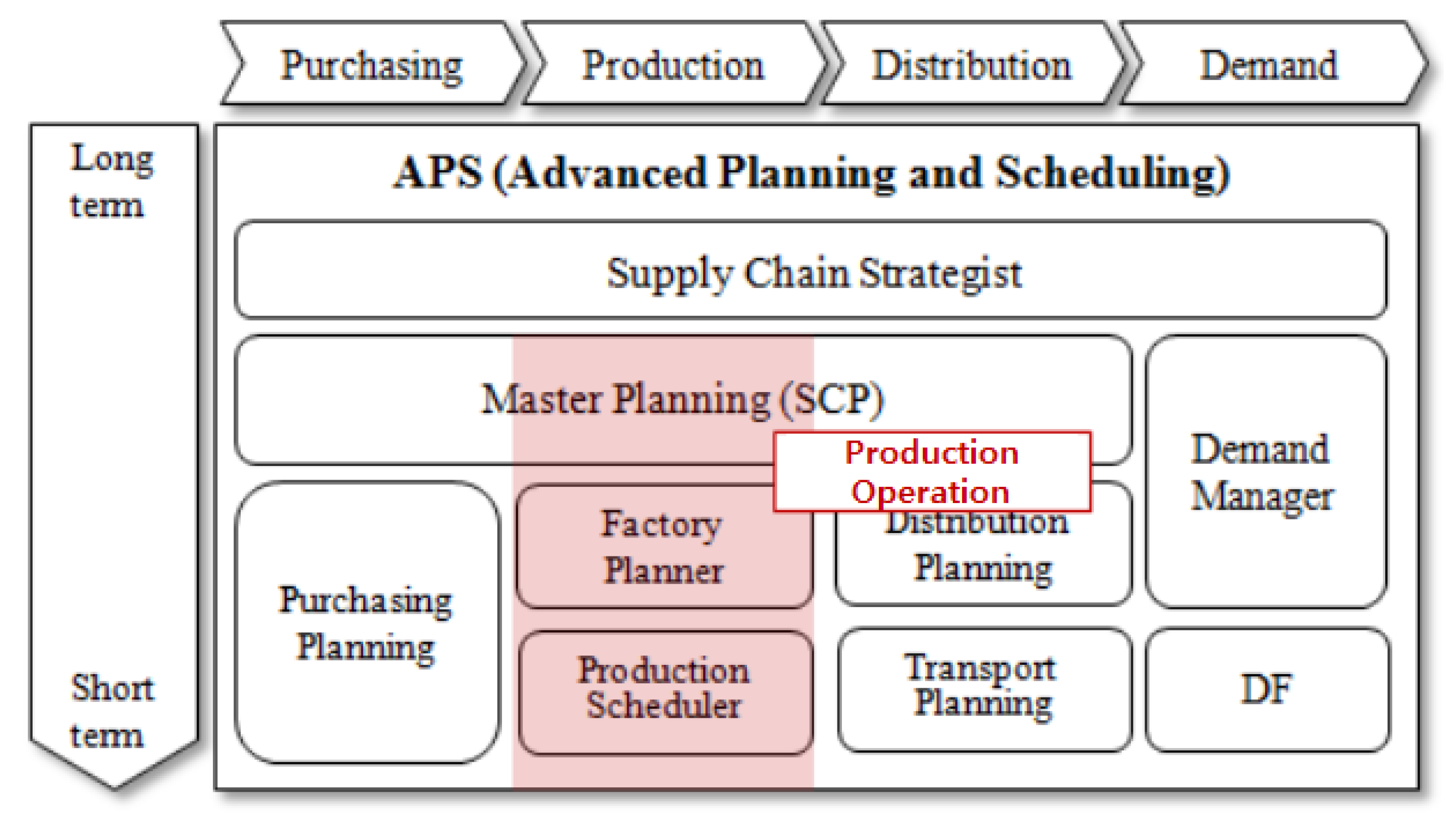
Figure 2.
Overall equipment effectiveness and the six main losses.
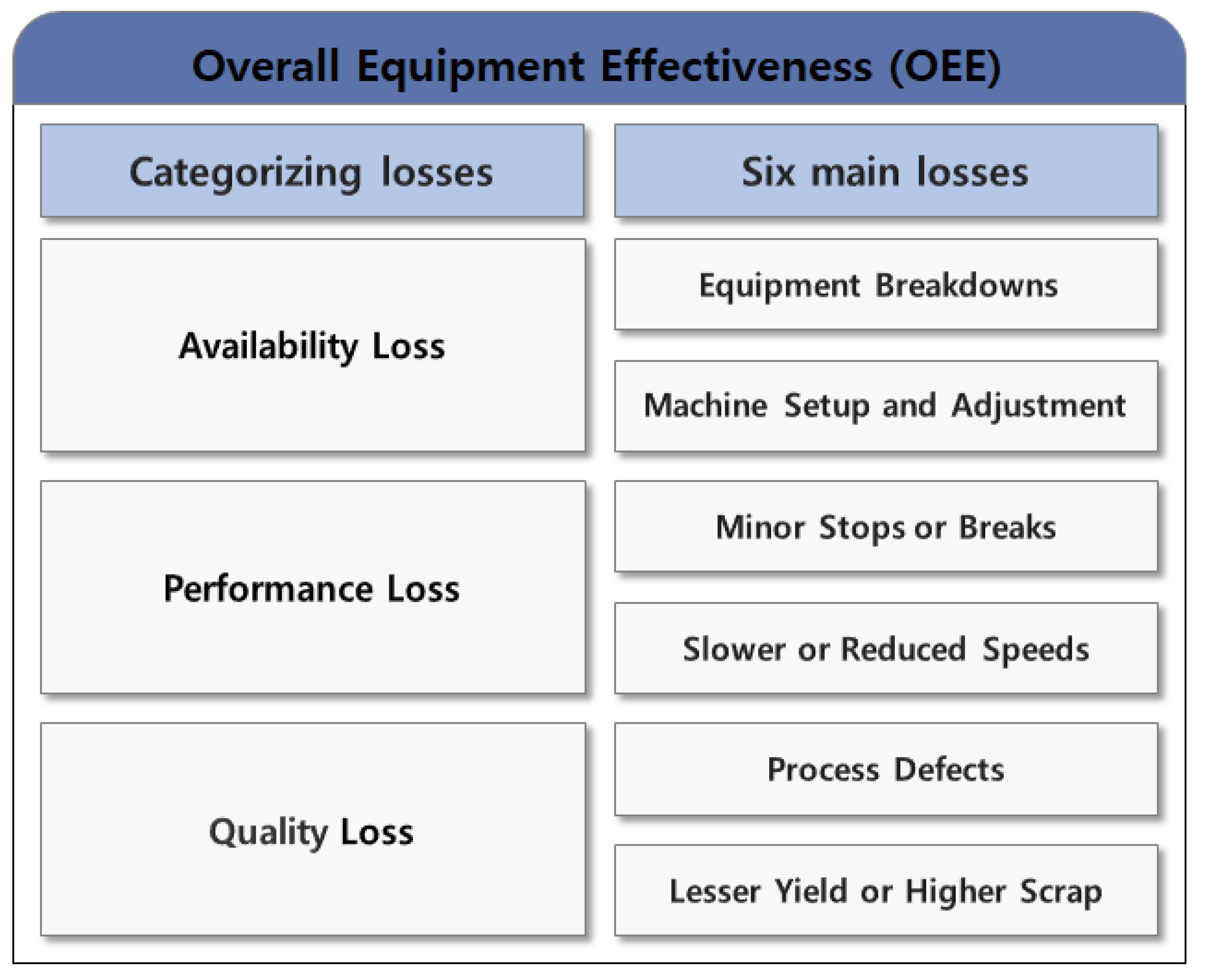
Figure 3.
The sum of the L/T for each process.

Figure 4.
Procedure for calculating production lead time improvement rate.
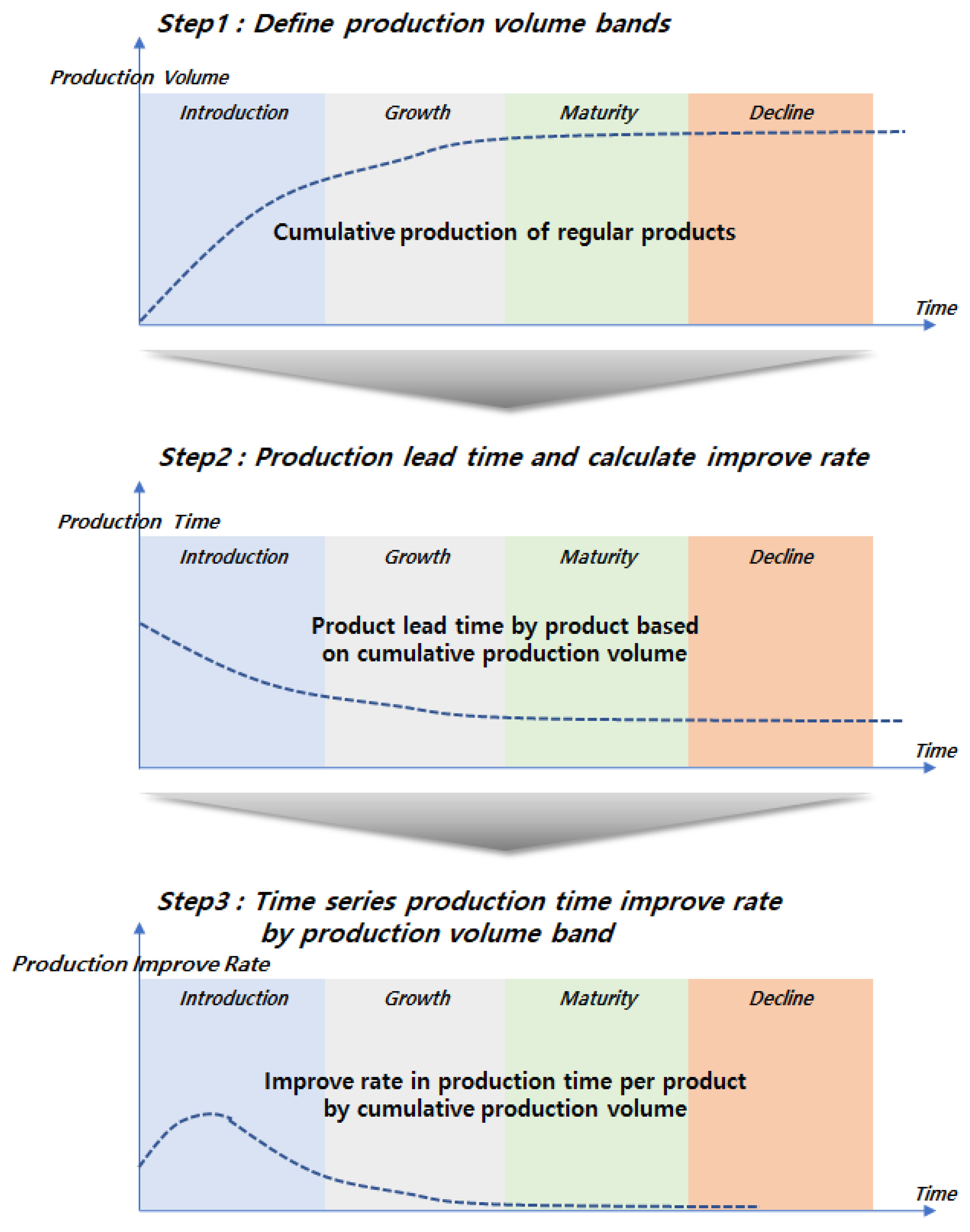
Figure 5.
L/T improvement rate and utilization based on production volume.
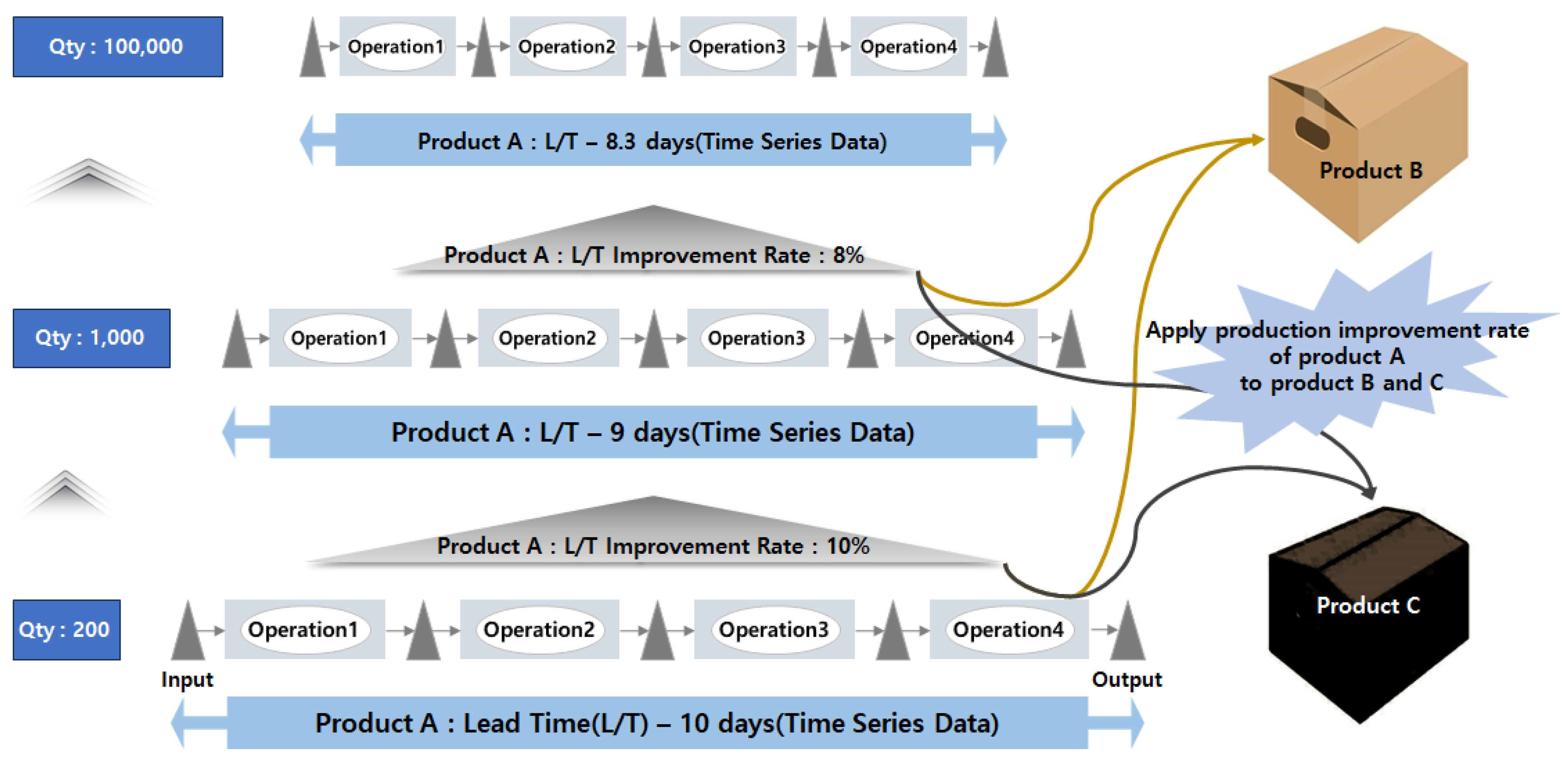
Figure 6.
Defining bins for production planning patterns. (Example of monthly production variation
for low volume products in green, Medium volume products in red, and high volume products in
blue).
Figure 6.
Defining bins for production planning patterns. (Example of monthly production variation
for low volume products in green, Medium volume products in red, and high volume products in
blue).
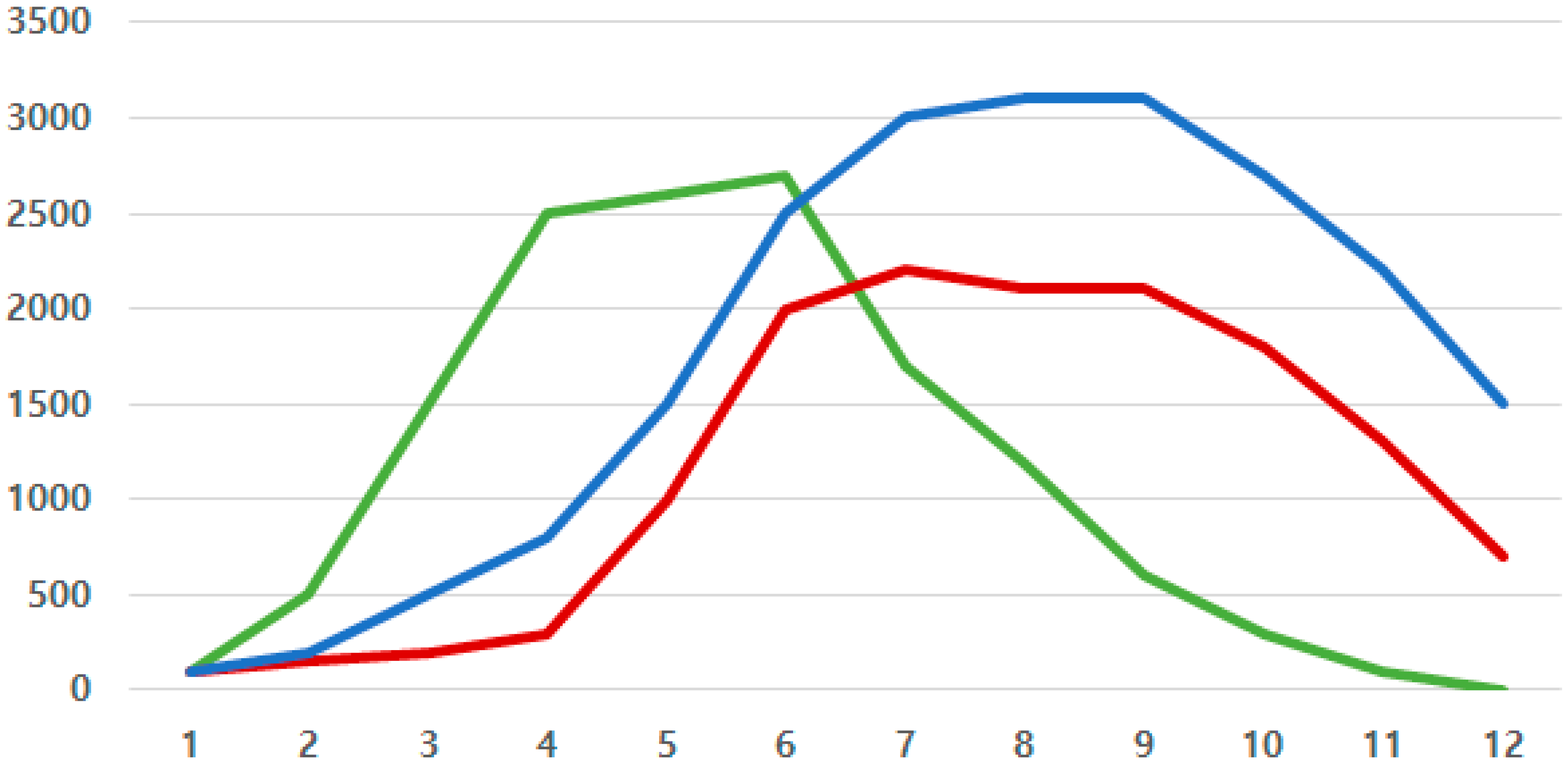
Figure 7.
Lead time improvement rate calculation data processing.
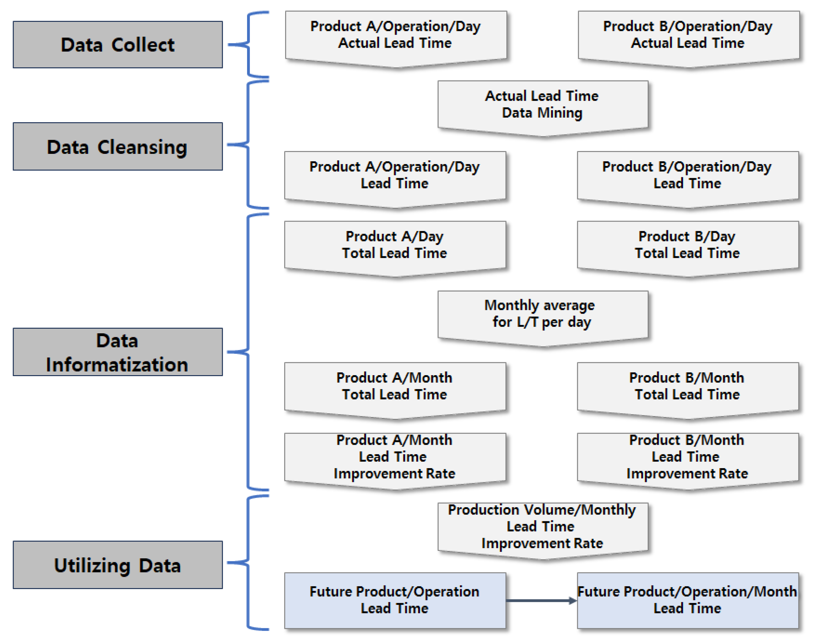
Figure 8.
Production time by product.

Figure 9.
Production time improvement rate by product.
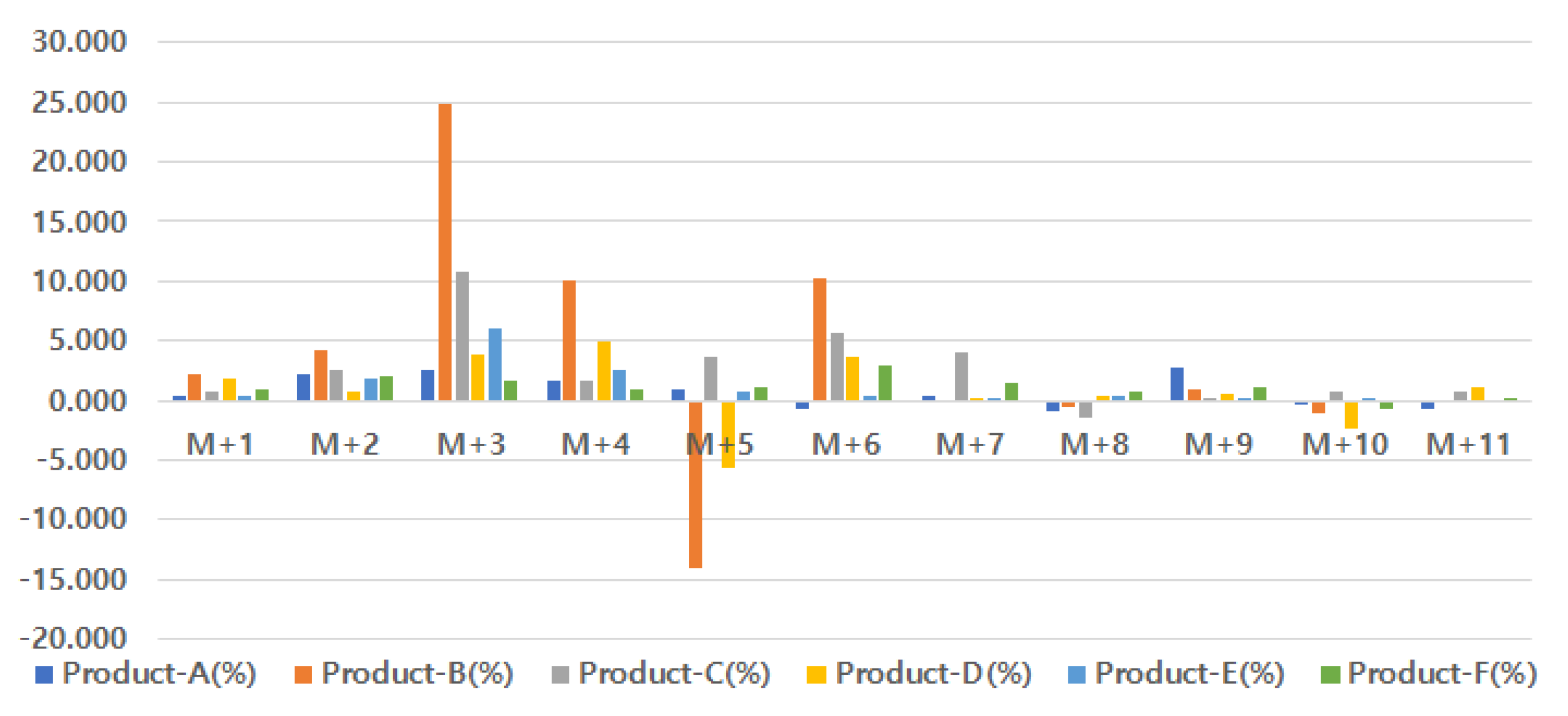
Figure 10.
Production time improvement rate for products with similar production volumes (high volume).
Figure 10.
Production time improvement rate for products with similar production volumes (high volume).

Figure 11.
Improvement rate (harmonic mean).
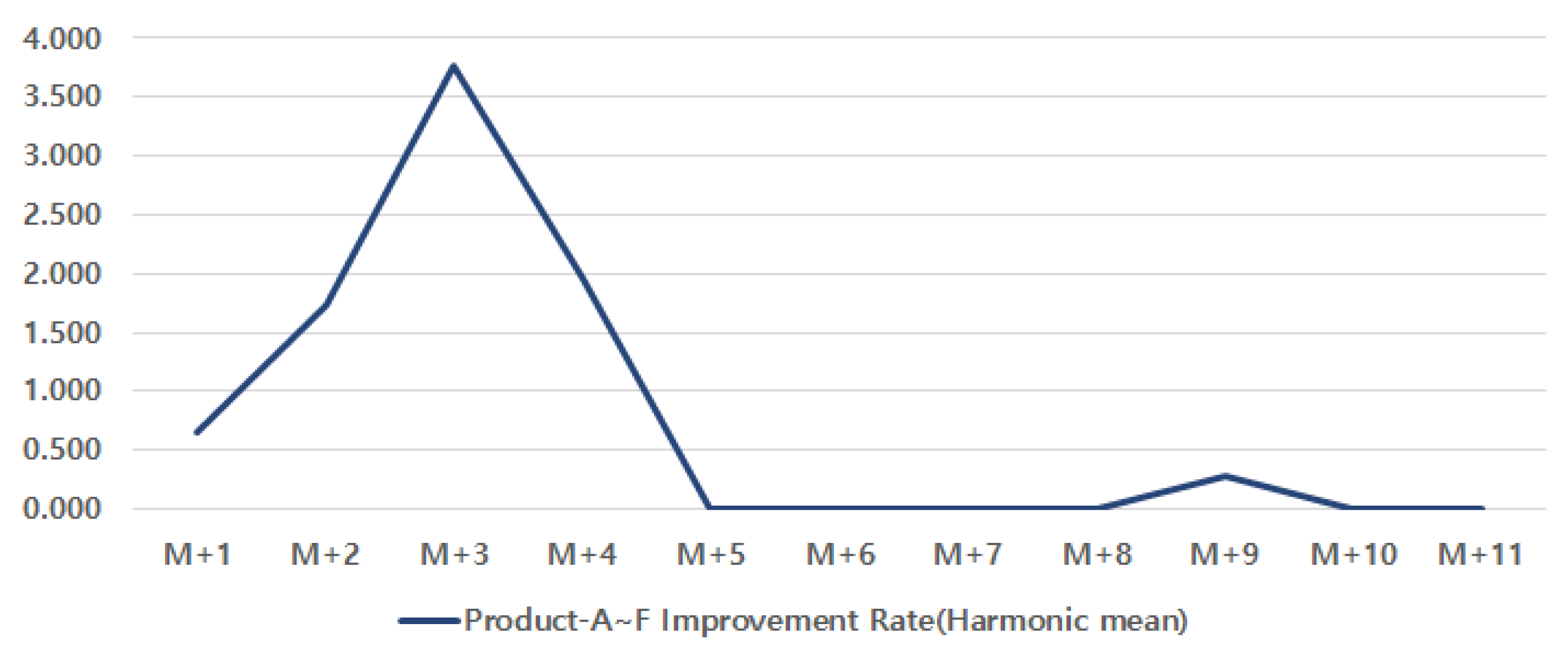
Figure 12.
Production time improvement rate for the same base product.
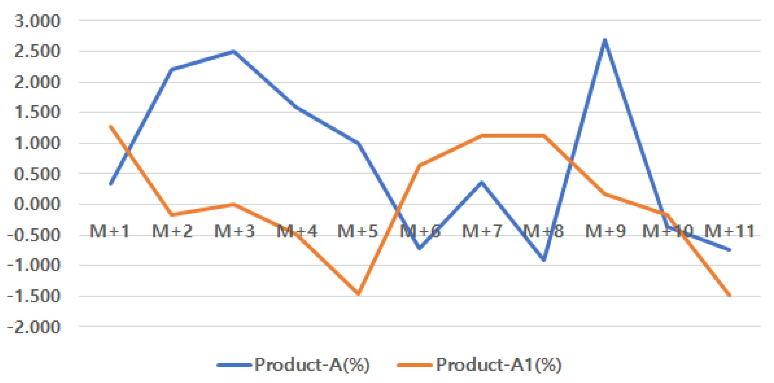
Figure 13.
Product-A, A1 improvement rate (harmonic mean).

Figure 14.
R-squared values for product-G and prediction 1.
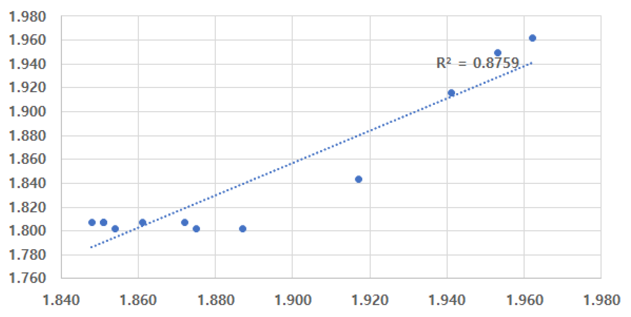
Figure 15.
R-squared values for product-G and prediction 2.

Table 1.
Total productive maintenance (TPM).
| TPM | |
|---|---|
| Object | Equipment (input and cause) |
| Means of attaining goal | Employee participation and equipment oriented |
| Target | Elimination of losses and waste |
Table 2.
Defining bins for production planning patterns.
| Distinguish | Monthly Production (Units) | Yearly Production (Units) | Note |
|---|---|---|---|
| Low | 0 to 500 | Under 5000 | Of the two divisions of production, yearly production is preferred |
| Medium | Over 500 to Under 10,000 | Over 5000 to Under 100,000 | |
| High | Over 10,000 | Over 100,000 |
Table 3.
DB server hardware environment.
| Hardware | Performance |
|---|---|
| CPU | Intel Xeon Gold 5220 @ 2.20 GHz |
| RAM | 512 GB |
| STORAGE | 50 TB (SSD) |
Table 4.
Notebook hardware environment.
| Hardware | Performance |
|---|---|
| CPU | Intel i7-6700 @ 3.40 GHz |
| RAM | 32 GB |
| STORAGE | 256 GB (SSD) |
Table 5.
Notebook development environment.
| Type | |
|---|---|
| OS | Windows 11 Home 22H2 |
| DBMS | Oracle 19 Client |
| Development Languages | Oracle PL/SQL |
| Development Tools | SQL Developer |
Table 6.
Products A, B, C, D, E, F production time.
| Production Time | ||||||
|---|---|---|---|---|---|---|
| Month | Product-A | Product-B | Product-C | Product-D | Product-E | Product-F |
| M+0 | 2.970 | 2.359 | 3.045 | 3.321 | 2.024 | 2.064 |
| M+1 | 2.960 | 2.309 | 3.023 | 3.259 | 2.016 | 2.046 |
| M+2 | 2.895 | 2.211 | 2.945 | 3.236 | 1.978 | 2.004 |
| M+3 | 2.823 | 1.663 | 2.624 | 3.114 | 1.858 | 1.972 |
| M+4 | 2.777 | 1.497 | 2.581 | 2.962 | 1.812 | 1.954 |
| M+5 | 2.750 | 1.708 | 2.486 | 3.130 | 1.799 | 1.933 |
| M+6 | 2.770 | 1.532 | 2.344 | 3.013 | 1.793 | 1.876 |
| M+7 | 2.760 | 1.532 | 2.250 | 3.004 | 1.791 | 1.848 |
| M+8 | 2.785 | 1.541 | 2.285 | 2.994 | 1.785 | 1.834 |
| M+9 | 2.710 | 1.526 | 2.279 | 2.976 | 1.7838 | 1.813 |
| M+10 | 2.720 | 1.542 | 2.261 | 3.049 | 1.782 | 1.827 |
| M+11 | 2.740 | 1.543 | 2.246 | 3.0152 | 1.782 | 1.823 |
Table 7.
Products A, B, C, D, E, F production time improvement rate.
| Improvement Rate (%) for Products with Similar Production Volumes (High Volume) | |||||||
|---|---|---|---|---|---|---|---|
| Month | Product-A | Product-B | Product-C | Product-D | Product-E | Product-F | Products A∼F (Harmonic Mean) |
| M+1 | 0.337 | 2.120 | 0.732 | 1.855 | 0.366 | 0.858 | 0.648 |
| M+2 | 2.196 | 4.224 | 2.581 | 0.724 | 1.880 | 2.076 | 1.727 |
| M+3 | 2.504 | 24.785 | 10.884 | 3.764 | 6.061 | 1.590 | 3.771 |
| M+4 | 1.594 | 9.982 | 1.631 | 4.862 | 2.518 | 0.898 | 1.963 |
| M+5 | 0.990 | −14.061 | 3.692 | −5.671 | 0.718 | 1.087 | 0.000 |
| M+6 | −0.727 | 10.307 | 5.708 | 3.757 | 0.339 | 2.930 | 0.000 |
| M+7 | 0.361 | 0.000 | 4.010 | 0.289 | 0.100 | 1.509 | 0.000 |
| M+8 | −0.906 | −0.588 | −1.533 | 0.350 | 0.307 | 0.766 | 0.000 |
| M+9 | 2.693 | 0.935 | 0.228 | 0.575 | 0.080 | 1.158 | 0.287 |
| M+10 | −0.369 | −1.042 | 0.798 | −2.432 | 0.122 | −0.781 | 0.000 |
| M+11 | −0.735 | −0.032 | 0.681 | 1.102 | 0.000 | 0.194 | 0.000 |
Table 8.
Utilizing improvement rate results.
| Time Series Production Time Information | ||
|---|---|---|
| Month | Improvement Rate | Production Time |
| M+0 | 0.000% | 4.000 |
| M+1 | 0.648% | 3.974 |
| M+2 | 1.727% | 3.905 |
| M+3 | 3.771% | 3.758 |
| M+4 | 1.963% | 3.684 |
| M+5 | 0.000% | 3.684 |
| M+6 | 0.000% | 3.684 |
| M+7 | 0.000% | 3.684 |
| M+8 | 0.000% | 3.684 |
| M+9 | 0.287% | 3.674 |
| M+10 | 0.000% | 3.674 |
| M+11 | 0.000% | 3.674 |
Table 9.
Previous experiment products A, A1 production time improvement rate.
| Product-A | Product-A1 | |||
|---|---|---|---|---|
| Month | Production Time | Improvement Rate | Production Time | Improvement Rate |
| M+0 | 2.97 | 0.624 | ||
| M+1 | 2.96 | 0.377% | 0.616 | 1.282% |
| M+2 | 2.895 | 2.196% | 0.617 | −0.162% |
| M+3 | 2.8225 | 2.504% | 0.617 | 0.000% |
| M+4 | 2.7775 | 1.594% | 0.620 | −0.486% |
| M+5 | 2.75 | 0.990% | 0.629 | −1.452% |
| M+6 | 2.77 | −0.727% | 0.625 | 0.636% |
| M+7 | 2.76 | 0.361% | 0.618 | 1.120% |
| M+8 | 2.785 | −0.906% | 0.611 | 1.133% |
| M+9 | 2.71 | 2.693% | 0.610 | 0.164% |
| M+10 | 2.72 | −0.369% | 0.611 | −0.164% |
| M+11 | 2.74 | −0.735% | 0.620 | −1.473% |
Table 10.
Previous experiment production time harmonic mean improvement rate.
| Production Time Improvement Rate for Products with Different Production Volumes (Low and High Volume) | |||
|---|---|---|---|
| Month | Product-A Improvement Rate | Product-A1 Improvement Rate | Improvement Rate (Harmonic Mean) |
| M+1 | 0.377% | 1.282% | 0.533% |
| M+2 | 2.196% | −0.162% | 0.000% |
| M+3 | 2.504% | 0.000% | 0.000% |
| M+4 | 1.594% | −0.486% | 0.000% |
| M+5 | 0.990% | −1.452% | 0.000% |
| M+6 | −0.727% | 0.636% | 0.000% |
| M+7 | 0.361% | 1.120% | 0.546% |
| M+8 | −0.906% | 1.133% | 0.000% |
| M+9 | 2.693% | 0.164% | 0.309% |
| M+10 | −0.369% | −0.164% | 0.000% |
| M+11 | −0.735% | −1.473% | 0.000% |
Table 11.
Correlation coefficient between actual production time and predicted value.
| Month | Product-G Actual Production Time | Products A∼F Improvement Rate | Product-G Predictions 1 | Products A, A1 Improvement Rate | Product-G Predictions 2 |
|---|---|---|---|---|---|
| M+0 | 1.962 | 0.000% | 1.962 | 0.000% | 1.962 |
| M+1 | 1.953 | 0.648% | 1.949 | 0.533% | 1.952 |
| M+2 | 1.941 | 1.727% | 1.916 | 0.000% | 1.952 |
| M+3 | 1.917 | 3.771% | 1.843 | 0.000% | 1.952 |
| M+4 | 1.872 | 1.963% | 1.807 | 0.000% | 1.952 |
| M+5 | 1.848 | 0.000% | 1.807 | 0.000% | 1.952 |
| M+6 | 1.851 | 0.000% | 1.807 | 0.000% | 1.952 |
| M+7 | 1.851 | 0.000% | 1.807 | 0.546% | 1.941 |
| M+8 | 1.861 | 0.000% | 1.807 | 0.000% | 1.941 |
| M+9 | 1.887 | 0.287% | 1.802 | 0.309% | 1.935 |
| M+10 | 1.875 | 0.000% | 1.802 | 0.000% | 1.935 |
| M+11 | 1.854 | 0.000% | 1.802 | 0.000% | 1.935 |
| Prediction 1 correlation coefficient | 0.936 | Prediction 2 correlation coefficient | 0.564 |
Disclaimer/Publisher’s Note: The statements, opinions and data contained in all publications are solely those of the individual author(s) and contributor(s) and not of MDPI and/or the editor(s). MDPI and/or the editor(s) disclaim responsibility for any injury to people or property resulting from any ideas, methods, instructions or products referred to in the content. |
© 2023 by the authors. Licensee MDPI, Basel, Switzerland. This article is an open access article distributed under the terms and conditions of the Creative Commons Attribution (CC BY) license (https://creativecommons.org/licenses/by/4.0/).
Share and Cite
MDPI and ACS Style
Ki, I.; Song, H.; Ryu, J.; Jeong, J. Production Improvement Rate with Time Series Data on Standard Time at Manufacturing Sites. Appl. Sci. 2023, 13, 10937. https://doi.org/10.3390/app131910937
AMA Style
Ki I, Song H, Ryu J, Jeong J. Production Improvement Rate with Time Series Data on Standard Time at Manufacturing Sites. Applied Sciences. 2023; 13(19):10937. https://doi.org/10.3390/app131910937
Chicago/Turabian StyleKi, Injong, Hasup Song, Jihyeok Ryu, and Jongpil Jeong. 2023. "Production Improvement Rate with Time Series Data on Standard Time at Manufacturing Sites" Applied Sciences 13, no. 19: 10937. https://doi.org/10.3390/app131910937
Note that from the first issue of 2016, this journal uses article numbers instead of page numbers. See further details here.