Abstract
In this study, we identified the different causes of odor problems and their associated discomfort. We also recognized the significance of public health and environmental concerns. To address odor issues, it is vital to conduct precise analysis and comprehend the root causes. We suggested a hybrid model of a Convolutional Neural Network (CNN) and Transformer called the CNN–Transformer to tackle this challenge and assessed its effectiveness. We utilized a dataset containing 120,000 samples of odor to compare the performance of CNN+LSTM, CNN, LSTM, and ELM models. The experimental results show that the CNN+LSTM hybrid model has an accuracy of 89.00%, precision of 89.41%, recall of 91.04%, F1-score of 90.22%, and RMSE of 0.28, with a large prediction error. The CNN+Transformer hybrid model had an accuracy of 96.21%, precision and recall of 94.53% and 94.16%, F1-score of 94.35%, and RMSE of 0.27, showing a low prediction error. The CNN model had an accuracy of 87.19%, precision and recall of 89.41% and 91.04%, F1-score of 90.22%, and RMSE of 0.23, showing a low prediction error. The LSTM model had an accuracy of 95.00%, precision and recall of 92.55% and 94.17%, F1-score of 92.33%, and RMSE of 0.03, indicating a very low prediction error. The ELM model performed poorly with an accuracy of 85.50%, precision and recall of 85.26% and 85.19%, respectively, and F1-score and RMSE of 85.19% and 0.31, respectively. This study confirms the suitability of the CNN–Transformer hybrid model for odor analysis and highlights its excellent predictive performance. The employment of this model is expected to be advantageous in addressing odor problems and mitigating associated public health and environmental concerns.
1. Introduction
In modern society, various factors such as industrial processes, landfills, livestock production, agricultural activities, and automobile emissions contribute to the generation of unpleasant odors. These odors not only cause discomfort in daily life but also raise concerns about important issues in public health and the environment. To address odor-related problems, it is necessary to accurately analyze the causes of odor and the extent and nature of odor emissions.
Recent research has applied machine learning and deep learning techniques to odor analysis, enabling accurate and efficient odor detection and classification. Previous studies have mainly used machine learning algorithms such as Convolutional Neural Networks (CNNs) and Long Short-Term Memory (LSTM) to analyze odor data and evaluate their performances [1,2,3]. CNNs have been particularly effective in odor classification, as they extract data features and perform classification simultaneously, enabling rapid and accurate classification. Furthermore, CNNs can effectively process data by learning spatial relationships. However, CNNs require large amounts of data and high computational power, and they have low interpretability, making it difficult to understand the basis for classification [4]. Random Forest (RF) [5] evaluates the importance of various features and provides generalized results without overfitting the training data. RF demonstrates stable performance even with relatively small datasets. However, RF is relatively slow and memory intensive when dealing with large amounts of data, and its interpretability is limited. LSTM is specialized in handling time series data and is useful for predicting current odor patterns by remembering previous information [6]. LSTM performs well in modeling time series data and is suitable for handling odor data with temporal dependencies. However, LSTM requires high computational costs and is effective when trained on large-scale datasets. Additionally, interpreting the internal workings of LSTM is challenging [7]. Stacked Autoencoder (SAE) is an unsupervised learning technique that automatically learns features from input data and extracts latent patterns. SAE can remove noise and variability in data, enabling reliable odor classification [8]. However, SAE models perform effective learning on large-scale datasets but may show limited performance in the presence of data scarcity. Ensemble techniques combine multiple models to improve accuracy and generalization. CNN-based ensembles learn [9] various features and ensure model diversity, enhancing the accuracy of odor classification. However, ensemble models require more computational resources, and training and inference with multiple models may take more time [10].
Therefore, this study aims to propose a neural network architecture that combines CNN and Transformer, and evaluate its performance in odor analysis. Transformer provides efficient and parameter-effective modeling compared to traditional sequence modeling, and combining it with CNN is expected to build a more powerful odor analysis model. To assess the model’s performance, it will be compared and evaluated against CNN+LSTM hybrid models, CNN models, LSTM models, ELM models, and the proposed CNN–Transformer hybrid model. Additionally, performance metrics such as accuracy, precision, recall, F1 score, and the model’s predictive ability will be compared by measuring the RMSE value.
To achieve this, this study will construct a CNN–Transformer hybrid model using publicly available odor data consisting of 120,000 samples and evaluate the performance of the model.
The structure of this paper is as follows. Section 2 explains the basics of the CNN–Transformer hybrid model proposed in this study and the CNN+LSTM hybrid model, CNN model, LSTM model, ELM model, and the proposed CNN–Transformer for comparative analysis. In Section 3, this paper designs and applies the structures of the CNN+LSTM hybrid model, CNN model, LSTM model, ELM model, and the newly proposed CNN–Transformer hybrid model. Section 4 describes the experimental results. Finally, Section 5 discusses the conclusion of this paper.
2. Research Methodology
To compare and evaluate the performance of each model, we aim to design and apply the structures of the CNN+LSTM hybrid model, CNN model, LSTM model, ELM model, and the proposed CNN–Transformer hybrid model.
2.1. CNN Model
Convolutional Neural Networks (CNNs) are deep learning models that excel at image recognition and pattern recognition. Basically, it has the ability to detect and extract local patterns from grid-like data, such as images. It is used in various fields such as image processing, computer vision, and natural language processing. The basic structures of CNN models include convolutions, pooling, activation functions, and fully connected layers [11].
The role of convolution here is to extract local features by applying a filter (kernel) to the input data. Filters perform multiplication operations while sliding the input data through a small window. This allows for the recognition of regional features in the input data. Equation (1) represents the computation of one element of the output feature map.
here, F(i, j) denotes the value at position (i, j) of the output feature map. W is the weight matrix of the filter (kernel), X is the input data matrix, and k, l are the filter indices. The role of pooling is to reduce the size of the extracted feature maps and preserve important information. In general, max pooling is the most common, and the largest value in a given area is selected and used as a representative value. Pooling can reduce the size of the space and the amount of computation. Here, Equation (2) is used in max pooling.
in this context, Y(i, j) represents the pooling result at position (i, j), and X refers to the pixel at positions 2i, 2j in the input data matrix. An activation function is used after the convolution and pooling operations to introduce nonlinearity. Typically, the Rectified Linear Unit (ReLU) function is used, which converts negative values to 0 and leaves positive values unchanged. This allows the model to learn nonlinear patterns.
F(i, j) = (W · X)(i, j) = ∑∑(W(k, l) · X(i + k, j + l))
Y(i, j) = max(X(2i, 2j), X(2i, 2j + 1), X(2i + 1, 2j), X(2i + 1, 2j + 1))
Therefore, the activation function, usually ReLU, is used as shown in Equation (3).
ReLU(x) = max(0, x)
The fully connected layer (FCL)takes the feature maps that have undergone convolution and pooling and flattens them into a one-dimensional vector. This vector is then fed into the fully connected layer to perform the final prediction. The fully connected layer is a layer where all neurons between the input and output are connected, enabling predictions for various class labels. The following Equation (4) represents the formula for the FCL, which calculates the values of the output neurons.
here, Z represents the value of the output neuron, W denotes the weight matrix, X represents the input vector, and b is the bias vector. The structure of a CNN consists of alternating convolutional layers and pooling layers. This configuration allows the network to learn abstract features at different levels. Typically, a fully connected layer is added at the end to perform the final prediction. The CNN learns and optimizes the weights of the filters through training, using the backpropagation algorithm to propagate errors and update the weights.
Z = W · X + b
2.2. LSTM Model
The Long Short-Term Memory (LSTM) Model is a type of recurrent neural network designed to process sequential data such as time series or sentences [12]. It addresses the issues of vanishing and exploding gradients while effectively capturing long-term dependencies. The LSTM model consists of a cell, an input gate, a forget gate, and an output gate. Each gate produces values between 0 and 1 using the sigmoid function to determine which information to retain and which to discard. The input gate decides how much information to remember based on the current time step’s input and the previous time step’s hidden state. The activation calculation for the input gate, as shown in Equation (5), is as follows:
here, i(t) represents the activation value of the input gate, Wi denotes the weight matrix for the input, h(t−1) is the previous time step’s hidden state (output of the previous memory cell), x(t) is the input at the current time step, bi is the bias vector for the input gate, and σ represents the sigmoid activation function. The forget gate determines how much information to discard from the previous cell state, enabling the learning of long-term dependencies. The activation calculation formula for the forget gate, as shown in Equation (6), is as follows:
here, f(t) represents the activation value of the forget gate, Wf denotes the weight matrix for the inputs, and bf represents the bias vector of the forget gate. The cell state is updated by combining the preserved information from the previous time step’s cell state with the selected candidate values through the input gate. The cell state plays a crucial role in storing important information with long-term significance. Updating the cell state involves determining how much information to preserve from the previous cell state, as shown in Equation (7).
here, C(t) represents the cell state at the current time step, ⊙ denotes element-wise multiplication, and g(t) performs the calculation of the candidate value for the cell at the current time step as described in Equation (8).
i(t) = σ(Wi · [h(t − 1), x(t)] + bi)
f(t) = σ(Wf · [h(t − 1), x(t)] + bf)
C(t) = f(t) ⊙ C(t − 1) + i(t) ⊙ g(t)
g(t) = tanh(Wc · [h(t − 1), x(t)] + bc)
The output gate determines what information to output based on the current time step’s input and the previous time step’s hidden state. Equation (9) calculates the activation value of the output gate:
here, o(t) represents the activation value of the output gate. Wo represents the weight matrix for the input, and bo represents the bias vector for the output gate. By multiplying the activation value of the output gate with the cell state, we obtain the final hidden state, which is then passed through the hyperbolic tangent function. Equation (10) calculates the hidden state (output) at the current time step.
here, h(t) represents the current time step’s hidden state (output of the current memory cell), ⊙ denotes element-wise multiplication, and tanh refers to the hyperbolic tangent activation function. These equations constitute the fundamental formulas and equations used in LSTM models. LSTM overcomes the limitations of traditional RNNs, such as the vanishing and exploding gradient problems, allowing it to capture long-term dependencies in time series data. It updates the input, output, cell state, and hidden state while preserving information and selectively providing relevant information. LSTM models process input sequences one step at a time, updating the cell state and hidden state at each step. This enables the capture of long-term dependencies and the learning of sequential patterns in data. LSTM is widely used in tasks such as time series prediction, machine translation, and natural language processing, and it serves as a critical component in deep learning.
o(t) = σ(Wo · [h(t − 1), x(t)] + bo)
h(t) = o(t) ⊙ tanh(C(t))
2.3. ELM Model
The Extreme Learning Machine (ELM) Model is a type of machine learning algorithm based on neural networks. Unlike traditional neural network models, ELM initializes the weight of the hidden layer randomly and calculates the weight of the output layer with only one training iteration. This characteristic allows ELM to provide fast learning speeds and a good generalization performance [13]. The structure of an ELM model consists of an input layer, a hidden layer, and an output layer. The input layer receives the given data, and the hidden layer, located between the input and output layers, calculates the output values of hidden neurons. The neurons in the hidden layer perform a nonlinear transformation on the input data, and the output layer calculates the final output based on the output values of the hidden layer. The basic concept of an ELM model is as follows: There is a hidden layer between the input and output layers, that has randomly initialized weights. The input data is passed to the hidden layer, and the neurons in the hidden layer calculate the output values through an activation function.
The output value H of the hidden layer is calculated using the input data X, the weights W1, and the bias b1, as shown in Equation (11).
here, g represents the activation function of the hidden layer. After calculating the output of the hidden layer using the input data, an ELM model computes the weights of the output layer by solving a system of linear equations. The calculation of the output layer weights is given by Equation (12). The output layer weights, W2, are calculated using the output values H of the hidden layer and the actual output values Y.
here, HT represents the transposition of the hidden layer output values H, and C is a term for regularization. The weights can be obtained using methods such as Least Squares or Pseudo-inverse. With the computed weights of the output layer, predictions for new input data can be performed. The prediction for new input data is given by Equation (13), where the new input data, X_new, is used along with the weights, W1, and bias, b1, of the hidden layer to calculate the output values, H_new, of the hidden layer. The predicted value, Y_pred, is then calculated using the weights, W2, of the output layer.
H = g(X · W1 + b1)
W2 = (HT · H + C)−1 · HT · Y
H_new = g(X_new · W1 + b1) Y_pred = H_new · W2
ELM offers fast learning speeds and a good generalization ability compared to traditional neural network algorithms. Additionally, ELM initializes the weights of the hidden layer randomly, reducing sensitivity to initial weight settings and eliminating the need for manual weight adjustment by users. Due to these characteristics, ELM can be effectively used in various fields, particularly for handling large-scale data and real-time predictions.
2.4. Transformer Model
The Transformer model is primarily used in natural language processing and exhibits excellent performance in various tasks such as machine translation, sentence generation, and question-answering [14,15]. It is based on the attention mechanism and has a structure that can handle sequence data without relying on recurrent neural networks (RNNs). This feature resolves the issue of long-term dependencies while significantly improving computational speed. The Transformer model consists of two main components: an encoder and the decoder. The encoder embeds the input sequence into a multidimensional space and performs the role of encoding information. It is composed of multiple encoder layers, each having the same structure. The encoder layer consists of some key components: the self-attention mechanism and feed-forward neural network. The decoder, relying on the output of the encoder, generates the output sequence. Similarly to the encoder, it is composed of multiple decoder layers with the same structure. The decoder layer consists of the self-attention mechanism, encoder–decoder attention mechanism, and the feed-forward neural network. To preserve the relative positional information between the input and output sequences, the transformer model employs positional encoding. During model training, the cross-entropy loss function is primarily used, and a backpropagation algorithm and optimizer are utilized, with the Adam optimizer being the most common choice. The Transformer model demonstrates exceptional performance in natural language processing tasks, particularly translation tasks. It allows parallel processing, effectively addresses long-term dependency issues, and exhibits a flexible structure that can handle tasks with different input and output lengths.
3. Models Design
In this study, we propose a hybrid neural network architecture called CNN–Transformer, which combines the CNN and Transformer models. The goal is to evaluate the performance of the proposed CNN–Transformer model in the context of odor analysis. To assess the effectiveness of the CNN–Transformer model, we compare it with other models, including the CNN+LSTM hybrid [16], CNN, LSTM [17], and ELM models [18]. Furthermore, we measure various performance metrics, such as accuracy, precision, recall, F1 score, and RMSE, to evaluate [19] the predictive capabilities of each model and compare their performance across these metrics. The CNN–Transformer hybrid model offers the advantage of incorporating both the CNN’s convolutional operations and Transformer’s attention mechanism, potentially capturing both local and global patterns in the input data. This combination aims to enhance the model’s ability to extract relevant features and capture long-term dependencies, leading to improved performance in odor analysis tasks.
3.1. Design of CNN+Transformer Hybrid Model
In this study, we apply a hybrid concept called CNN–Transformer, which combines the CNN and Transformer models, to design the basic structure of the CNN+LSTM hybrid, CNN, LSTM, and ELM models. Furthermore, we measure various performance metrics, such as accuracy, precision, recall, F1 score, and RMSE, to evaluate the predictive capabilities of each model and compare their performance across these metrics. The CNN–Transformer hybrid model offers the advantage of incorporating both the CNN’s convolutional operations and Transformer’s attention mechanism, potentially capturing both local and global patterns in the input data. This combination aims to enhance the model’s ability to extract relevant features and capture long-term dependencies, leading to improved performance in odor analysis tasks.
The CNN–Transformer hybrid neural network architecture in Figure 1 defines the input data format through the Input layer. The CNN layer extracts features from the sequence data by performing convolutional and pooling operations, followed by applying layer normalization. The output of the CNN layer serves as an input to the Transformer layer, which consists of attention layers and feed-forward neural network layers, followed by global average pooling. In this architecture, the output layer is a dense layer with two nodes, utilizing the sigmoid activation function.
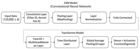
Figure 1.
CNN+Transformer hybrid neural network structure.
3.2. Design of CNN+LSTM Hybrid Model
The CNN+LSTM hybrid neural network structure in Figure 2 defines the shape of the input data through the Input layer; the Conv1D layer has 32 filters and a kernel size of five. The ReLU activation function is used to calculate the output. This is followed by down sampling using the MaxPooling1D layer and finally normalization via the Layer Normalization layer.
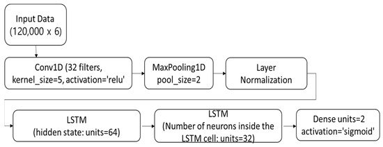
Figure 2.
CNN+LSTM hybrid neural network structure.
The LSTM layer consists of 64 and 32 units, respectively, and it is used to model the representation and internal state of the sequence data. Here, the units of 64 in the LSTM model represent the number of neurons within the LSTM cell. The LSTM cell controls the input, forget, and output gates, and updates the state of the memory cell. To accomplish this, multiple neurons are utilized.
The first units of 64 denotes the dimension of the hidden state, which is passed from the previous time step (t − 1) of the LSTM cell to the current time step (t) of the LSTM cell. The previous time step’s hidden state is fed as an input into the current time step’s LSTM cell and used in the current time step’s computations. The second unit of 64 represents the number of neurons within the current time step’s LSTM cell. These neurons are responsible for the calculations of the input, forget, and output gates, as well as the update of the memory cell, and units of 64 signifies that the LSTM cell contains 64 neurons internally.
This indicates that the LSTM cell has a certain level of model complexity that is suitable for a specific task or set of data. Therefore, the appearance of units of 64 twice serves to denote the dimension of the hidden state and the number of neurons within the LSTM cell, respectively.
Such configurations determine the model’s complexity and expressive power, and choosing an appropriate number of neurons can significantly impact the model’s performance and learning capabilities. Thus, in the given code, the CNN model and the LSTM model are used independently, where the output of the CNN model is passed as an input into the LSTM model for odor detection.
3.3. Design of CNN Model
The CNN model structure in Figure 3 is defined through the input layer, where the input data shape is specified. The Conv1D layer, Conv1D(32), is a one-dimensional convolutional layer that utilizes 32 filters. It has a kernel size of five and a stride of one. The ReLU activation function is used in this layer. The MaxPooling1D layer is a one-dimensional max-pooling layer with a pooling window size of two.
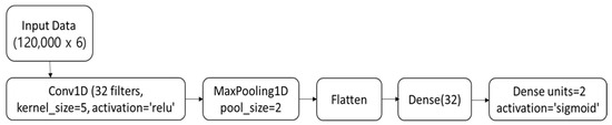
Figure 3.
CNN Model structure.
The flatten layer is responsible for transforming the multidimensional output, generated after passing it through the convolutional and max-pooling layers, into a one-dimensional shape. The Dense(32) layer is a fully connected layer with 32 units, and it employs the ReLU activation function. The Dense(2) layer is another fully connected layer with two units, and it utilizes the softmax activation function. This configuration is suitable for a classification problem with two classes, making it appropriate to be used as the output layer. The model’s output is a two-dimensional tensor representing a probability distribution, where each class is associated with a probability.
The neural network model structure in Figure 3 is created using the create_cnn_model() function in the given code. It is trained based on the provided dataset and compiled using the Adam optimizer and categorical cross-entropy loss function. After training, the model’s performance can be evaluated by assessing its accuracy and the loss function value.
3.4. Design of LSTM Model
The LSTM model structure in Figure 4 is defined through the input layer, where the input data shape is specified. The first LSTM layer has 32 units, and the return_sequences = True option is set to pass the output of the previous sequence to the next layer. The second layer also has 32 units, but return_sequences = False is configured to only return the output of the last sequence.
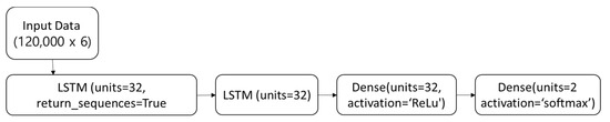
Figure 4.
LSTM Model structure.
The dense layer is a fully connected layer with 32 units and employs the ReLU activation function. The output layer is another fully connected layer with two units and uses the softmax activation function to output the classification results. This LSTM model, configured in this way, is trained and evaluated using the given dataset.
3.5. Design of ELM Model
The structure of the ELM (Extreme Learning Machine) model in Figure 5 is a simple neural network model composed of an input layer and a hidden layer. The model learns and predicts through the process of training. The input layer defines the shape of the input data. The size of the part that receives the input data is given by input_size, which corresponds to the number of features in the data. The hidden layer is the part that actually learns the weights and has a size given by hidden_size, representing the number of neurons in the hidden layer. The output of the hidden layer is obtained by performing weighted operations with the input layer and passing it through an activation function (tanh).
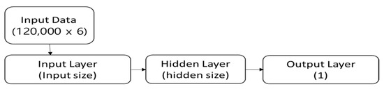
Figure 5.
ELM Model structure.
The output layer calculates the final output by performing weighted operations between the output of the hidden layer and the output weights. The size of the output layer is given as one, representing the predicted value in binary classification problems. Input weights refers to the weight matrix between the input layer and the hidden layer, with a size of (input_size, hidden_size). It represents the connection weights between the input layer and the hidden layer. Output weights refers to the weight matrix between the hidden layer and the output layer, with a size of (hidden_size, one). It represents the connection weights between the hidden layer and the output layer.
In the ELM model, the weights between the input layer and the hidden layer are randomly initialized. The hidden layer’s output and the output layer’s weights are then computed using the training data. After training, the model makes predictions using the test data.
4. Result of Implementation
The development environment for this study was constructed as shown in Table 1. In this study, the software environment for the experiment was developed using Python, 3.10 version, the artificial intelligence library used was the PyTorch-based MMDetection API, and the hardware environment was Windows 10 for OS, with an i9-9900 k for CPU, 128 GB of RAM, and 128 GB for the GPU. NVIDIA RTX 6000 was used, and a detailed environment is indicated in Table 1.

Table 1.
Configuration of Development Environment.
To evaluate the performance of odor analysis, we propose a hybrid neural network architecture called CNN–Transformer, which combines the CNN and Transformer models. The performance of the proposed CNN–Transformer hybrid model is compared and evaluated with other models, including the CNN+LSTM hybrid, CNN, LSTM, and ELM models, as shown in Figure 6.
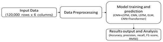
Figure 6.
Process of model training and performance evaluation.
Various performance metrics such as accuracy, precision, recall, F1 score, and RMSE are measured to assess the predictive capabilities of each model and compare their performance across these metrics. In this study, we utilize a publicly available dataset of 120,000 odor samples to construct the CNN–Transformer hybrid model and evaluate its performance. By comparing and evaluating the CNN–Transformer hybrid model against the other models, we aim to assess its effectiveness in odor analysis tasks and determine if it outperforms the existing models. The evaluation is based on performance metrics such as accuracy, precision, recall, F1 score, and RMSE, which provide insights into the model’s predictive capabilities and performance.
4.1. DataSet
In this study, a dataset was constructed using data collected from 1 January 2019 to 30 September 2019 from the Fine Dust and Odor Integrated Unmanned System (FDIUYS) installed in 15 locations in Cheongju-si, Chungcheongbuk-do. The details of the constructed dataset are shown in Table 2. Table 2 summarizes the types and quantities of data according to the given information. The total number of data samples is 120,000, which consists of 120 sets of time series data. Each time series of data is measured for 5 s and includes measurements for hydrogen sulfide, ammonia, benzene, toluene, and other substances. The total measurement duration is 600 s (10 min), and there is a total of 1000 data sets. Among these, 600 data sets are labeled as normal, while 400 data sets are labeled as abnormal. The data partitioning method in this paper used 80% of the total data for training, 10% for verification, and 10% for testing. In addition, training was conducted from the 1st to the 20th of every month, and the remaining 10 days were used for verification.
Table 2.
Construction of training data set.
Table 3 represents the normal and abnormal ranges for the given substances. Each substance has an average and standard deviation for both the normal and abnormal ranges. For example, the normal range for hydrogen sulfide is 0.4 ppm with an average of 0.3 ppm and a standard deviation of 0.1 ppm, while the abnormal range is 40 ppm with an average of 20 ppm and a standard deviation of 10 ppm. The same applies to Ammonia, Benzene, and Toluene, where the values and deviations for both normal and abnormal ranges are provided in the table.
Table 3.
Construction of training data set.
4.2. Results of Model Performance Evaluation
In Figure 7, we ran all epochs 50 times to find the one with the lowest data loss rate.
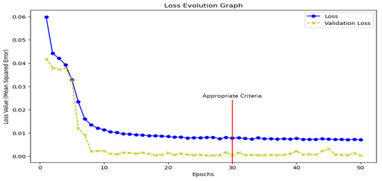
Figure 7.
Find the optimal high-parameter value for the AI model.
As you can see in the graph, we have the smallest loss rate at epoch 30. Therefore, we tested each AI model by using epoch 30 as the data training section.
As a performance test method for the AI models in this study, the structure of each model was applied to the format designed in Section 3.
In Table 4, we analyze the test results for CNN+LSTM, CNN+Transformer, CNN, LSTM, and Extreme Learning Machine (ELM). The CNN+LSTM hybrid model has an accuracy of 89.00%, indicating that it is predicting the data fairly accurately. The model appears to predict the benign class relatively accurately, with a precision of 89.41% and a recall of 91.04%. The F1-score is 90.22%, indicating a balanced performance of the model. However, it is important to consider that the prediction error is quite large with an RMSE of 0.28. The CNN+Transformer hybrid model has an accuracy of 96.21%, indicating that it is predicting the data very accurately, with precision and recall of 94.53% and 94.16%, respectively, showing high accuracy and balanced prediction. The F1-score is very high at 94.35%. It also has a low prediction error with an RMSE of 0.27. The accuracy of the CNN model is 87.19%, indicating that it is predicting the data somewhat accurately, and it tends to correctly predict the positive class, with precision and recall of 89.41% and 91.04%, respectively. The F1-score is 90.22%, indicating a balanced performance. It also has a low prediction error with an RMSE of 0.23. The accuracy of the LSTM model is quite high at 95.00%, with precision and recall of 92.55% and 94.17%, respectively, showing high accuracy and balanced prediction. The F1-score is high at 92.33%. It has a very low prediction error with an RMSE of 0.03. The ELM model performs poorly compared to the other models, with a moderate accuracy of 85.50%, and a moderate precision and recall of 85.26% and 85.19%, respectively. However, it has a low F1-score and RMSE of 85.19% and 0.31, respectively. Compared to other models, this model is relatively lacking in predictive results.
Table 4.
Results of evaluating the performance of artificial intelligence models.
As a result, the CNN+Transformer hybrid model performs the best, predicting the data very accurately. The LSTM model also performs well, and the CNN model performs moderately well. However, the CNN+LSTM and ELM models perform relatively poorly compared to the other models.
5. Conclusions
Currently, foul odor problems in modern society are caused by various causes, which can lead to people’s discomfort and public health and environmental problems. Therefore, to solve odor-related problems, various model experiments are needed to apply artificial intelligence models to identify the causes of odors.
In this study, we evaluated the analysis and prediction performance of various AI models by applying them to odor data collected from actual sites using various models. As a result of the experiments, the CNN+Transformer hybrid model showed the best performance and predicted the data very accurately. The LSTM model also performed well, and the CNN model performed moderately. However, the CNN+LSTM and ELM models showed relatively poor prediction results compared to other models.
Therefore, to cope with odor-related problems, it can be useful to consider the CNN+Transformer hybrid model when selecting a data prediction model. This model shows better prediction performance with a smaller difference in prediction results compared to other models, and is expected to help alleviate odor-related problems and public health and environmental issues.
Funding
This study was supported with a research fund from Honam University, year 2023: 2023-0161.
Institutional Review Board Statement
Not applicable.
Informed Consent Statement
Not applicable.
Data Availability Statement
Not applicable.
Conflicts of Interest
The authors declare no conflict of interest.
References
- Shi, Y.; Li, M.; Li, G. Analysis of Odor Emissions from Industrial Processes. Int. J. Environ. Sci. Technol. 2018, 15, 2523–2534. [Google Scholar]
- Park, J.H.; Kim, S.W.; Kim, D. Odor Concentration Analysis of Landfill Sites in Korea. J. Korean Soc. Environ. Anal. 2019, 22, 37–44. [Google Scholar]
- Lee, J.H.; Kim, K.W. Odor Emissions from Livestock Production and Agriculture. Int. J. Agric. Environ. Sci. 2017, 10, 100–107. [Google Scholar]
- Lee, H.; Kim, H.S.; Kwon, O.S. Analysis of Vehicle Emission Odor and Its Impact on Urban Air Quality. J. Korean Soc. Transp. 2016, 34, 506–513. [Google Scholar]
- Schonlau, M.; Zou, R.Y. The random forest algorithm for statistical learning. Stata J. 2020, 20, 3–29. [Google Scholar] [CrossRef]
- Qiu, K.; Li, J.; Chen, D. Optimized long short-term memory (LSTM) network for performance prediction in unconventional reservoirs. Energy Rep. 2022, 8, 15436–15445. [Google Scholar] [CrossRef]
- Wijaya, S.; Heryadi, Y.; Arifin, Y.; Suparta, W.; Lukas, L. short-term memory (LSTM) model-based reinforcement learning for nonlinear mass spring damper system control. Procedia Comput. Sci. 2023, 216, 213–220. [Google Scholar] [CrossRef]
- Kim, J.J.; Park, C.H.; Ahn, S.; Kang, B.C.; Jung, H.S.; Jang, I.S. Diagnosis of breast cancer with Stacked autoencoder and Subspace kNN. Pet. Sci. 2021, 18, 1465–1482. [Google Scholar] [CrossRef]
- Haq, I.U.; Ali, H.; Wang, H.Y.; Lei, C.; Ali, H. Feature fusion and Ensemble learning-based CNN model for mammographic image classification. J. King Saud Univ.-Comput. Inf. Sci. 2022, 34, 3310–3318. [Google Scholar] [CrossRef]
- Basalamah, A.; Rahman, S. An optimized cnn model architecture for detecting coronavirus (covid-19) with x-ray images. Comput. Syst. Sci. Eng. 2022, 40, 375–388. [Google Scholar] [CrossRef]
- Hilal, A.M.; Al-Rasheed, A.; Alzahrani, J.S.; Eltahir, M.M.; Duhayyim, M.A. Competitive multi-verse optimization with deep learning-based sleep stage classification. Comput. Syst. Sci. Eng. 2023, 45, 1249–1263. [Google Scholar] [CrossRef]
- Dutta, A.K.; Zakari, N.M.A.; Albagory, Y.; Wahab Sait, A.R. Colliding bodies optimization with machine learning based parkinson’s disease diagnosis. Comput. Syst. Sci. Eng. 2023, 44, 2195–2207. [Google Scholar] [CrossRef]
- Kanmani, S.; Balasubramanian, S. Leveraging readability and sentiment in spam review filtering using transformer models. Comput. Syst. Sci. Eng. 2023, 45, 1439–1454. [Google Scholar] [CrossRef]
- Lee, G.-S.; Lee, S.-H. Study on Real-time Detection Using Odor Data Based on Mixed Neural Network of CNN and LSTM. Int. J. Adv. Cult. Technol. (IJACT) 2023, 11, 325–331. [Google Scholar]
- L’Heureux, A.; Grolinger, K.; Capretz, M.A.M. Transformer-Based Model for Electrical Load Forecasting. Energies 2022, 15, 4993. [Google Scholar] [CrossRef]
- Masood, F.; Khan, W.U.; Ullah, K.; Khan, A.; Alghamedy, F.H.; Aljuaid, H. A Hybrid CNN-LSTM Random Forest Model for Dysgraphia Classification from Hand-Written Characters with Uniform/Normal Distribution. Appl. Sci. 2023, 13, 4275. [Google Scholar] [CrossRef]
- Lee, G.-S.; Lee, S.-H. Prediction of changes in fine dust concentration using LSTM model. Int. J. Adv. Smart Converg. 2022, 11, 30–37. [Google Scholar]
- Mercaldo, F.; Brunese, L.; Martinelli, F.; Santone, A.; Cesarelli, M. Experimenting with Extreme Learning Machine for Biomedical Image Classification. Appl. Sci. 2023, 13, 8558. [Google Scholar] [CrossRef]
- Zaman, N.A.F.K.; Kanniah, K.D.; Kaskaoutis, D.G.; Latif, M.T. Evaluation of Machine Learning Models for Estimating PM2.5 Concentrations across Malaysia. Appl. Sci. 2021, 11, 7326. [Google Scholar] [CrossRef]
Disclaimer/Publisher’s Note: The statements, opinions and data contained in all publications are solely those of the individual author(s) and contributor(s) and not of MDPI and/or the editor(s). MDPI and/or the editor(s) disclaim responsibility for any injury to people or property resulting from any ideas, methods, instructions or products referred to in the content. |
© 2023 by the author. Licensee MDPI, Basel, Switzerland. This article is an open access article distributed under the terms and conditions of the Creative Commons Attribution (CC BY) license (https://creativecommons.org/licenses/by/4.0/).