Dispersion Curve Interpolation Based on Kriging Method


1
College of Geoexploration Science and Technology, Jilin University, Changchun 130026, China
2
Changbai Volcano Geophysical Observatory, Ministry of Education, Jilin University, Changchun 130026, China
*
Author to whom correspondence should be addressed.
Appl. Sci. 2023, 13(4), 2557; https://doi.org/10.3390/app13042557
Submission received: 19 January 2023
/
Revised: 11 February 2023
/
Accepted: 14 February 2023
/
Published: 16 February 2023
(This article belongs to the Section Earth Sciences)
Abstract
:Volcanic eruptions significantly impact human life. However, real-time high-precision imaging in this context still has limitations. Spatial–temporal interpolation can replace real-time data imaging, in order to obtain the state of a given volcano at any moment. The dispersion curve is interpolated in space as a foreshadowing for subsequent temporal interpolation. In this paper, kriging is applied for the interpolation of dispersion curves, and the feasibility of the process is verified through several tests. Through cross-validation, the “spherical” variogram model and universal kriging were determined. The mean relative error of the predicted dispersion curve is less than 10%, and the mean root mean square error of each predicted dispersion curve is less than 0.1. The results show that the interpolation of dispersion curves based on the kriging method is feasible. In addition, the application of kriging interpolation in ambient noise tomography can expand the imaging area, as well as complement the low ray density area. Taking the ambient noise tomography of the Changbai volcano as an example, in the deep area, the expansion multiple can reach 2.4.
1. Introduction
Volcanic eruptions significantly impact human life and, as such, continuous monitoring of active volcanoes is particularly important. The existing method is to place fixed instruments in the study area for long-term continuous recording, such as fixed seismometers. However, real-time seismic signal imaging techniques still has many limitations in the seismology field; for example, high-precision tomography cannot be fully automated. Furthermore, such continuous monitoring cannot predict the future state of volcanoes [1]. The sampling points in the spatial–temporal domain are often sparse and, if we want to predict the state of a volcano at a moment in the past or future, we must construct a continuous temporal–spatial data surface through interpolation. There are many ways to interpolate spatial–temporal data (see, e.g., [2,3]). Temporal–spatial interpolation techniques have been applied widely on temperature (see, e.g., [4,5]) and atmospheric data (see, e.g., [6]). However, spatial-temporal interpolation has hardly been applied in seismology.
There are two assumptions for the temporal–spatial interpolation problem. One is called the time slices approach (reduction method), and the other is the extension approach (extension method) [2,7]. Li and Revesz [2] pointed out the problems of these two methods. Time aggregation has a serious negative effect on the accuracy of the reduction method. For the extension method, it is difficult to compare one temporal unit with one spatial unit. If spatial information can be expressed in time, 2D or 3D interpolation can be applied directly. In ambient noise tomography, the dispersion curve matches this condition.
Ambient noise tomography is an imaging method using the information of noise in the environment [8], based on the dispersion of surface waves. Traditional seismic imaging methods utilize information from earthquakes, and the noise received by seismometers is suppressed by the filter. However, noise also contains a lot of information about the underground medium. Recently, many scientists have used tomographic methods on different scales across the globe [9,10,11]. Due to safety issues and environmental protection, active source experiments are not advocated, particularly in areas with dense population or natural attractions. Ambient noise tomography has also been shown to work well in volcanic areas [12,13]. Therefore, ambient noise tomography was used to generate the original shear-wave velocity (VS) image in this study.
Ambient noise tomography methods can mainly be divided into those focused on the extraction of the dispersion curve, or inversion. The methods used to extract dispersion curves include frequency time analysis (FTAN) [14,15] and the frequency-Bessel transform method [16,17]. As regards inversion, relevant methods include the two-step method [18], direct inversion [19], and quasi-Newton method [17]. The accuracy of these inversion methods depends on the density of rays on each grid. If there are more rays passing through a grid point, the results will be more accurate. However, constrained by geographic factors, seismometers sometimes cannot be placed evenly throughout the whole study area, leading to an insufficient ray density to obtain an accurate structure.
Similarly, an uneven distribution of noise sources may result in a small number of rays. Therefore, the supplementation of data is essential. In addition to investing more manpower and instruments in field work, mathematics-based interpolation methods can also address this problem, while avoiding wasted resources. Previous data interpolation studies in seismology mostly focused on the interpolation (or resampling) of seismic records (see, e.g., [20,21,22]). These interpolation methods aim at active source seismic methods. Therefore, it is important to develop an interpolation method for noise source imaging. In this study, a dispersion curve interpolation method in space is proposed, which can complement the noise source imaging data and can be a foreshadowing for subsequent temporal interpolation.
Traditional interpolation methods mostly focus on the prediction of nearest neighbor data and, so, may not perform well when considering geological data. In contrast, kriging has been put forward based on geological data, which may make it more suitable in this context. Kriging is a method proposed by the South African geologist Krige to calculate the reserves of minerals [23]. Based on kriging, Matheron proposed the concept of geostatistics, an academic subject included in spatial statistics, and elucidated the theories of regionalized variables [24]. Geostatistics aims to solve problems with spatial and temporal dependence through the estimation of statistical parameters. Many geostatistical methods have been proposed through the combination of geostatistics and traditional geoscience. Undeniably, kriging is the primary method among all geostatistical techniques. In dealing with different scientific problems, kriging has developed into ordinary kriging (OK), universal kriging (UK), co-kriging (CK), disjunctive kriging (DK), regression-kriging, neural kriging, and Bayesian kriging. At present, it is widely used by many scientists in the fields of geological modeling [25], reservoir characterization [26], hydrogeology [27,28], environmental science [29] and remote sensing [30]. The advantage of kriging, compared with traditional interpolation, is that kriging is a local estimation technique of the best linear unbiased estimator for the unknown values of spatial and temporal variables. Therefore, compared with other interpolation methods, kriging has a higher accuracy for geological models and kriging is determined for the dispersion curve interpolation.
The aim of this study is to verify the feasibility of dispersion curve interpolation using kriging in space, apply the interpolation method to the real data of the Changbai volcano and analyze whether the interpolation method can complement areas with low ray density. The dispersion curve interpolation method is proposed to complement the data and expand the imaging area in a noise source method in seismology, which can be a foreshadowing for subsequent temporal interpolation. This method introduces the application of geostatistics in seismology from the spatial domain to the temporal domain. Moreover, data expansion can reduce the cost of field work.
The outline of this paper is as follows:
First, we tested whether universal kriging and ordinary kriging can be applied to the interpolation of dispersion curves. The data used in this study and data pre-processing are described in Section 2. The principle of kriging and its application process to the dispersion curves are described in Section 3. Secondly, we interpolated the dispersion curves from a model of the Changbai volcano, and compared it with the original result from ambient noise tomography. The results of the tests and application regarding the Changbai volcano are described in Section 4. Section 5 details the analysis of the results. Finally, in Section 6, we draw our conclusions.
2. Data
The raw data used in this study came from continuous observations taken from July to August 2020. Jilin University placed 361 short-period seismometers in Changbai volcano. Figure 1 shows the study area. In the ambient noise tomography, we used vertical component data for about 30 days. The data processing part of the raw data was the same as the procedure described by Bensen et al. [31] in 2007:
- Data preprocessing including demeaning, detrending and filtering (0.08–2 Hz);
- Cut continuous waveforms into one day’s length;
- Time domain normalization and frequency domain spectrum whitening, which eliminates the influence of seismic activity;
- Cross-correlate the waveforms of each station pair;
- Drop the Noise Cross-correlation Functions with signal-to-noise ratio [32] less than 2;
- Extract dispersion curves with FTAN [33];
- Inverse the dispersion curves.
We then obtained a 3D model of the Changbai volcano using the direct inversion method [19]. The endpoint of the grid is 127.55/42.45. The size of each inversion grid was 0.03° × 0.03° (in longitude and latitude). “Weight” is the balancing parameter between the data fitting term and smoothness, and we set 6.5 for it. The “maxiter” is set to be 10. Figure 2 shows the ambient noise tomography results. Due to the low ray density in the depth (15 km), the area labeled as a red star in Figure 2c lacks accurate VS information.
3. Methods
3.1. Kriging and Dispersion Curves
Kriging was created to describe the spatial relationships between geological variables. It originated in statistics, but differs from traditional statistical methods. Geological variables are not independent, and tend to be spatially related. In surface tomography, the dispersion curve represents the velocity of waves in different periods. At the same time, surface wave tomography assumes that the medium is homogeneous and layered. Although the horizontal axis of the dispersion curve is the time domain, it represents the spatial properties of the medium. Therefore, dispersion curve interpolation based on kriging is feasible. We used universal kriging and ordinary kriging to predict the dispersion curves.
A brief account of the difference between the two methods is given here. Kriging is an interpolation technique that uses observations to estimate , where indicate the locations. Kriging assumes that the variable Z can be written as the sum of a deterministic component m and a stochastic component R(x), as follows:
In simple kriging, (1) can be written as:
where it is assumed that the mean m is constant across the field of interest (i.e., ). In contrast, in universal kriging, the mean is assumed to have a functional dependence on spatial location, and can be approximated by a suitable model with the form [25]:
where is the kth coefficient to be estimated from the data, is the kth function of spatial coordinates that describes the drift, and k is the number of functions used in modeling the drift. Furthermore, in ordinary kriging, m is re-estimated at each location x. More detailed descriptions about different kriging methods can be found in previous studies (see, e.g., [34,35]).
However, different kriging methods must satisfy the conditions of unbiased estimates and minimal estimated variance [34,36]. Briefly, we first find the covariance function based on the available data, then obtain the kriging estimates through the covariance function. The covariance function is mainly used to describe the spatial relationships of different variables. The variance function is often used, instead of the covariance function. For second-order stationary processes, the covariance function and variogram are equivalent [34]. The most popular function models include the Gaussian, exponential, and spherical models.
We used cross-validation to determine that the spherical model was the theoretical model with the best fitting effect (Table 1); more detailed data are provided in Table A1. The criterion for evaluating the suitability of the variogram model was the R square, which indicates how accurately the data fit the model. The best-fitting model has the value closest to 1. It was determined using the ‘sklearn’ package in Python. It can be written as:
where is the predicted value, is the real value, is the mean value, and is the residual.
3.2. Procedure of Applying Kriging to Dispersion Curves
The main procedure of the application is as follows. Firstly, dispersion curves were randomly drawn among the original ones obtained by forward modeling. These dispersion curves were regarded as the results with poor ray density (or accuracy), and the rest were used as input data. Secondly, all dispersion curves were discretized into scattered points in different periods. Then, dispersion points of the same period were grouped and interpolated by kriging. In this step, two restrictions were proposed. One is the deviation angle, which is used to determine whether the data come from different areas. If the deviation angle becomes larger, the predicted point is farther from the boundary, which means that the result is available. The deviation angle is determined as shown in Figure 3. Points A and B are known, and the star indicates the predicted point. If α and β denote the minimum and maximum azimuth angles, respectively, the deviation angle is .
The other restriction involves the distance between the predicted and input points. In kriging, points farther away have less weight; therefore, we only use data within a certain range to participate in the interpolation. We repeated the second step in different periods, and thus obtained the predicted dispersion curves. Fourth, in order to make the dispersion curves smoother, we smoothed the spikes. Finally, we compared the predicted dispersion curves with the original dispersion curves.
3.3. Application in the Changbai Volcano
The parameters we finally chose are shown in Table 2. How these parameters were determined will be described in more detail in Section 4 and Section 5.
We generated a group of points to be predicted, where the grid spacing was 0.03° × 0.03°. The longitude started at 127.66°, and latitude was from 41.66°, with a difference of 0.01 both in longitude and latitude. The purpose was to compare the interpolation results with the original image. In the ambient noise tomography result (as shown in Figure 2), we consider that the results with DWS less than 5 are inaccurate. We obtained 226 points with dispersion curves as input data by forward modeling. Then, we applied universal kriging for prediction, following the steps described in Section 3.2. Finally, we used CPS330 to inverse the 1D VS model through these dispersion curves, combining them into a 3D model beneath Changbai volcano. Figure 4a–c show the results after kriging interpolating.
4. Results
4.1. Test Results
The first test aimed to verify the feasibility of applying kriging to predict the dispersion curves. In this test, ten dispersion curves were interpolated and one of them did not have an output due to the limitation on the deviation angle. The results are shown in Figure A1, Figure A2, Figure A3, Figure A4, Figure A5, Figure A6, Figure A7, Figure A8 and Figure A9, which present the comparison between the predicted results and the real data (i.e., the ambient noise tomography results). We can see that there was not much difference, and their deviations are provided in Figure A1b, Figure A2b, Figure A3b, Figure A4b, Figure A5b, Figure A6b, Figure A7b, Figure A8b and Figure A9b, which indicate the possibility of interpolating dispersion curves using kriging. Moreover, the mean relative error is calculated, which is shown in Figure 5. The RMSE and relative error are both evidence that illustrates that it is feasible to interpolate the dispersion curves using kriging. The relative error is defined as:
where is the predicted value, is the real value.
The second test was similar to the first, in which the accuracy was compared between UK and OK. The root mean square error (RMSE) is shown in Figure 6. The mean RMSE of OK was slightly larger than UK; in particular periods, however, the RMSE of OK was lower than that of UK. We believe that this is due to the different standards of fitting variogram models in different periods. To avoid contingency in the results, we conducted multiple tests; the results are shown in Table A1. Overall, universal kriging with the ‘Spherical’ setting had lower RMSE, so was considered more suitable for our data.
In order to choose an appropriate distance, further tests were conducted. We kept the other parameters the same, only changing the search scope. The RMSE results are shown in Figure 7a–d. To avoid contingency of the results, random tests were conducted to compare the RMSE values of OK and UK. Figure A10, Figure A11, Figure A12 and Figure A13 show the results, where the parameters and the mean RMSE are detailed in the top right-hand corner. The RMSE values of OK and UK showed little difference, but the RMSE of UK was lower. And the results of sensitivity analysis about “distance” and “angle” are shown in Table A2. The RMSE is used to assess the sensitivity of the parameters. When the other parameter does not change, the variation of RMSE for different angles is much less than that for different distances. A more detailed discussion will be seen in Section 5.
4.2. Results for the Changbai Volcano
Figure 4a–c show the VS profile after the UK interpolation described in Section 3.3. Compared to the original VS model shown in Figure 2, we can see that the range of available results became more extensive. After calculation, the expansion multiple at each depth is provided in Table 3, which was calculated based on the number of data grid points. As shown in Table 3, the amount of data in all depths has increased, including the supplement of data within the range of the array and the expansion of data outside the array.
There was a slight difference between the absolute velocity values in Figure 2 and Figure 4a–c, as they were inverted using different methods. For direct comparison, we inverted the dispersion curves obtained in the second section with the same parameters; Figure 4d–f show the results.
At 15 km, due to the small number of rays passing through the depths, there was a void area without data, as labeled in Figure 2c. In Figure 4a–c, the data in this area appears to have been well supplemented. Moreover, we interpolated points not in the original data with the same grid as the original data (without grid translation, 0.03° × 0.03°). The interpolation results were supplemented into the original data, and the results are shown in Figure 4g–i. The same process was applied to gain results with higher resolution (0.01° × 0.01°), as shown in Figure A14. Figure A15 shows the original results with the same imaging parameters as in Figure A14.
5. Discussion
According to Table 1 and Table A1, when ordinary kriging is used in process, “spherical” is the best variogram 60% of the period; when universal kriging is used, the ratio is 100%. Thus, the most suitable variogram are determined to be “spherical”.
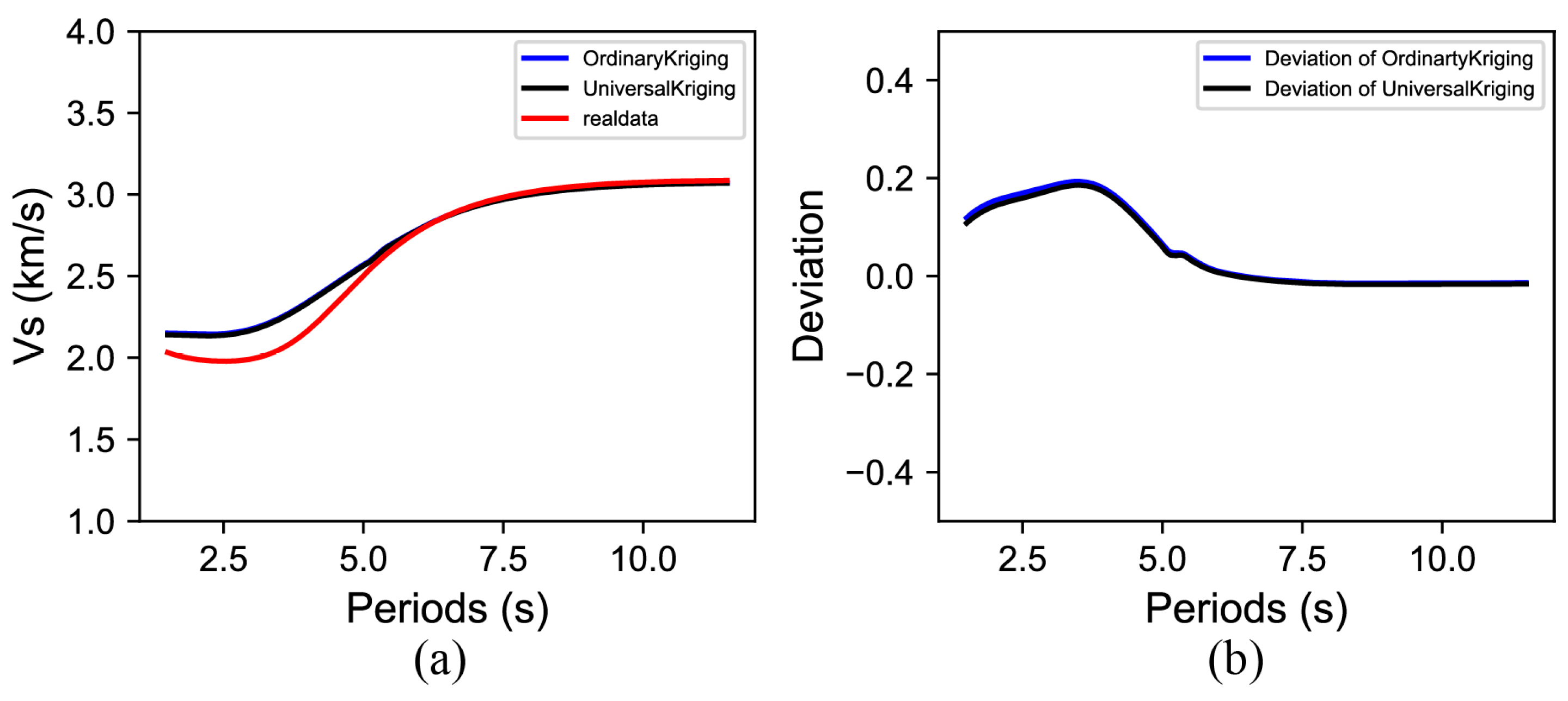
The results of the first test are shown in Figure A1, Figure A2, Figure A3, Figure A4, Figure A5, Figure A6, Figure A7, Figure A8 and Figure A9. The lost point was due to the distance and deviation angle limitations mentioned in Section 3.2. The RMSE was calculated to be 0.06. The max errors were 3% for OK and 4.6% for UK (relative error in Figure 5), which can be considered acceptable [37]. Therefore, we believe that interpolating dispersion curves using kriging is feasible, and this method can be used to obtain an accurate dispersion curve. In addition, combined with the RMSE of the remaining tests mentioned in Section 4.1, the results will be more accurate if we have more input data. It is worth noting that the red lines in Figure A1, Figure A2, Figure A3, Figure A4, Figure A5, Figure A6, Figure A7, Figure A8 and Figure A9 have similar shapes. This shows that the method works well for models where the VS structure is not complex.
According to Figure 6, the deviation of the dispersion curves interpolated by UK was less than with OK. This is because ordinary kriging requires that the regionalized variable Z(x) be second-order stationary (i.e., E[Z(x)] is a constant); however, the composition of the material in the earth’s crust is complex, and some of the material in the volcanic area comes from deeper. Therefore, UK is more suitable for volcanic areas than OK. The results shown in Figure A10, Figure A11, Figure A12 and Figure A13 prove that the results were not casual, so we chose UK as the ‘method’ parameter for interpolation.
The third test is the sensitivity test about the parameters proposed in Section 3.2. The results demonstrate how the distance (search scope) influences the interpolation accuracy (Figure 7a–d). Figure 7a–d represent the RMSE of the interpolated results with search scopes of 10,000 m, 15,000 m, 20,000 m, and 30,000 m, respectively. Moreover, the mean of each RMSE is shown in the top right-hand corner. The larger the search scope, the higher the time cost; however, it is not necessary to obtain more accurate results. According to Table A2, “angle” hardly affects the accuracy of the interpolation, because “angle” is proposed to limit the range of interpolation, and “distance” mainly determines the amount of data participating in the interpolation. There is no real data to be compared with the predicted outside the array. If not restricted, the predicted results are meaningless. When “angle” is set larger, more predicted results are obtained, and more results are unacceptable. Therefore, “distance” is set to be 15,000 m, and “angle” is set to be 265° in this study.
In the application of the interpolation method, different depths have different expansion multiples (Table 3). This is because different original dispersion curves have different period ranges. There are few original data in the long periods (e.g., larger than 10 s). Comparing Figure 4a–c and Figure 4d–f, the interpolation results with grid translation (Figure 4a–c) were very similar to the original results (Figure 4d–f), which provides evidence of the feasibility of dispersion curve interpolation using kriging.
For the changes in the depth (e.g., 15 km), on the one hand, direct inversion will obtain more detailed information about areas with high ray density. The results obtained by inverting the predicted dispersion curves will be affected by the forward process and the interpolation process, which makes the results in the depth (e.g., 15 km) smooth. The image with interpolated data is helpful for portraying large anomalies. On the other hand, due to the small number of long-period dispersion data, the structure in the deep is not well restrained. Through the forward process and interpolation process, more long-period data are obtained, which makes restriction in the deep work better.
There is no denying that there are some limitations of the dispersion curve interpolation. The accuracy of the predicted dispersion in different periods is not the same, which may affect the precision of inversion. The original data in this study is evenly distributed in the study area. If the data is unevenly distributed, the predicted results will be impacted.
6. Conclusions
In this study, we developed a process of dispersion curve interpolation based on kriging, and proved the applicability of the process through several different tests. This study provides a basis for subsequent temporal–spatial interpolation of dispersion curves. The mean RMSE of the predicted data is less than 0.1 and the max relative error is less than 10%. Moreover, the interpolation method provides new ways for the data supplementation of noise source imaging. Cross-validation is used to determine the best variogram in this study. According to the sensitivity analysis, “distance” and “angle” are determined to be 15,000 m and 265° in this study. If the method is used in a different data set, the parameters should be reset. Finally, the method is applied in the Changbai volcano, which complements the areas with low ray density and expands the original imaging area. The max expansion multiple can reach 2.4. The application of the method can reduce the cost of field work.
Author Contributions
Conceptualization, Y.T. and P.Z.; methodology, H.Z., Y.T. and P.Z.; software, H.Z.; validation, H.Z.; formal analysis, H.Z., Y.T. and P.Z.; investigation, H.Z.; resources, Y.T. and P.Z.; data curation, H.Z. and Y.T.; writing—original draft preparation, H.Z.; writing—review and editing, P.Z.; visualization, H.Z.; funding acquisition, Y.T. All authors have read and agreed to the published version of the manuscript.
Funding
This study was funded by the National Natural Science Foundation of China (grant No. 42274065), the National Key R&D Program of China (Grant No. 2022YFF0801003), the Program for JLU Science and Technology Innovative Research Team (No. 2021TD-05) and Fundamental Research Funds for the Central Universities in China.
Institutional Review Board Statement
Not applicable.
Informed Consent Statement
Not applicable.
Data Availability Statement
The Vs model of the Changbai volcano (Changbai model) is available at the https://doi.org/10.5281/zenodo.7509119 (accessed on 6 January 2023).
Acknowledgments
We thank Qingjun Kong and Chengzhi Wu of the Changbaishan Volcano Observatory for their help in the fieldwork. We thank Dong Yan, Zhiqiang Li and Jie Li for their work in the Changbai volcano. We also appreciate Weiming Wu for his help in this study. We thank the editor and four referees for their comments and efforts to improve the manuscript.
Conflicts of Interest
The authors declare no conflict of interest.
Appendix A

Table A1.
R–square of each variogram with different kriging in each period.
| Period (s) | Method | Variogram | R–Square |
|---|---|---|---|
| 2 | Ordinary Kriging | linear | −0.17239 |
| gaussian | 0.32272 | ||
| spherical | 0.04819 | ||
| Universal Kriging | linear | −0.20511 | |
| gaussian | −54.0814 | ||
| spherical | 0.19007 | ||
| 4 | Ordinary Kriging | linear | 0.22706 |
| gaussian | 0.24714 | ||
| spherical | 0.44061 | ||
| Universal Kriging | linear | −0.13863 | |
| gaussian | −0.07201 | ||
| spherical | 0.48276 | ||
| 6 | Ordinary Kriging | linear | 0.21364 |
| gaussian | 0.28400 | ||
| spherical | 0.35176 | ||
| Universal Kriging | linear | −0.24132 | |
| gaussian | −0.13955 | ||
| spherical | 0.28400 | ||
| 8 | Ordinary Kriging | linear | −0.01302 |
| gaussian | 0.22846 | ||
| spherical | 0.27741 | ||
| Universal Kriging | linear | −0.63261 | |
| gaussian | −363.477 | ||
| spherical | 0.27772 | ||
| 10 | Ordinary Kriging | linear | −0.34288 |
| gaussian | 0.32577 | ||
| spherical | 0.14228 | ||
| Universal Kriging | linear | −0.90197 | |
| gaussian | −655.004 | ||
| spherical | 0.20754 |
Table A2.
Sensitivity test.
| 185° | 230° | 265° | 300° | |
|---|---|---|---|---|
| 10,000 m | 0.140 | 0.140 | 0.139 | 0.145 |
| 15,000 m | 0.075 | 0.075 | 0.076 | 0.0797 |
| 20,000 m | 0.079 | 0.079 | 0.080 | 0.0830 |
| 30,000 m | 0.093 | 0.093 | 0.095 | 0.1000 |
Figure A1.
Comparison of dispersion curve interpolation results (127.76° E, 42.06° N). The blue curve indicates the ordinary kriging results, while the black curve indicates those of universal kriging: (a) Comparison of dispersion curves; and (b) deviation of the OK (blue) or UK (black) results.
Figure A1.
Comparison of dispersion curve interpolation results (127.76° E, 42.06° N). The blue curve indicates the ordinary kriging results, while the black curve indicates those of universal kriging: (a) Comparison of dispersion curves; and (b) deviation of the OK (blue) or UK (black) results.
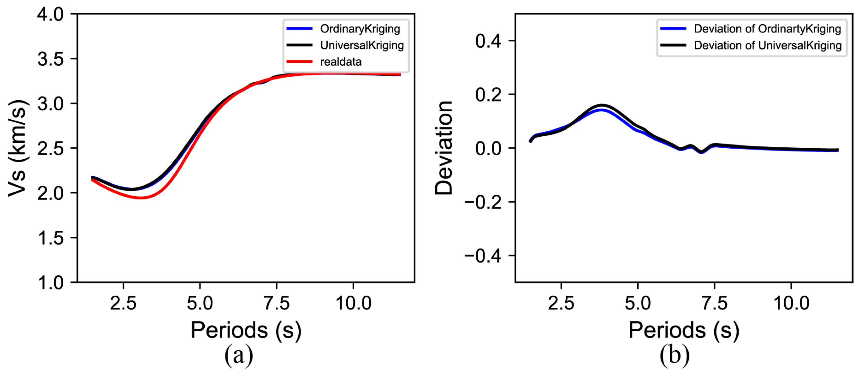
Figure A2.
Comparison of dispersion curve interpolation results (127.91° E, 41.94° N). The blue curve indicates the ordinary kriging results, while the black curve indicates those of universal kriging: (a) Comparison of the dispersion curves; and (b) deviation of the OK (blue) or UK (black) results.

Figure A3.
Comparison of dispersion curve interpolation results (128.0° E, 42.0° N). The blue curve indicates the ordinary kriging results, while the black curve indicates those of universal kriging: (a) Comparison of the dispersion curves; and (b) deviation of the OK (blue) or UK (black) results.
Figure A3.
Comparison of dispersion curve interpolation results (128.0° E, 42.0° N). The blue curve indicates the ordinary kriging results, while the black curve indicates those of universal kriging: (a) Comparison of the dispersion curves; and (b) deviation of the OK (blue) or UK (black) results.
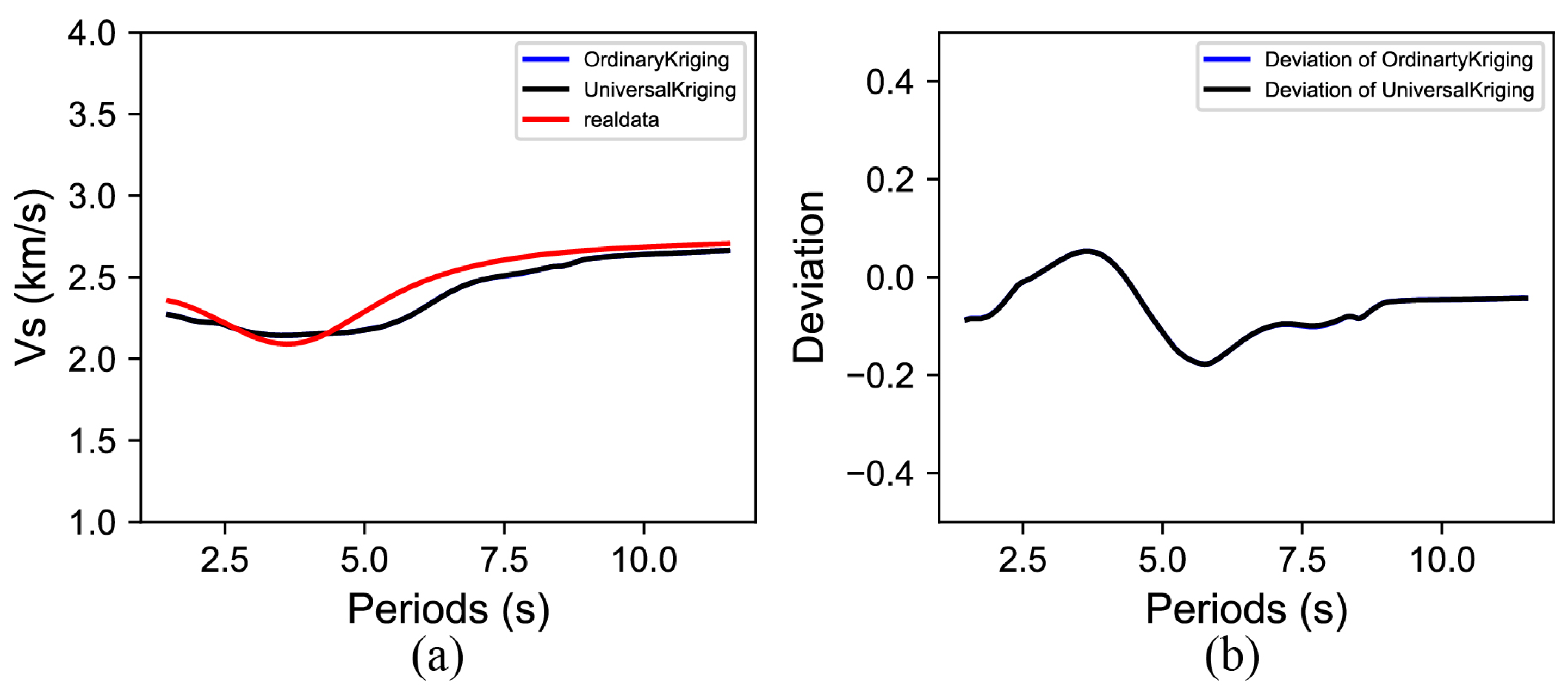
Figure A4.
Comparison of dispersion curve interpolation results (128.09° E, 41.88° N). The blue curve indicates the ordinary kriging results, while the black curve indicates those of universal kriging: (a) Comparison of the dispersion curves; and (b) deviation of the OK (blue) or UK (black) results.

Figure A5.
Comparison of dispersion curve interpolation results (128.18° E, 41.76° N). The blue curve indicates the ordinary kriging results, while the black curve indicates those of universal kriging: (a) Comparison of the dispersion curves; and (b) deviation of the OK (blue) or UK (black) results.

Figure A6.
Comparison of dispersion curve interpolation results (128.18° E, 41.82° N). The blue curve indicates the ordinary kriging results, while the black curve indicates those of universal kriging: (a) Comparison of the dispersion curves; and (b) deviation of the OK (blue) or UK (black) results.

Figure A7.
Comparison of dispersion curve interpolation results (128.18° E, 42.18° N). The blue curve indicates the ordinary kriging results, while the black curve indicates those of universal kriging: (a) Comparison of the dispersion curves; and (b) deviation of the OK (blue) or UK (black) results.
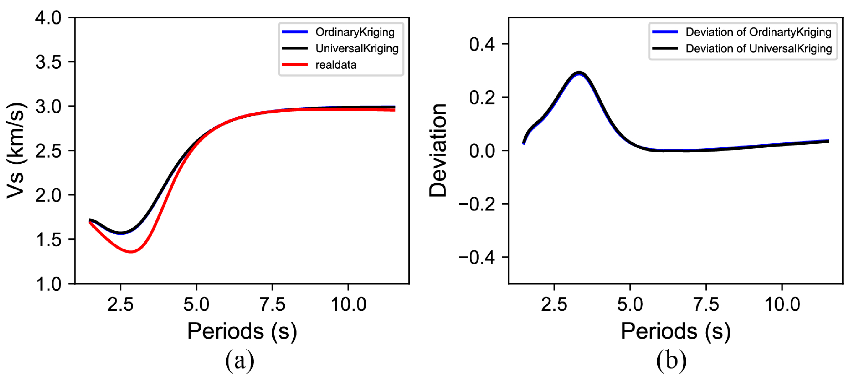
Figure A8.
Comparison of dispersion curve interpolation results (128.18° E, 42.27° N). The blue curve indicates the ordinary kriging results, while the black curve indicates those of universal kriging: (a) Comparison of the dispersion curves; and (b) deviation of the OK (blue) or UK (black) results.
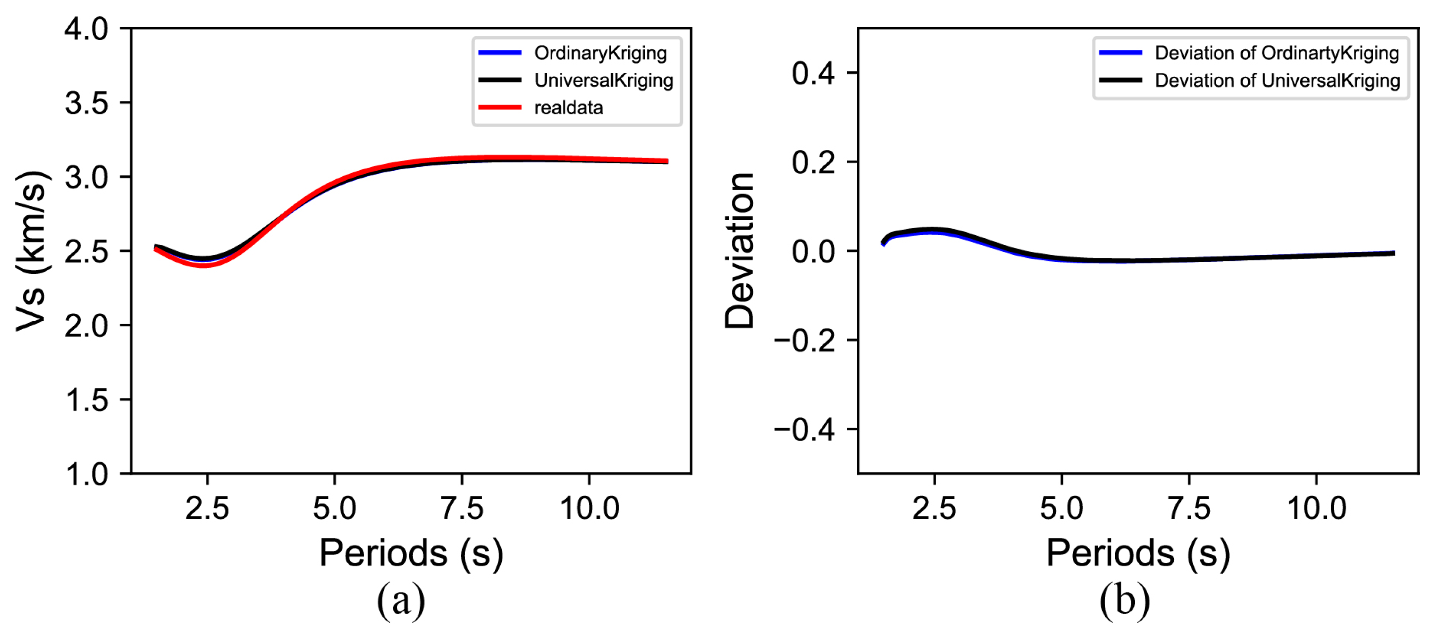
Figure A9.
Comparison of dispersion curve interpolation results (128.21° E, 42.24° N). The blue curve indicates the ordinary kriging results, while the black curve indicates those of universal kriging: (a) Comparison of the dispersion curves; and (b) deviation of the OK (blue) or UK (black) results.
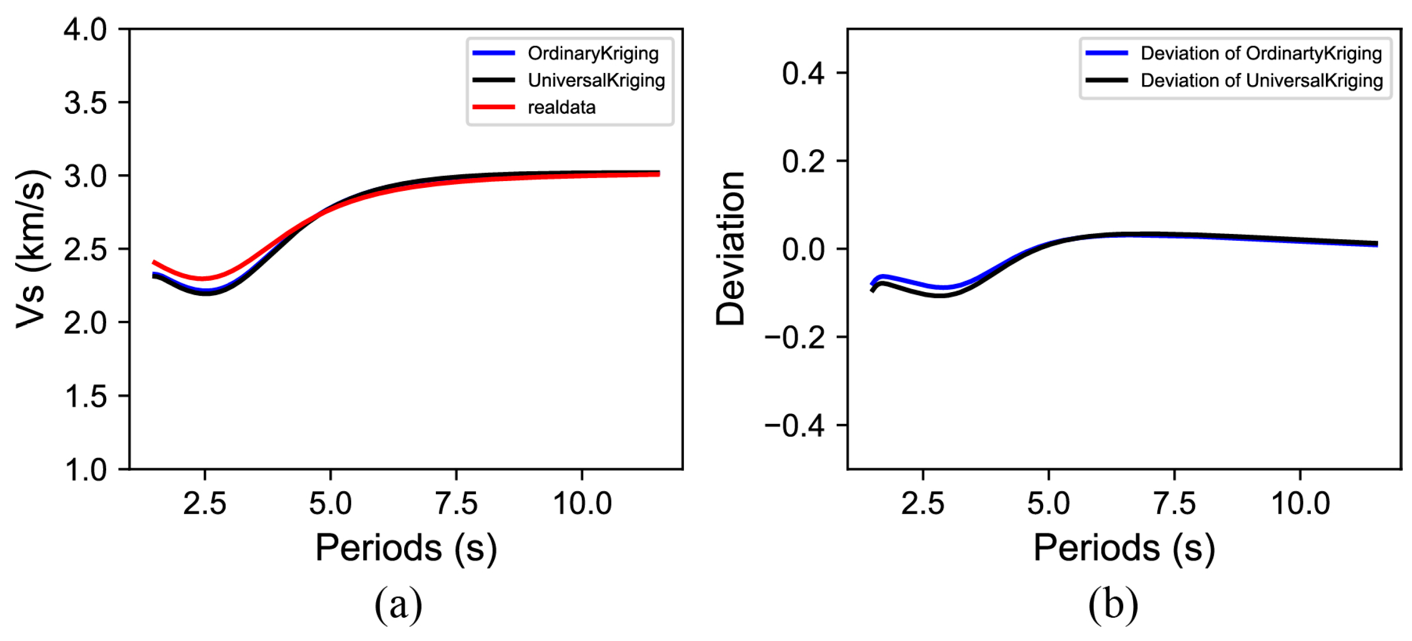
Figure A10.
An additional test to compare the RMSE of different methods: (a) OK; and (b) UK. The mean RMSEs and parameters are listed in the top right-hand corner.
Figure A10.
An additional test to compare the RMSE of different methods: (a) OK; and (b) UK. The mean RMSEs and parameters are listed in the top right-hand corner.
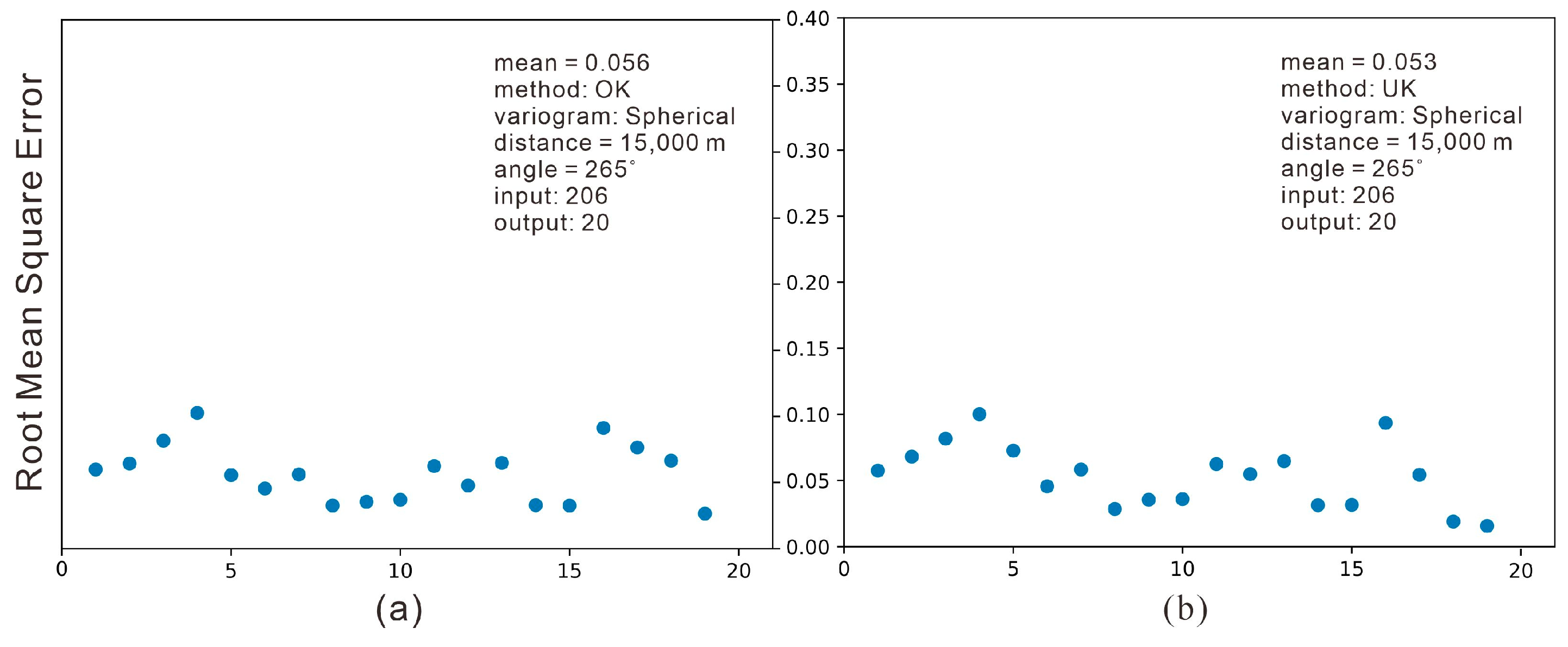
Figure A11.
An additional test to compare the RMSE of different methods: (a) OK; and (b) UK. The mean RMSEs and parameters are listed in the top right-hand corner.
Figure A11.
An additional test to compare the RMSE of different methods: (a) OK; and (b) UK. The mean RMSEs and parameters are listed in the top right-hand corner.
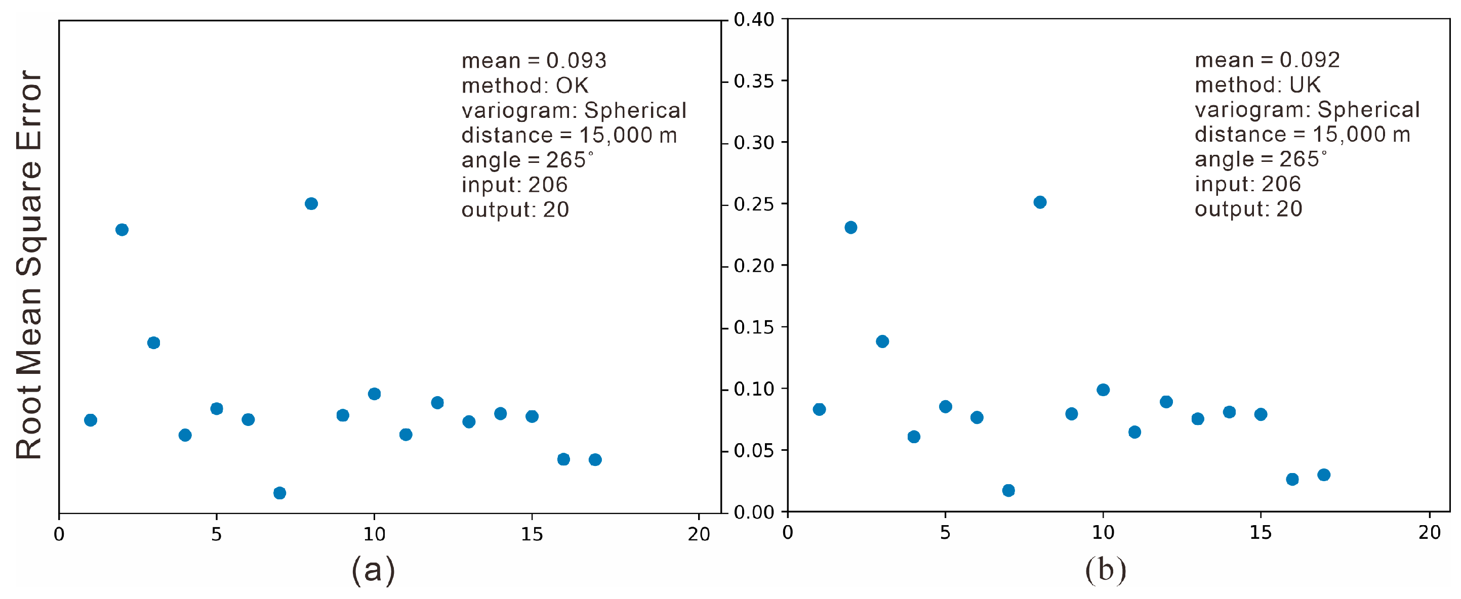
Figure A12.
An additional test to compare the RMSE of different methods: (a) OK; and (b) UK. The mean RMSEs and parameters are listed in the top right-hand corner.
Figure A12.
An additional test to compare the RMSE of different methods: (a) OK; and (b) UK. The mean RMSEs and parameters are listed in the top right-hand corner.
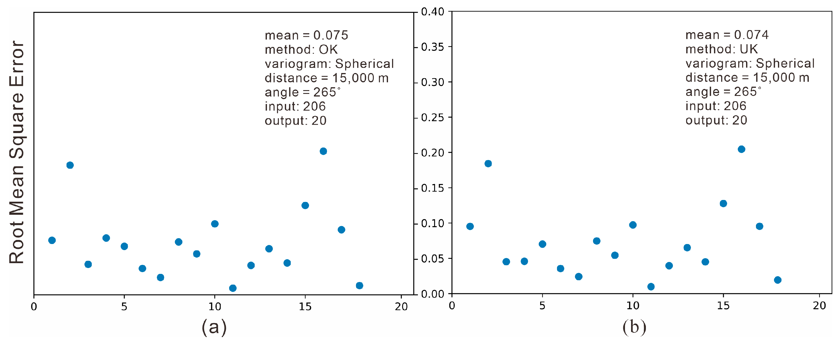
Figure A13.
An additional test to compare the RMSE of different methods: (a) OK; and (b) UK. The mean RMSEs and parameters are listed in the top right-hand corner.
Figure A13.
An additional test to compare the RMSE of different methods: (a) OK; and (b) UK. The mean RMSEs and parameters are listed in the top right-hand corner.
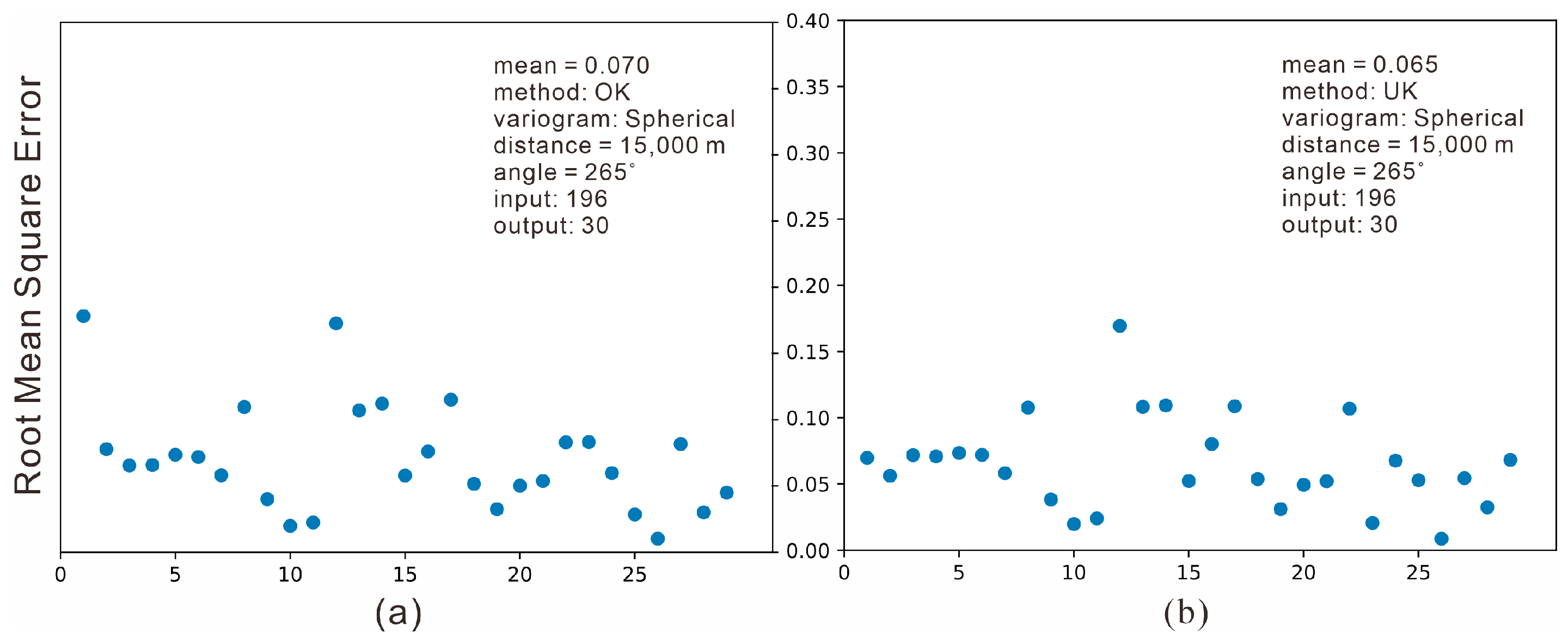
Figure A14.
Combination of the interpolation and original results with 0.01° × 0.01° grid.

Figure A15.
Original results imaged by 0.01° × 0.01° grid at different depths.

References
- Hutapea, F.L.; Tsuji, T.; Ikeda, T. Real-time crustal monitoring system of Japanese Islands based on spatio-temporal seismic velocity variation. Earth Planets Space 2020, 72, 19. [Google Scholar] [CrossRef]
- Li, L.; Revesz, P. Interpolation methods for spatio-temporal geographic data. Comput. Environ. Urban Syst. 2004, 28, 201–227. [Google Scholar] [CrossRef]
- Antonić, O.; Križan, J.; Marki, A.; Bukovec, D. Spatio-temporal interpolation of climatic variables over large region of complex terrain using neural networks. Ecol. Model. 2001, 138, 255–263. [Google Scholar] [CrossRef]
- Kilibarda, M.; Tadić, M.P.; Hengl, T.; Luković, J.; Bajat, B. Global geographic and feature space coverage of temperature data in the context of spatio-temporal interpolation. Spat. Stat. 2015, 14, 22–38. [Google Scholar] [CrossRef]
- Li, S.; Griffith, D.A.; Shu, H. Temperature prediction based on a space-time regression-kriging model. J. Appl. Stat. 2020, 47, 1168–1190. [Google Scholar] [CrossRef]
- Bezyk, Y.; Sówka, I.; Górka, M.; Blachowski, J. Gis-based approach to spatio-temporal interpolation of atmospheric co2 concentrations in limited monitoring dataset. Atmosphere 2021, 12, 384. [Google Scholar] [CrossRef]
- Revesz, P. Spatiotemporal Interpolation Algorithms. In Encyclopedia of Database Systems; Liu, L., Özsu, M.T., Eds.; Springer: Boston, MA, USA, 2009; pp. 2736–2739. [Google Scholar]
- Shapiro, N.M.; Campillo, M.; Stehly, L.; Ritzwoller, M.H. High-Resolution Surface-Wave Tomography from Ambient Seismic Noise. Science 2005, 307, 1615–1618. [Google Scholar] [CrossRef] [Green Version]
- Lin, F.-C.; Ritzwoller, M.H.; Townend, J.; Bannister, S.; Savage, M.K. Ambient noise Rayleigh wave tomography of New Zealand. Geophys. J. Int. 2007, 170, 649–666. [Google Scholar] [CrossRef] [Green Version]
- Yang, Y.; Ritzwoller, M.H.; Levshin, A.L.; Shapiro, N.M. Ambient noise Rayleigh wave tomography across Europe. Geophys. J. Int. 2007, 168, 259–274. [Google Scholar] [CrossRef] [Green Version]
- Shen, W.; Ritzwoller, M.H.; Kang, D.; Kim, Y.; Lin, F.-C.; Ning, J.; Wang, W.; Zheng, Y.; Zhou, L. A seismic reference model for the crust and uppermost mantle beneath China from surface wave dispersion. Geophys. J. Int. 2016, 206, 954–979. [Google Scholar] [CrossRef] [Green Version]
- Zhu, H.; Tian, Y.; Zhao, D.; Li, H.; Liu, C. Seismic Structure of the Changbai Intraplate Volcano in NE China From Joint Inversion of Ambient Noise and Receiver Functions. J. Geophys. Res. Solid Earth 2019, 124, 4984–5002. [Google Scholar] [CrossRef] [Green Version]
- Li, Z.; Ni, S.; Zhang, B.; Bao, F.; Zhang, S.; Deng, Y.; Yuen, D.A. Shallow magma chamber under the Wudalianchi Volcanic Field unveiled by seismic imaging with dense array. Geophys. Res. Lett. 2016, 43, 4954–4961. [Google Scholar] [CrossRef] [Green Version]
- Levshin, A.L.; Ritzwoller, M.H. Automated Detection, Extraction, and Measurement of Regional Surface Waves. Pure Appl. Geophys. 2001, 158, 1531–1545. [Google Scholar] [CrossRef]
- Natale, M.; Nunziata, C.; Panza, G.F. Average shear wave velocity models of the crustal structure at Mt. Vesuvius. Phys. Earth Planet. Int. 2005, 152, 7–21. [Google Scholar] [CrossRef]
- Wang, J.; Wu, G.; Chen, X. Frequency-Bessel Transform Method for Effective Imaging of Higher-Mode Rayleigh Dispersion Curves from Ambient Seismic Noise Data. J. Geophys. Res. Solid Earth 2019, 124, 3708–3723. [Google Scholar] [CrossRef] [Green Version]
- Wu, G.-X.; Pan, L.; Wang, J.-N.; Chen, X. Shear Velocity Inversion Using Multimodal Dispersion Curves from Ambient Seismic Noise Data of USArray Transportable Array. J. Geophys. Res. Solid Earth 2020, 125, e2019JB018213. [Google Scholar] [CrossRef]
- Li, H.; Tian, Y.; Zhao, D.; Kumar, R.; Li, H.; Yan, D.; Liu, C. Shear-wave tomography of the Changbai volcanic area in NE China derived from ambient noise and seismic surface waves. J. Asian Earth Sci. 2022; in press. [Google Scholar] [CrossRef]
- Fang, H.; Yao, H.; Zhang, H.; Huang, Y.-C.; van der Hilst, R.D. Direct inversion of surface wave dispersion for three-dimensional shallow crustal structure based on ray tracing: Methodology and application. Geophys. J. Int. 2015, 201, 1251–1263. [Google Scholar] [CrossRef] [Green Version]
- Chen, Y.; Chen, X.; Wang, Y.; Zu, S. The Interpolation of Sparse Geophysical Data. Surv. Geophys. 2019, 40, 73–105. [Google Scholar] [CrossRef]
- Wu, G.; Liu, Y.; Liu, C.; Zheng, Z.; Cui, Y. Seismic data interpolation using deeply supervised U-Net++ with natural seismic training sets. Geophys. Prospect. 2023, 71, 227–244. [Google Scholar] [CrossRef]
- Garabito, G. Prestack seismic data interpolation and enhancement with common-reflection-surface–based migration and demigration. Geophys. Prospect. 2021, 69, 913–925. [Google Scholar] [CrossRef]
- Krige, D.G. A statistical approach to some basic mine valuation problems on the Witwatersrand. J. S. Afr. Inst. Min. Metall. 1951, 52, 119–139. [Google Scholar] [CrossRef]
- Matheron, G. Principles of geostatistics. Econ. Geol. 1963, 58, 1246–1266. [Google Scholar] [CrossRef]
- Pereira, P.E.C.; Rabelo, M.N.; Ribeiro, C.C.; Diniz-Pinto, H.S. Geological modeling by an indicator kriging approach applied to a limestone deposit in Indiara city—Goiás. REM—Int. Eng. J. 2017, 70, 331–337. [Google Scholar] [CrossRef] [Green Version]
- Journel, A.G.; Alabert, F.G. New method for reservoir mapping. J. Pet. Technol. 1990, 42, 212–218. [Google Scholar] [CrossRef]
- Kumar, V. Optimal contour mapping of groundwater levels using universal kriging—A case study. Hydrol. Sci. J. 2007, 52, 1038–1050. [Google Scholar] [CrossRef]
- Kaur, L.; Rishi, M.S. Integrated geospatial, geostatistical, and remote-sensing approach to estimate groundwater level in north-western India. Environ. Earth Sci. 2018, 77, 786. [Google Scholar] [CrossRef]
- Chica-Olmo, M.; Luque-Espinar, J.A. Applications of the local estimation of the probability distribution function in environmental sciences by kriging methods. Inverse Probl. 2002, 18, 25–36. [Google Scholar] [CrossRef]
- Kurtulus, T.; Kurtulus, B.; Avsar, O.; Avsar, U. Evaluating the thermal stratification of Koycegiz Lake (SW Turkey) using in-situ and remote sensing observations. J. Afr. Earth Sci. 2019, 158, 103559. [Google Scholar] [CrossRef]
- Bensen, G.D.; Ritzwoller, M.H.; Barmin, M.P.; Levshin, A.L.; Lin, F.; Moschetti, M.P.; Shapiro, N.M.; Yang, Y. Processing seismic ambient noise data to obtain reliable broad-band surface wave dispersion measurements. Geophys. J. Int. 2007, 169, 1239–1260. [Google Scholar] [CrossRef] [Green Version]
- Luo, Y.; Yang, Y.; Xu, Y.; Xu, H.; Zhao, K.; Wang, K. On the limitations of interstation distances in ambient noise tomography. Geophys. J. Int. 2015, 201, 652–661. [Google Scholar] [CrossRef] [Green Version]
- Eric, N.N.; Charles, T.T.; Alain-Pierre, K.T. Frequency Time Analysis (FTAN) and Moment Tensor Inversion Solutions from Short Period Surface Waves in Cameroon (Central Africa). Open J. Geol. 2014, 4, 33–43. [Google Scholar] [CrossRef] [Green Version]
- Oliver, M.A.; Webster, R. A tutorial guide to geostatistics: Computing and modelling variograms and kriging. Catena 2014, 113, 56–69. [Google Scholar] [CrossRef]
- Wakefield, J. Statistical Analysis of Environmental Space-Time Processes edited by N. D. Le and J. V. Zidek. Biometrics 2007, 63, 624–625. [Google Scholar] [CrossRef]
- Kleijnen, J.P.C. Kriging metamodeling in simulation: A review. Eur. J. Oper. Res. 2009, 192, 707–716. [Google Scholar] [CrossRef] [Green Version]
- Jin, C.; Yang, W.H.; Luo, D.G.; Liu, J.P. Comparative analysis of extracting methods of surface wave dispersion curves. Prog. Geophys. 2016, 31, 2735–2742. (In Chinese) [Google Scholar] [CrossRef]
Figure 1.
The study region. The blue triangles represent the locations of seismometers. The red symbols indicate the three main craters in the region.
Figure 1.
The study region. The blue triangles represent the locations of seismometers. The red symbols indicate the three main craters in the region.
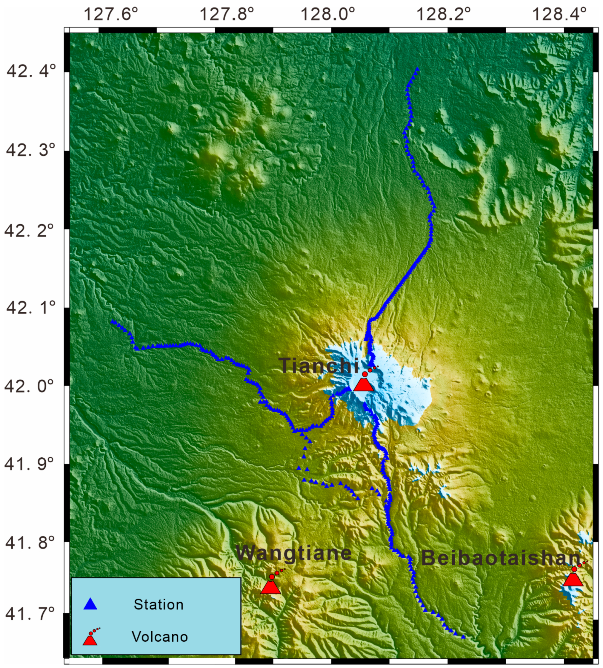
Figure 2.
The original ambient noise tomography results for different depths.

Figure 3.
Determination of the deviation angle.
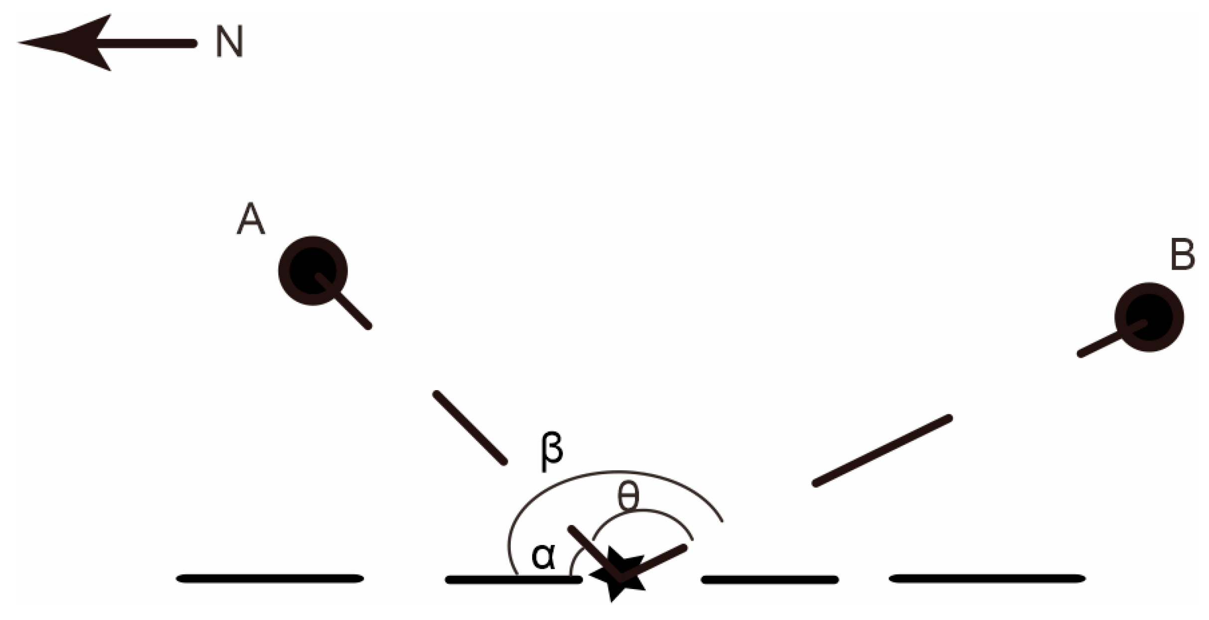
Figure 4.
Results at different depths: (a–c) Interpolated results with grid translation; (d–f) original results inverted by CPS330; and (g–i) combination of the interpolation results and the original results (inverted by CPS330).
Figure 4.
Results at different depths: (a–c) Interpolated results with grid translation; (d–f) original results inverted by CPS330; and (g–i) combination of the interpolation results and the original results (inverted by CPS330).
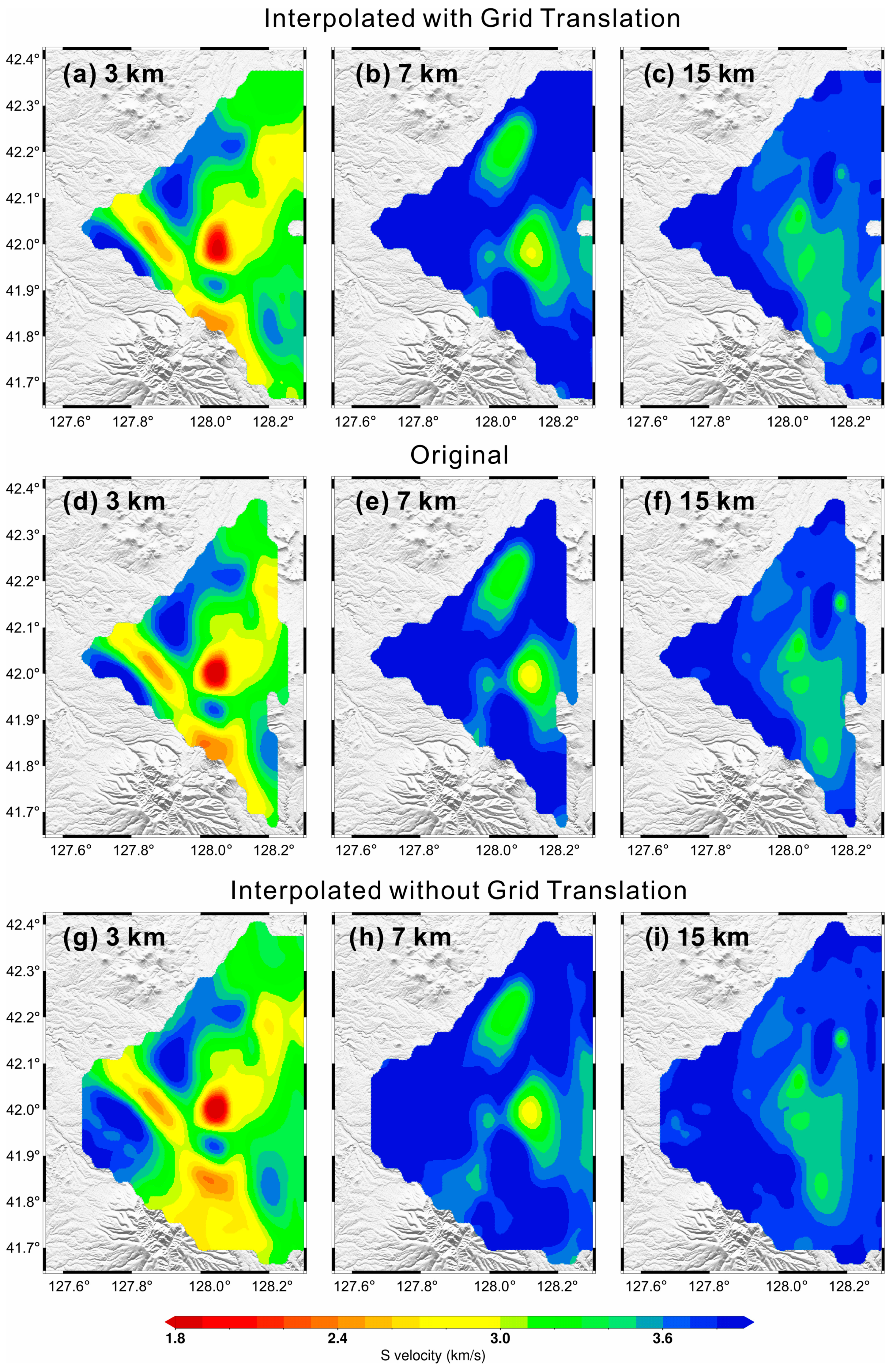
Figure 5.
Relative error of each interpolation result with different methods: (a) Relative error of the results interpolated by OK. The mean is 1.9%; and (b) Relative error of the results interpolated by UK. The mean is 2.1%.
Figure 5.
Relative error of each interpolation result with different methods: (a) Relative error of the results interpolated by OK. The mean is 1.9%; and (b) Relative error of the results interpolated by UK. The mean is 2.1%.
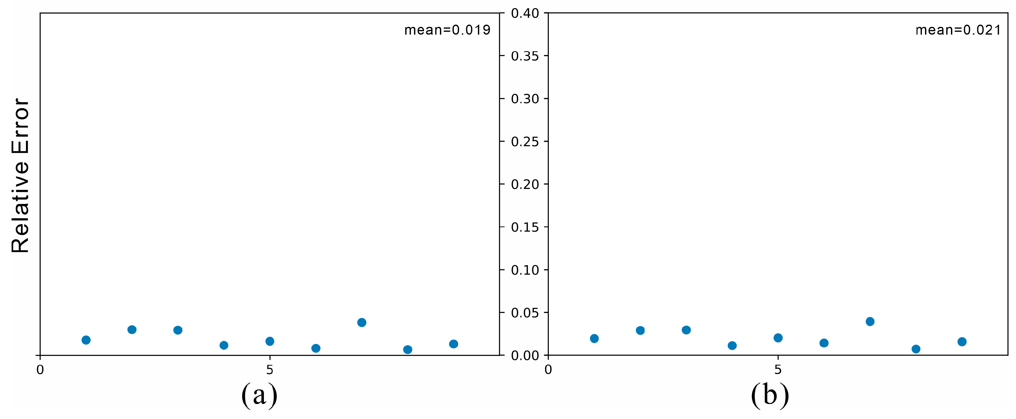
Figure 6.
RMSE of each interpolation result with different methods: (a) RMSE of the results interpolated by OK. The mean RMSE is 0.106; and (b) RMSE of the results interpolated by UK. The mean RMSE is 0.085.
Figure 6.
RMSE of each interpolation result with different methods: (a) RMSE of the results interpolated by OK. The mean RMSE is 0.106; and (b) RMSE of the results interpolated by UK. The mean RMSE is 0.085.
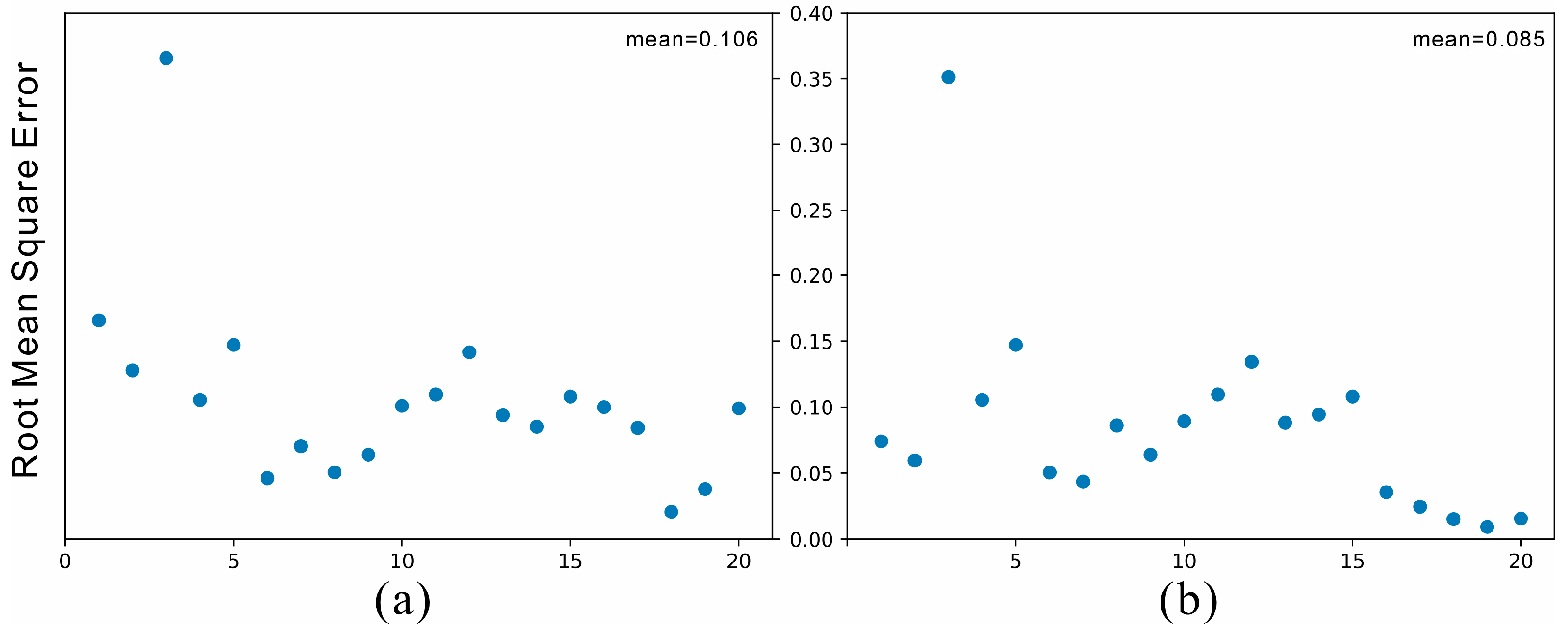
Figure 7.
RMSE of each interpolation result with different search scopes: (a) 10,000 m; (b) 15,000 m; (c) 20,000 m; and (d) 30,000 m.
Figure 7.
RMSE of each interpolation result with different search scopes: (a) 10,000 m; (b) 15,000 m; (c) 20,000 m; and (d) 30,000 m.
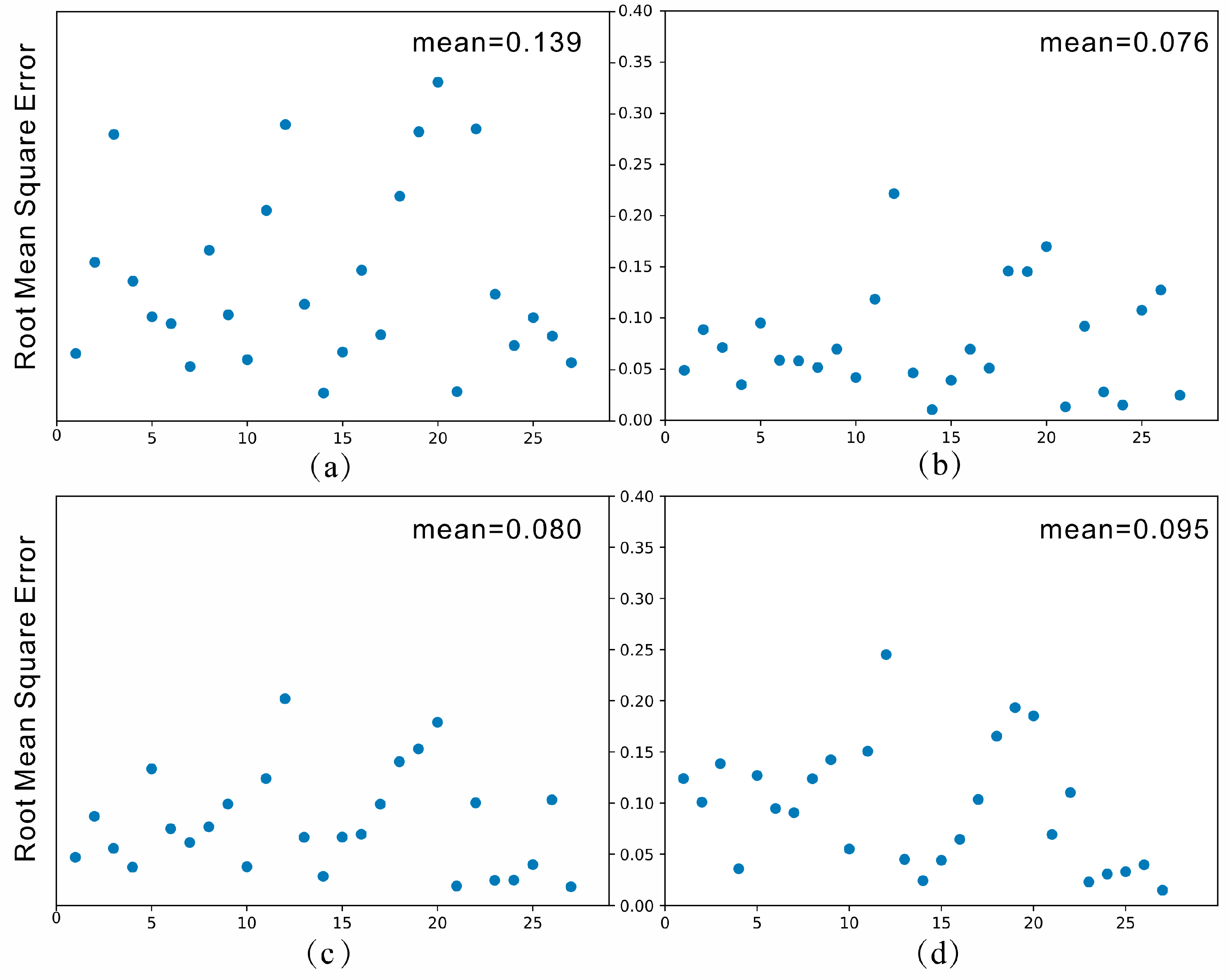
Table 1.
The best variogram under different kriging approaches in each period.
| Period (s) | Method | the Best Variogram |
|---|---|---|
| 2 | Ordinary Kriging | Gaussian |
| Universal Kriging | Spherical | |
| 4 | Ordinary Kriging | Spherical |
| Universal Kriging | Spherical | |
| 6 | Ordinary Kriging | Spherical |
| Universal Kriging | Spherical | |
| 8 | Ordinary Kriging | Spherical |
| Universal Kriging | Spherical | |
| 10 | Ordinary Kriging | Gaussian |
| Universal Kriging | Spherical |
Table 2.
Parameters used in interpolation.
| Parameter | |
|---|---|
| Method | Universal Kriging |
| Variogram | Spherical |
| Distance | 15,000 (m) |
| Angle | 265 (°) |
Table 3.
Expansion multiple at each depth.
| Depth (km) | Original | Interpolating | Expansion Multiple |
|---|---|---|---|
| 1 | 225 | 479 | 2.129 |
| 2 | 240 | 479 | 1.996 |
| 3 | 239 | 479 | 2.004 |
| 4 | 243 | 479 | 1.971 |
| 5 | 245 | 479 | 1.971 |
| 7 | 234 | 479 | 1.955 |
| 10 | 235 | 479 | 2.038 |
| 12 | 218 | 479 | 2.197 |
| 15 | 198 | 479 | 2.419 |
Disclaimer/Publisher’s Note: The statements, opinions and data contained in all publications are solely those of the individual author(s) and contributor(s) and not of MDPI and/or the editor(s). MDPI and/or the editor(s) disclaim responsibility for any injury to people or property resulting from any ideas, methods, instructions or products referred to in the content. |
© 2023 by the authors. Licensee MDPI, Basel, Switzerland. This article is an open access article distributed under the terms and conditions of the Creative Commons Attribution (CC BY) license (https://creativecommons.org/licenses/by/4.0/).
Share and Cite
MDPI and ACS Style
Zhang, H.; Tian, Y.; Zhao, P. Dispersion Curve Interpolation Based on Kriging Method. Appl. Sci. 2023, 13, 2557. https://doi.org/10.3390/app13042557
AMA Style
Zhang H, Tian Y, Zhao P. Dispersion Curve Interpolation Based on Kriging Method. Applied Sciences. 2023; 13(4):2557. https://doi.org/10.3390/app13042557
Chicago/Turabian StyleZhang, Han, You Tian, and Pengfei Zhao. 2023. "Dispersion Curve Interpolation Based on Kriging Method" Applied Sciences 13, no. 4: 2557. https://doi.org/10.3390/app13042557
Note that from the first issue of 2016, this journal uses article numbers instead of page numbers. See further details here.