

On the Regional Temperature Series Evolution in the South-Eastern Part of Romania

Department of Civil Engineering, Transilvania University of Brasov, 5, Turnului Str., 900152 Brasov, Romania
Appl. Sci. 2023, 13(6), 3904; https://doi.org/10.3390/app13063904
Submission received: 15 January 2023
/
Revised: 11 March 2023
/
Accepted: 17 March 2023
/
Published: 19 March 2023
(This article belongs to the Special Issue Regional Climate Change: Impacts and Risk Management)
Abstract
:In the context of reported climate variations in different regions of the world, this work investigates the evolution of the temperature series in the Dobrogea region, Romania, using the maximum, average, and minimum annual temperature series from 1965 to 2005. The Mann–Kendall test and Sen’s slope emphasized increasing trends of nine (out of ten) minimum temperature series (nine of them at significance levels less than or equal to 0.05, and two at 0.1), three average temperature series (at a significance level of 0.1), and five maximum temperature series (at significance levels less than or equal to 0.05). The selection of the representative series at the regional scale, called the ‘Regional series’, was performed using two algorithms proposed by the author that are easy to employ, even by individuals without deep knowledge in the field. The first (called MPPM) was initially introduced for evaluating the ‘Regional precipitation series’, and the second is a version of MPPM based on clustering the data series. Comparisons with the series from the ROCADA database were performed to prove the algorithms’ performances. The best results were obtained by running the second algorithm with two clusters, for the minimum and maximum temperature series, and with three clusters, for the average temperature series. In comparison with the initial data series, the average MAEs were, respectively, 1.39, 0.37, and 0.84 for the minimum, average, and maximum series, and the corresponding average MSEs were, respectively, 1.49, 0.41, and 0.93. Comparison of the ‘Regional series’ with the series from ROCADA led to a decrease in the modeling errors, with the best ones corresponding to the average ‘Regional series’—MAE = 0.36 and average MSE = 0.25.
1. Introduction
Performing spatial analysis of hydro-meteorological data is of central importance in water resources management for planning the water supply, irrigation, drought, and flood forecasting, as well as the mitigation of their effects at a regional scale. Owing to climate change, studies on spatial interpolation techniques are of high interest from theoretical and practical viewpoints.
Different scientists performed comparative analyses of interpolation schemes. For example, Emadia et al. [1] provided the results obtained employing four interpolation methods on monthly mean total precipitation and monthly mean air temperature, proving that in most study cases, ordinary kriging (OK) and co-kriging had the best performances evaluated by the correlation between the recorded and computed series, RMSE, and average error. Javari [2] applied eight interpolation techniques for spatial precipitation variation in Iran, while Chen and Guo [3] used spatial interpolation techniques for regionalizing climate change in Northeast China. Ozturk and Kilik [4] utilized OK for interpolating the precipitation and temperature of the Aegean Region in Turkey for different years. Wu and Li [5] employed residual kriging for the temperature interpolation, while Goovaerts [6] analyzed the performances of different multivariate methods with respect to the Thiessen Polygons Method (TPM) [7] and the inverse distance weighting method (IDW) [8]. Following the same idea, Ly, Charles, and Degre [9] and Szolgay et al. [10] proposed different variograms necessary to interpolate the daily rainfall series. Improved versions of IDW using Particle Swarm Optimization (PSO) and genetic algorithms are provided in [11,12,13].
Geostatistical methods have been developed primarily in geology, followed by applications in meteorology and forestry [14]. They have restricted use outside the structure–function (variogram). The main limitation of kriging is related to the stationarity hypothesis of data series and the necessity of large data sets for defining spatial autocorrelation [15,16]. Moreover, the stationarity in mean and variance and the existence of a Gaussian distribution are conditions that should be satisfying when employing radar and in situ data combinations [17].
Discussing what kind of spatial interpolation is adequate for meteorology, Szentimrey et al. [18] conclude that ‘the geostatistical methods cannot efficiently use the meteorological data series, whereas the data series makes possible to obtain the necessary information’ for the interpolation in meteorology. By comparison, the ‘mechanical methods’ (Thiessen polygons methods, IDW) are widely applied because they do not rely on restrictive conditions and consider the spatial and temporal aspects.
Since the existence of climatic data of high quality is necessary for assessing the climate variability in a region, gridded datasets have been created for different regions of the world [19,20,21]. The main methods utilized for this aim are data homogenization—with Multiple Analysis of Series for Homogenization (MASH) software [22]—and gridding by Meteorological Interpolation based on Surface Homogenized Data (MISH) software [23]. The gridded datasets represent a valuable input for spatially distributed hydrological agrometeorological models [19].
The interest in spatial interpolation methods resides in the practical goal of detecting the regional evolution of hydro-meteorological time series [24,25,26,27,28], especially in climate change conditions [3]. Despite their importance, many algorithms can only be performed by people with deep statistical and computational knowledge. Some methods rely on ARMA or Bayesian techniques [29,30,31,32], thin-plate smoothing splines [33], gradient-plus-inverse distance squared [34], or P-BSHADE [35,36,37]. A few are implemented in different geostatistical information systems [38,39,40], which are sometimes very hard to use, even for specialists.
In the above context, the Most Probable Precipitation Method (MPPM) was introduced [41] to estimate the regional rainfall evolution and was applied to the Dobrogea region of Romania. Comparison with TPM, OK, and IDW proved its superior performances on three sets of data series recorded at ten sites. Since MPPM works for any spatially distributed data series, a version of this algorithm was utilized to determine the aerosols’ regional tendency in the Arabian Gulf Region [42,43] and was implemented in Matlab [44].
This article assesses the regional evolution of minimum, maximum, and average temperature series in the Dobrogea region using two versions (Method I and Method II) of MPPM. Comparisons with the data series from the ROCADA database are also provided.
Moreover, by comparison with other articles that investigate only the individual temperature series evolution and the existence of an increasing/decreasing trend by the Mann–Kendall test and Sens’ slope, without advancing the regional evolution of the studied series, here, we built a representative series of the temperature evolution in Dobrogea (called ‘Regional series’), selecting values from all the series involved in the study. Other scientists did not employ this type of approach.
This attempt is also important for the following reasons:
- To evaluate the variability of the temperature series in the region.
- When applying the proposed methods, one determines the regional trend of the data series. If the available set of time series (recorded at different locations) is homogenous, and one wants to evaluate the series value at a point where it is unknown, this value can be chosen to be equal to that of the regional trend in the studied period.
2. Methodology and Data Series
2.1. Methodology
Figure 1 presents the flowchart of this study.
Two statistical tests were performed on the data series. The first one was the Mann–Kendall trend test [45] that permits testing the null hypothesis of no monotonic trend, H0, against the alternative hypothesis, H1, that there is an increasing or decreasing monotonic trend of the temperature series. Sen’s nonparametric procedure [46] was used to estimate the slope of such a trend (if it exists). The second test was that of Kruskal and Wallis [47], whose null hypothesis is that the distribution functions from which the samples are extracted are the same. In this case, the samples were the temperature series recorded at each site.
Given k data series, each of them formed by m elements, let X = (xji) (j = 1, …, m, i = 1, …, k) the matrix whose columns are the series elements (column 1—the elements of series 1, …, column k—the elements of the series k). For determining the spatial trend, the series are recorded at the same time.
MPPM has the following stages [41]:
- For each row j of X (j = 1, …, m), compute the difference between the maximum and the minimum values, call it amplitude, and denote it as Aj.
- For each j (j = 1, …, m), divide the interval between the minimum and maximum values on row j in nj intervals of the same length that contain enough values. The number of intervals, nj, is chosen based on the user experience and/or a number of trials.
- For each j (j = 1, …, m), choose the interval with the highest number of elements (call this number frequency) among those formed in the previous step. Denote this interval by Ijmax and its number of elements fjmax.
- Build the ‘Regional series’ whose values are the mean of the elements in all Ijmax.
- Represent the chart of the ‘Regional series’ in Cartesian coordinates, where the Ox is the time axis and Oy is the axis containing the values of the ‘Regional series.’
- Estimate the goodness of fit by computing MAE and MSE and build their charts. The MAE and MSE are computed using the errors obtained as the differences between the recorded values (at each station) and the ‘Regional series’ values.
The following remarks on MPPM are necessary:
- At stage 2, nj is not necessarily the same for each row in the matrix. For a small number of series, it is recommended to use the same nj. The number of values in an interval depends on the number of the series. At least ten series should be considered for building the regional series, and at least two values must be contained in each interval. Three values should be the minimum for a higher number of series to avoid intervals containing only extreme values or outliers.
- If at stage 3 in MPPM there are many intervals with the maximum frequency, it is recommended to run the next steps of the algorithm for each case. The ‘Regional series’ will be that with the minimum MAE and MSE. This approach offers a better fit of the ‘Regional series’ than the original one, which only considered the interval whose average value was the closest to the average value of the data recorded at a specific moment. We name MPPM with this improvement, Method I.
To run Method I, Climate Analyser, implemented in Matlab [44], was utilized. It involves the following stages:
- Compute_Amplitude step: compute the extreme values for each year and then the amplitude.
- Amplitude Representation step: draw the chart of amplitude.
- Compute the regional series: for each year, choose the number of intervals, compute the number of elements in each interval, select the interval with the highest number of elements, and compute the average of the elements in this interval.
- Collect the results in the Data Processing from Matlab destination tables (containing MAE and MSE).
- Draw the charts of ‘Regional series’, MAE, and MSE.
- Export to file: the modeling output is exported to the xlsx. files.
Method II has the following steps [42]:
- A.
- Set the number of clusters, n, for clustering the recorded series set.
- B.
- Select the cluster that contains the lowest number of time series, determine the columns in the matrix X containing the values of these series, and remove them from X. Denote by Xc the new matrix.
- C.
- Compute the average value of the elements in each row of the matrix Xc. Denote by the average of the elements in the row j of Xc.
- D.
- Build the ‘Regional series’ with the values from the previous step.
- E.
- Represent the ‘Regional series’ chart in Cartesian coordinates, where Ox is the time axis and Oy contains the values of the ‘Regional series’.
- F.
- Estimate the goodness of fit by computing MAE and MSE as in MPPM and draw the MAE and MSE charts (as time series).
Some remarks on Method II are necessary.
- If two clusters contain the same number, the cluster with the best separation property is selected.
- In [34], the k-means algorithm was utilized in Method II for clustering. Agglomerative hierarchical clustering was used in this study.
- In the agglomerative clustering, each cluster is initially formed by a point (in this case, a station). At the next stage, the dissimilarity between every pair of points is computed using a distance (Euclidean, here). Then, the linking criterion to merge different clusters is determined. The single, complete, average, and Ward criteria were used in our experiments. The next stage, the best clustering was chosen on the basis of the value of the agglomerative coefficient [48]. Since the closer the agglomerative coefficient to is 1, the better the clustering, the Ward method was selected among the four mentioned criteria. The process continues until all the objects are linked together. The last step is choosing the cut-off value to acquire the number of clusters [49].
- We chose to apply the hierarchical clustering for the following reasons [50]:
- a.
- In the k-means algorithm, the number of clusters, k, must be specified in advance. In the hierarchical clustering it must not be pre-specified.
- b.
- In k-means, since the k is randomly chosen, the resulting clusters may differ, whereas in the hierarchical clustering, they are always the same.
- c.
- The k-means method assigns records to each cluster for finding disjunct clusters of spherical shape on the basis of distance. Hierarchical clustering easily handles any similarity forms or distance. It was shows that when using Euclidean distance (as in the case of modeling meteorological data), hierarchical clustering outperforms the k-means algorithm.
- d.
- Hierarchical clustering can be applied to any type of attributes.
- Choosing the optimum number of clusters, n, is an optimization problem. Since the choice of n is essential for performing Method II, 30 methods were run (among which Scott [51], Mariott [52], Hubert [53], Friedmann [54], silhouette [55], gap [56]) using the NbClust package in R [57] to determine the optimum number of clusters. For example, if 14 methods indicated n = 2, 10 methods indicated n = 3, and 6 gave n = 4, on the basis of the majority principle, the optimal number of clusters was selected to be 2, followed by 3. Therefore, to compare the outputs of the two methods, the first was run with two and three intervals, and the second with two and three clusters. Worked examples for both methods are presented in [41,42].
Applying Method II involves the following steps:
- Use the NbClust package in R to determine the number of clusters.
- Use the dplyr package in R to determine the clusters.
- Select the cluster with the highest number of elements. With the series from this cluster, build a matrix Xc.
- Compute the ‘Regional series’ whose elements are the averages from each line of Xc
- Compute MAE and MSE and export the result as an xlsx. file.
To compare the methods’ outputs, the series from the previous step are imported in Matlab. Then, the ‘Regional series’, MAEs, MSEs, minimum, maximum, and amplitudes series are drawn. For comparisons of the results of one method with different numbers of intervals/clusters, the algorithm is run twice, and data are stored and then represented on the same chart.
2.2. The Studied Region and the Data Series
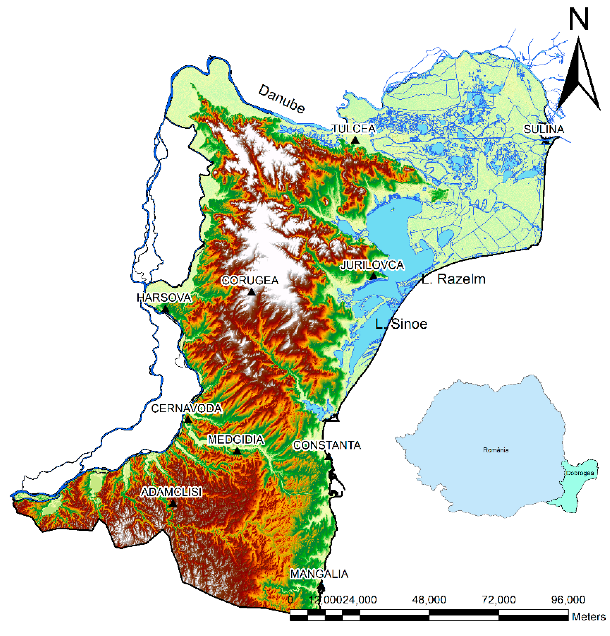
The data used for modeling consisted of annual temperatures series (minimum, maximum, and average) recorded from 1965 to 2005 at ten sites from Dobrogea, a region located in the southeast of Romania, between the lower Danube River, the Danube Delta, and the Black Sea Littoral (Figure 2), strongly influenced by the marine circulation.
The study of the average annual temperature at these meteorological stations showed an increase of 0.8 °C in annual mean temperature after 1997 [60,61]. In the same area, at Techirghiol, a dependence between the augmentation of the air temperature and that of the water has been found [62,63]. An extended study on daily average precipitation and temperature evolution using 24 indicators is presented in [64]. It was found that 1997 is a change point for the annual average temperature at all the study sites. ARIMA and GEP models for nine temperature series (two monthly and seven annual) recorded in the Dobrogea’s were also built [65].
The data series were introduced in an Excel file, each column containing the values registered at a location. The series set does not have missing values. The series whose names and locations are given in Figure 2 are denoted with consecutive numbers assigned alphabetically, from 1—Adamclisi to 10—Tulcea. The National Institute of Meteorology and Hydrology of Romania provided the data.
Figure 2.
Dobrogea and the meteorological stations [67].
Figure 2.
Dobrogea and the meteorological stations [67].
3. Results and Discussion
The minimum, mean, and maximum annual series computed as the average of the annual series recorded at the ten stations are presented in Figure 3. The series values vary in the intervals [4.8, 8.53], [9.72, 12.29], and [14.94, 17.43] for the minimum, mean, and maximum annual series, respectively. The average minimum series significantly increased after 1988: 0.6 °C—Adamclisi; 0.7 °C—Sulina and Tulcea; 0.8 °C—Constanta, Mangalia, and Medgidia; 1.1 °C—Jurilovca; 1.4 °C—Corugea; 1.5 °C—Cernavoda and Harsova.
The results of the Mann–Kendall trend test for the data series are presented in Table 1. The following symbols are used: *** if the trend is significant at the α = 0.001 level of significance, ** when it is significant at the α = 0.01 level of significance, * if the trend is significant at the α = 0.05 level of significance, and + if the trend is significant at the α = 0.1 level of significance. A blank cell means that the significance level is greater than 0.1. Q is the slope and B is the intercept computed by Sen’s procedure. At a significance level less than or equal to 0.05, H0 was rejected for eight minimum temperature series (so the existence of an increasing trend could not be rejected since Q > 0).
For the Sulina and Adamclisi minimum series, the trend existence was unable to be rejected at a significance level of 0.1. The null hypothesis was unable to be rejected for the Tulcea minimum series. Only for Constanta, Medgidia, and Mangalia average temperature series was the trend significant at a confidence level of 0.05. Out of ten maximum temperature series, four trends were significant at 0.001 (Cernavoda, Corugea, Harsova, and Jurilovca) and one at 0.01 (Jurilovca). The Kruskal–Wallis test was unable to reject the null hypothesis for the minimum, average, and maximum temperature series sets, and thus the series homogeneity was unable to be rejected.
The temperatures varied in Dobrogea during 1961–2013 as follows: the minimum between 5.6 °C and 8.4 °C, the average from 10.1 °C to 11.8 °C, and the maximum in the interval [13.1, 15.5] (°C) in the northern part and 15.7 °C–17.7 °C in the rest [19]. Despite the analysis of individual series trends, the existence of a trend over the region was not tested because the Mann–Kendall test does not have this capability and no other test has been developed for this aim.
3.1. Results and Discussion for the Minimum Temperatures Series
Figure 4 and Figure 5 shows the output of Methods I and II: (a) ‘Regional series’, (b) MAE and MSE from Method I and (c) Method II, (d) comparison of MAEs from both methods, (e) comparisons of MSEs from the methods, (f) minimum, maximum values, and the amplitude. In Figure 4a and Figure 5a, ‘Avg.’ denotes the series built of the averages of the minimum values of the series recorded during a specific year at all the sites. Method I (II) is the abbreviations for the ‘Regional series’ fitted by Method I (II).
The underestimation of the average minimum temperature at the end of the study interval in the mentioned figures shows that the average series was not a good indicator of regional series evolution [68].
Table 2 and Figure 6 contain the comparative modeling results for the minimum temperature series. In Method I, when n = 2, the MAEs and MSEs were smaller in six cases than when n = 3 intervals. The average MAE (MSE) in Method I with n = 2 was smaller than the average MAE (MSE) in the same method with n = 3 with 0.14 = 1.58−1.44 (0.07 = 1.85−1.78).
If n = 2 in Method II, MAEs (MSEs) were smaller in seven (7) cases than when n = 3. For n = 2, the average MAE (MSE) was 1.158 = 1.61/1.39 (1.18 = 1.77/1.50) times smaller than when n = 3 (Table 2). Therefore, the selection of the optimum n is important for minimizing errors. The best choice is n = 2 in this situation.
Table 2 shows that the best method for modeling the regional minimum series is Method II when using the optimal cluster number (in this case, two) because the corresponding average MAE and MSE are smaller than in Method I. Indeed, the average MAE in Method II was 1.39 (compared to the average MAE in Method I, which was 1.44), and the average MSE in Method II was 1.50 (compared to the average MSE in Method I, which was 1.78).
The highest MAEs and MSEs corresponded to the Sulina series (station 9), which had a particular position in the Danube Delta, 15 km offshore. The second highest MAEs and MSEs corresponded to the Constanta series (the third station), on the Black Sea Littoral. In this case, the differences might be derived from the data records because the station location changed during the study period.
Figure 6c,f shows significant differences among the ‘Regional series’ fitted by both methods when using two or three intervals/clusters, especially for the first 26 years. Differences of about 2 °C were noticed between the computed values by Methods I and II in the optimum case for the first 21 years. This confirms the necessity of choosing the study data set’s best segmentation (n). The differences came from the computational methodology, being related to the number of elements and the data series values involved in the computation of the ‘Regional series’. For example, if there were two clusters and the cluster with the highest number of elements has six series, then six series were involved in the computation of the ‘Regional series’. If there were three clusters, and the highest number of elements in a cluster was four, then four series were involved in the computation.
Figure 6c,f indicate periods of decreasing trends of minimum regional temperatures, followed by periods of increasing trends. It was evident that the minimum regional temperatures significantly increased after the 25th year (1990) compared to the previous period.
3.2. Results and Discussion for the Average Temperatures Series
Figure 7 and Figure 8 show the regional ‘Regional series’ obtained using Method I (II), MAE, MSE, and the amplitude for two (three) intervals/clusters for the average temperatures series. Table 2 and Figure 9 contain the comparative modeling results.
When working with two intervals/clusters, the ‘Regional series’ issued from running both algorithms appeared similar (Figure 7a). The MAE and MSE series in each method had the same pattern and comparative values (Figure 7b,c). In this case, MAEs and MSEs resulting from Method I were for five sites lower than those obtained by Method II (Figure 7e,f). The average MAE in Method I was 0.41, compared to 0.43 in Method II. MSEs were equal to 0.46 in both methods (Table 3). Therefore, for n = 2, the best results were given by Method I. The highest MAE and MSE corresponded to the fourth series (Corugea), situated in the Casimcea Plateau, at the highest altitude among the meteorological stations.
When n = 3, the ‘Regional series’ values computed by the first algorithm were generally higher than those of the similar series calculated by the second algorithm (Figure 8a). In Figure 8a, a pick of the ‘Regional series’ was emphasized in 1981. This was due to the selection of the values for building the regional series, as a result of high differences between the values recorded in 1981 to the ten meteorological stations.
MAEs (MSEs) from Method I were higher than the corresponding ones obtained in Method II (Figure 8d,e) for seven (7) sites. In this case, the best model was given by Method II. Overall, when working with average temperatures, the best model was obtained by Method II, with three clusters.
Figure 9c,f reveals high variations of the regional evolution of the average temperatures, especially after 1988, in concordance with the temperature increase in the entire region (as presented in the first paragraph of the Results and Discussion section).
3.3. Results and Discussion for the Maximum Temperatures Series
Figure 10, Figure 11 and Figure 12 display the modeling results for the maximum annual temperatures. The average series (Figure 10a and Figure 11a) had lower values than those of the ‘Regional series’ fitted by both methods, indicating that the average series did not clearly describe the evolution of the temperature series at the regional level.
For n = 2, the ‘Regional series’ (Figure 10a) had the same pattern, with lower values for Method I in the years 17, 37, and 39. There was a balance between the number of times when MAEs (MSEs) from an algorithm were greater than those from the second (five times, each) (Figure 10d,e). The average MAEs were equal, while the average MSE was slightly better in Method I.
When n = 3 (Figure 11), the ‘Regional series’ issued from the second algorithm obtained the highest values, and the average MAE (MSE) from Method I was smaller (higher) than from Method II. The algorithm produced the highest MAEs and MSEs for station 9—Sulina (Figure 10c–e and Figure 11c–e) in all cases.
Figure 12 emphasizes high variation of the ‘Regional series’, describing the regional evolution of the maximum temperatures. The numerical comparisons between the results obtained with n = 2 and n = 3 are provided in Table 4.
Generally, a slight difference between the fitted values was noticed if the two methods worked similarly. High differences appeared if one method was much better than another. The same was true when comparing the differences between the output of a single method for a different number of clusters. For example, in Figure 12f, Method II worked well in both situations (n = 2 and n = 3). A slight difference was observed in 1998–2002.
In contrast, there were significant differences between the performances of the first method when working with two and three intervals (Figure 12c), especially between 1964 and 1974. Moreover, the highest differences (with respect to MSE and MAE) were noted for the values fitted for the seventh and eighth stations (Mangalia and Medgidia). Still, the average MAEs were the same (0.84), and the average MSEs were almost equal (0.97 and 0.99, respectively) for both n = 2 and n = 3.
Both methods did not fit the data from Sulina (the ninth series) well for the reasons presented above. In this case, MAEs were between 2.23 and 2.56, and MSE between 2.32 and 2.61, by comparison to the indicators corresponding to the other stations (which were in the intervals [0.27, 1.38]—MAE, and [0.38, 1.43]—MSE).
To conclude, Method II, with n = 2, was suitable for modeling the regional evolution of maximum temperatures (the average MAE = 0.84, the average MSE = 0.93).
By comparison with the ‘Regional series’ of minimum temperatures, which recorded an augmentation in the last 24 years of the study, indicating a regional increase in the minimum temperature, the ‘Regional series’ of maximum temperatures presented high picks only in a few years (26,30, 35–38), which was in concordance with the finding from Table 1 (that indicated the absence of trend at a significance level less than 0.05 for most of the maximum series).
3.4. Comparison of the Regional Series with the Values from the ROCADA Database
Table 5 provides a comparative analysis of the best ‘Regional series’ for minimum, average, and maximum temperatures with the series from the ROCADA database. According to the previous sections, Method II performed the best. Therefore, in Table 5, MII is the abbreviation of this method with the best performances.
Since the series of interest should model the regional evolution of the temperature series, the average values were of interest (last row in Table 5). The lower the MAE and MSE, the better the model.
Generally, comparisons of the ‘Regional series’ with the series from ROCADA showed slightly lower MAEs and MSEs. The best results were obtained when working with the average temperature series. They were the average MAE = 0.36 and average MSE = 0.25, for comparison of the ‘Regional series’ with ROCADA series, and the average MAE = 0.37 and average MSE = 0.25, for comparison of the ‘Regional series’ with the initial data series. When working with the maximum temperature series, the average MAE = 0.72 and average MSE = 0.85 when the ‘Regional series’ was compared with ROCADA series, and average MAE = 0.84 and average MSE = 0.93 for comparison with the initial data series.
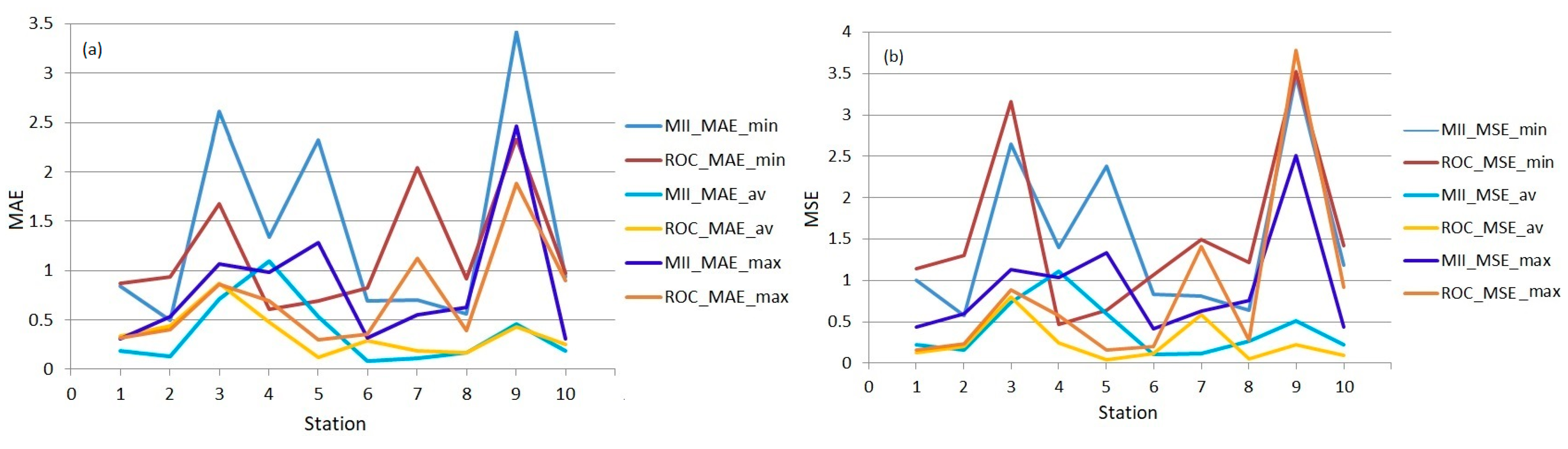
The worst results were obtained in both cases for the minimum ‘Regional series’, given that the series of minimum temperatures had a higher range than the other series. Comparisons between MAEs (MSEs) in all cases are provided in Figure 13. The following abbreviations were used in this figure: MII was the best model; min, max, and av denote the minimum, maximum, and average series; RCO is the abbreviation for ROCADA.
The highest MAEs and MSEs corresponded to Sulina (due to its particular position) and Constanta series (the station location was changed during the study period). Still, a good concordance between the model and the ROCADA series was noticed, confirming the model quality.
4. Conclusions
The article presents the regional evolution of the annual temperature series (minimum, average, maximum) for 1965–2005 in the Dobrogea region, Romania, using spatially distributed series. The methods were two original algorithms proposed by the author, versions of MPPM. The novelty of this approach is that instead of analyzing only the evolution of the individual series, a unique series for the entire region was built, selecting values from the data. Method II, which employs the clustering algorithm for selecting the series that participate in building the ‘Regional series’, provided better results than Method I in all situations.
To validate the results, the best ‘Regional series’ (in terms of MAE, and MSE) were compared with the series extracted from the ROCADA database (after processing to compute the maximum, minimum, and average series annual series). In all cases, the MAEs and MSEs of the fitted series were smaller than when they were measured with respect to the initial series.
An increasing trend of the minimum temperatures series was noticed, whereas the maximum (and average, with a smaller amplitude) regional series presented a high variability. More studies will be conducted on more recent data series to confirm these findings.
An interesting topic is related to the impact of the missing values (when they exist) on fitting the ‘Regional series’. Generally, the higher the number of missing values, the higher the error. The missing values may be replaced by values obtained by linear, spline, or wavelet interpolation of the data series recorded at the specified site or by the average of the data series. Another possibility is replacing the missing values with those recorded at neighboring stations. The study of the impact of the missing values will be extensively performed in the future.
Funding
The APC was funded by Transilvania University of Brasov, Romania by the funds for research.
Institutional Review Board Statement
Not applicable.
Informed Consent Statement
Not applicable.
Data Availability Statement
Data are available on request from the author.
Conflicts of Interest
The author declares no conflict of interest.
References
- Emadia, M.; Shahriarib, A.R.; Sadegh-Zadeha, F.; Seh-Bardana, B.J.; Dindarlou, A. Geostatistics-based spatial distribution of soil moisture and temperature regime classes in Mazandaran province, northern Iran. Arch. Acker Pfl. Boden. 2016, 62, 502–522. [Google Scholar] [CrossRef]
- Javari, M. Comparison of interpolation methods for modeling spatial variation of precipitation in Iran. Int. J. Environ. Sci. Ed. 2017, 12, 1037–1054. [Google Scholar]
- Chen, S.; Guo, J. Spatial interpolation techniques: Their applications in regionalizing climate-change series and associated accuracy evaluation in Northeast China. Geomat. Nat. Haz. Risk 2017, 8, 689–705. [Google Scholar] [CrossRef] [Green Version]
- Ozturk, D.; Kilik, F. Geostatistical Approach for Spatial Interpolation of Meteorological Data. An. Acad. Bras. Ciênc. 2016, 88, 2121–2136. [Google Scholar] [CrossRef] [Green Version]
- Wu, T.; Li, Y. Spatial interpolation of temperature in the United States using residual kriging. Appl. Geogr. 2013, 44, 112–120. [Google Scholar] [CrossRef]
- Goovaerts, P. Geostatistical approaches for incorporating elevation into the spatial interpolation of rainfall. J. Hydrol. 2000, 228, 113–129. [Google Scholar] [CrossRef]
- Thiessen, A.H. Precipitation for large areas. Mon. Weather Rev. 1911, 39, 1082–1084. [Google Scholar]
- Chiles, J.-P.; Delfiner, P. Geostatistics. Modeling Spatial Uncertainty, 2nd ed.; Wiley: Hoboken, NJ, USA, 2012. [Google Scholar]
- Ly, S.; Charles, C.; Degre, A. Different methods for spatial interpolation of rainfall data for operational hydrology and hydrological modeling at watershed scale: A review. Biotech. Agr. Soc. Environ. 2013, 17, 392–406. [Google Scholar]
- Szolgay, J.; Parajka, J.; Kohnova, S.; Hlavcova, K. Comparison of mapping approaches of design annual maximum daily precipitation. Atmos. Res. 2009, 92, 289–307. [Google Scholar] [CrossRef]
- Bărbulescu, A.; Băutu, A.; Băutu, E. Particle Swarm Optimization for the Inverse Distance Weighting Distance method. Appl. Sci. 2020, 10, 2054. [Google Scholar] [CrossRef] [Green Version]
- Șerban, C.; Bărbulescu, A.; Dumitriu, C.S. Maximum precipitation interpolation using an evolutionary optimized IDW algorithm. IOP Conf. Ser. Earth Env. Sci. 2022, 958, 012006. [Google Scholar] [CrossRef]
- Bărbulescu, A.; Șerban, C.; Indrecan, M.-L. Improving spatial interpolation quality. IDW versus a genetic algorithm. Water 2021, 13, 863. [Google Scholar] [CrossRef]
- Cressie, N.A.C. Statistics for Spatial Data; J. Wiley & Sons: Hoboken, NY, USA, 1993. [Google Scholar]
- Wadoux, A.M.J.-C.; Odeh, I.O.A.; McBratney, A.B. Overview of Pedometrics, in Reference Module in Earth Systems and Environmental Sciences, Elsevier, 2021. Available online: https://doi.org/10.1016/B978-0-12-822974-3.00001-X (accessed on 22 February 2023).
- Wong, A.H.; Kwon, T.J. Development and Evaluation of Geostatistical Methods for Estimating Weather Related Collisions: A Large-Scale Case Study. Transport. Res. Rec. 2021, 2675, 828–840. [Google Scholar] [CrossRef]
- Erdin, R.; Frei, C.; Künsch, H.R. Data Transformation and Uncertainty in Geostatistical Combination of Radar and Rain Gauges. J. Hydrometeorol. 2013, 13, 1332–1346. [Google Scholar] [CrossRef]
- Szentimrey, T.; Bihari, Z.; Szalai, S. Comparison of Geostatistical and Meteorological Interpolation Methods (What is What?). In Spatial Interpolation for Climate Data. The Use of GIS in Climatology and Meteorology; Dobesch, H., Dumolard, P., Dyras, I., Eds.; ISTE Ltd.: London, UK, 2007; pp. 45–56. [Google Scholar]
- Dumitrescu, A.; Birsan, M.-V. ROCADA: A gridded daily climatic dataset over Romania (1961–2013) for nine meteorological variables. Nat. Hazards 2015, 78, 1045–1063. [Google Scholar] [CrossRef]
- Mamara, A.; Anadranistakis, M.; Argiriou, A.A.; Szentimrey, T.; Kovacs, T.; Bezesc, A.; Bihari, Z. High resolution air temperature climatology for Greece for the period 1971–2000. Meteorol. Appl. 2017, 24, 191–205. [Google Scholar] [CrossRef] [Green Version]
- Gofa, F.; Mamara, A.; Anadranistakis, M.; Flocas, H. Developing Gridded Climate Data Sets of Precipitation for Greece Based on Homogenized Time Series. Climate 2019, 7, 68. [Google Scholar] [CrossRef] [Green Version]
- Szentimrey, T. Multiple Analysis of Series for Homogenization (MASH v1.02). Available online: http://www.dmcsee.org/uploads/file/330_1_mishmanual.pdf (accessed on 24 February 2023).
- Szentimrey, T.; Bihari, Z. Meteorological Interpolation based on Surface Homogenized Data Basis (MISH v3.02). Available online: http://www.dmcsee.org/uploads/file/331_2_mashmanual.pdf (accessed on 24 February 2023).
- Praveen, B.; Talukdar, S.; Shahfahad; Mahato, S.; Mondal, J.; Sharma, P.; Islam, A.R.M.T.; Rahman, A. Analyzing trend and forecasting of rainfall changes in India using non-parametrical and machine learning approaches. Sci. Rep. 2020, 10, 10342. [Google Scholar] [CrossRef]
- Patra, J.P.; Mishra, A.; Singh, R.; Raghuwanshi, N.S. Detecting rainfall trends in twentieth century (1871–2006) over Orissa State, India. Clim. Change 2012, 111, 801–817. [Google Scholar] [CrossRef]
- Bărbulescu, A.; Dumitriu, C.S.; Maftei, C. On the Probable Maximum Precipitation Method. Rom. J. Phys. 2022, 67, 801. [Google Scholar]
- Chatterjee, S.; Khan, A.; Akbari, H.; Wang, Y. Monotonic trends in spatio-temporal distribution and concentration of monsoon precipitation (1901–2002), West Bengal, India. Atmos. Res. 2016, 182, 54–75. [Google Scholar] [CrossRef]
- Zittis, G.; Bruggeman, A.; Lelieveld, J. Revisiting future extreme precipitation trends in the Mediterranean. Weather Clim. Extremes 2021, 34, 100380. [Google Scholar] [CrossRef] [PubMed]
- Huerta, G.; Sanso, B.; Stroud, J.R. A spatiotemporal model for Mexico city ozone levels. J. R. Stat. Soc. Ser. C 2004, 53, 231–248. Available online: https://www.jstor.org/stable/3592538 (accessed on 20 March 2022). [CrossRef] [Green Version]
- Lund, R.; Shao, Q.; Basawa, I. Parsimonious periodic time series modelling. Aust. NZ J. Stat. 2006, 48, 33–47. [Google Scholar] [CrossRef]
- Du, Z.; Wu, S.; Kwan, M.P.; Zhang, C.; Zhang, F.; Liu, R. A spatiotemporal regression-kriging model for space-time interpolation: A case study of chlorophyll-a prediction in the coastal areas of Zhejiang, China. Int. J. Geogr. Inf. Sci. 2018, 32, 1927–1947. [Google Scholar] [CrossRef]
- Im, H.K.; Rathouz, P.J.; Frederick, J.E. Space-time modelling of 20 years of daily air temperature in the Chicago metropolitan region. Environmetrics 2009, 20, 494–511. [Google Scholar] [CrossRef]
- Hijmans, R.J.; Cameron, S.E.; Parra, J.L.; Jones, P.G.; Jarvis, A. Very high resolution interpolated climate surfaces for global land areas. Int. J. Climatol. 2005, 25, 1965–1978. [Google Scholar] [CrossRef]
- Nalder, I.A.; Wein, R.W. Spatial interpolation of climatic normals: Test of a new method in the Canadian boreal forest. Agric. For. Meteor. 1998, 92, 211–225. [Google Scholar] [CrossRef]
- Wang, J.-F.; Reis, B.Y.; Hu, M.-G.; Christakos, G.; Yang, W.-Z.; Sun, Q.; Li, Z.-J.; Li, X.-Z.; Lai, S.-J.; Chen, H.-Y.; et al. Area Disease Estimation Based on Sentinel Hospital Records. PLoS ONE 2011, 6, e23428. [Google Scholar] [CrossRef] [PubMed] [Green Version]
- Xu, C.-D.; Wang, J.-F.; Hu, M.-G.; Li, Q.-X. Interpolation of missing temperature data at meteorological stations using P- BSHADE. J. Clim. 2013, 26, 7452–7463. [Google Scholar] [CrossRef]
- Xu, C.; Wang, J.; Li, Q. A New Method for Temperature Spatial Interpolation Based on Sparse Historical Stations. J. Clim. 2018, 31, 1757–1770. [Google Scholar] [CrossRef]
- Singh, G.; Soman, B. Spatial Interpolation using Inverse Distance Weighing (IDW) in R. Available online: https://rpubs.com/Dr_Gurpreet/interpolation_idw_R (accessed on 11 July 2022).
- Graler, B.; Pebesma, E.; Hevelink, G. Spatio-Temporal Interpolation Using Gstat. Available online: https://cran.r-project.org/web/packages/gstat/vignettes/spatio-termpoal-kriging.pdf (accessed on 11 July 2022).
- Spatiotemporal Interpolation Using Ensemble, ML. Available online: https://opengeohub.github.io/spatial-prediction-eml/spatiotemporal-interpolation-using-ensemble-ml.html (accessed on 11 July 2022).
- Bărbulescu, A. A new method for estimation the regional precipitation. Water Resour. Manag. 2016, 30, 33–42. [Google Scholar] [CrossRef]
- Bărbulescu, A.; Nazzal, Y.; Howari, F. Statistical analysis and estimation of the regional trend of aerosol size over the Arabian Gulf Region during 2002–2016. Sci. Rep. 2018, 8, 9571. [Google Scholar] [CrossRef] [PubMed] [Green Version]
- Bărbulescu, A. On the spatio-temporal characteristics of the aerosol optical depth in the Arabian Gulf zone. Atmosphere 2022, 13, 857. [Google Scholar] [CrossRef]
- Bărbulescu, A.; Postolache, F.; Dumitriu, C.Ș. Estimating the Precipitation Amount at Regional Scale Using a New Tool, Climate Analyzer. Hydrology 2021, 8, 125. [Google Scholar] [CrossRef]
- Kendall, M.G. Rank Correlation Methods, 4th ed.; Charles Griffin: London, UK, 1975. [Google Scholar]
- Sen, P.K. Estimates of the regression coefficient based on Kendall’s tau. J. Am. Stat. Assoc. 1968, 63, 1379–1389. [Google Scholar] [CrossRef]
- Kruskal-Wallis Test. Available online: https://www.statsdirect.com/help/default.htm#nonparametric_methods/kruskal_wallis.htm (accessed on 12 June 2022).
- Yudha Wijaya, C. Breaking down the Agglomerative Clustering Process. Available online: https://towardsdatascience.com/breaking-down-the-agglomerative-clustering-process-1c367f74c7c2 (accessed on 12 June 2022).
- Kaufman, L.; Rousseeuw, P.J. Finding Groups in Data: An Introduction to Cluster Analysis; Wiley: New York, NY, USA, 1990. [Google Scholar]
- Difference between K Means and Hierarchical Clustering. Available online: https://www.geeksforgeeks.org/difference-between-k-means-and-hierarchical-clustering/ (accessed on 20 March 2022).
- Scott, A.J.; Symons, M.J. Clustering Methods Based on Likelihood Ratio Criteria. Biometrics 1971, 27, 387–397. [Google Scholar] [CrossRef] [Green Version]
- Marriot, F.H.C. Practical Problems in a Method of Cluster Analysis. Biometrics 1971, 27, 501–514. [Google Scholar] [CrossRef]
- Hubert, L.J.; Arabie, P. Comparing Partitions. J. Classif. 1985, 2, 193–218. [Google Scholar] [CrossRef]
- Friedman, H.P.; Rubin, J. On Some Invariant Criteria for Grouping Data. J. Am. Stat. Assoc. 1967, 62, 1159–1178. [Google Scholar] [CrossRef]
- Rousseeuw, P. Silhouettes: A Graphical Aid to the Interpretation and Validation of Cluster Analysis. J. Comput. Appl. Math. 1987, 20, 53–65. [Google Scholar] [CrossRef] [Green Version]
- Tibshirani, R.; Walther, G.; Hastie, T. Estimating the number of clusters in a data set via the gap statistic. J. R. Stat. Soc. B 2001, 63, 411–423. [Google Scholar] [CrossRef]
- Charrad, M.; Ghazzali, N.; Boiteau, V.; Niknafs, A. NbClust: An R Package for Determining the Relevant Number of Clusters in a Data Set. J. Stat. Softw. 2014, 61, 1–36. [Google Scholar] [CrossRef] [Green Version]
- Lafitte, P. Traité D’informatique Geologique; Masson & Cie: Paris, France, 1972. [Google Scholar]
- Shepard, D. A two-dimensional interpolation function for irregularly spaced data. In Proceedings of the 1968 ACM National Conference, Las Vegas, NV, USA, 27–29 August 1968; pp. 517–524. [Google Scholar]
- Maftei, C.; Bărbulescu, A. Statistical analysis of climate evolution in Dobrudja region. Lect. Notes Eng. Comput. Sci. 2008, 2, 1082–1087. [Google Scholar]
- Mocanu-Vargancsik, C.A.; Bărbulescu, A. Study of the Temperature’s Evolution Trend on the Black Sea Shore at Constanta. J. Phys. Conf. Ser. 2019, 1297, 012010. [Google Scholar] [CrossRef]
- Bărbulescu, A. Modeling temperature evolution. Case study. Rom. Rep. Phys. 2016, 68, 798. [Google Scholar]
- Bărbulescu, A. Models for temperature evolution in Constanta area (Romania). Rom. J. Phys 2016, 61, 676–686. [Google Scholar]
- Bărbulescu, A.; Deguenon, J. About the variations of precipitation and temperature evolution in the Romanian Black Sea Littoral. Rom. Rep. Phys. 2015, 67, 625–637. [Google Scholar]
- Bărbulescu, A.; Băutu, E. Mathematical models of climate evolution in Dobrudja. Theor. Appl. Climatol. 2010, 100, 29–44. [Google Scholar] [CrossRef]
- Dumitriu, C.S.; Bărbulescu, A.; Maftei, C. IrrigTool—A New Tool for Determining the Irrigation Rate Based on Evapotranspiration Estimated by the Thornthwaite Equation. Water 2022, 67, 2399. [Google Scholar] [CrossRef]
- Maftei, C.; Bărbulescu, A.; Rugină, S.; Nastac, C.D.; Dumitru, I.M. Analysis of the arbovirosis potential occurrence in Dobrogea, Romania. Water 2021, 13, 374. [Google Scholar] [CrossRef]
- Bărbulescu, A.; Postolache, F. New approaches for modeling the regional pollution in Europe. Sci. Total Environ. 2021, 753, 141993. [Google Scholar] [CrossRef] [PubMed]
Figure 1.
The study flowchart. Sim_no means the number of simulations.

Figure 3.
Minimum, maximum, and mean annual series.

Figure 4.
The case of two intervals/clusters for the series of minimum temperatures: (a) ‘Regional series’; (b) MAE and MSE—Method I; (c) MAE and MSE—Method II; (d) comparisons of MAEs; (e) comparisons of MSEs; (f) min, max, and amplitude of the minimum temperature series.
Figure 4.
The case of two intervals/clusters for the series of minimum temperatures: (a) ‘Regional series’; (b) MAE and MSE—Method I; (c) MAE and MSE—Method II; (d) comparisons of MAEs; (e) comparisons of MSEs; (f) min, max, and amplitude of the minimum temperature series.

Figure 5.
The case of three intervals/clusters for the series of minimum temperatures: (a) ‘Regional series’; (b) MAE and MSE—Method I; (c) MAE and MSE—Method II; (d) comparisons of MAEs; (e) comparisons of MSEs; (f) min, max, and amplitude of the minimum temperature series.
Figure 5.
The case of three intervals/clusters for the series of minimum temperatures: (a) ‘Regional series’; (b) MAE and MSE—Method I; (c) MAE and MSE—Method II; (d) comparisons of MAEs; (e) comparisons of MSEs; (f) min, max, and amplitude of the minimum temperature series.

Figure 6.
Comparison between the results on the minimum temperatures for two and three intervals/clusters: (a) Method I—MAE; (b) Method I—MSE; (c) Method I—‘Regional series’; (d) Method II—MAE; (e) Method II—MSE; (f) Method II—‘Regional series’.
Figure 6.
Comparison between the results on the minimum temperatures for two and three intervals/clusters: (a) Method I—MAE; (b) Method I—MSE; (c) Method I—‘Regional series’; (d) Method II—MAE; (e) Method II—MSE; (f) Method II—‘Regional series’.

Figure 7.
The case of two intervals/clusters for the series of average temperatures: (a) the regional series, (b) MAE and MSE—Method I; (c) MAE and MSE—Method II; (d) comparisons of MAEs; (e) comparisons of MSEs; (f) min, max, and amplitude of the average temperatures series.
Figure 7.
The case of two intervals/clusters for the series of average temperatures: (a) the regional series, (b) MAE and MSE—Method I; (c) MAE and MSE—Method II; (d) comparisons of MAEs; (e) comparisons of MSEs; (f) min, max, and amplitude of the average temperatures series.

Figure 8.
The case of three intervals/clusters for the series of average temperatures: (a) the regional series, (b) MAE and MSE—Method I; (c) MAE and MSE—Method II; (d) comparisons of MAEs; (e) comparisons of MSEs; (f) min, max, and amplitude of the average temperatures series.
Figure 8.
The case of three intervals/clusters for the series of average temperatures: (a) the regional series, (b) MAE and MSE—Method I; (c) MAE and MSE—Method II; (d) comparisons of MAEs; (e) comparisons of MSEs; (f) min, max, and amplitude of the average temperatures series.
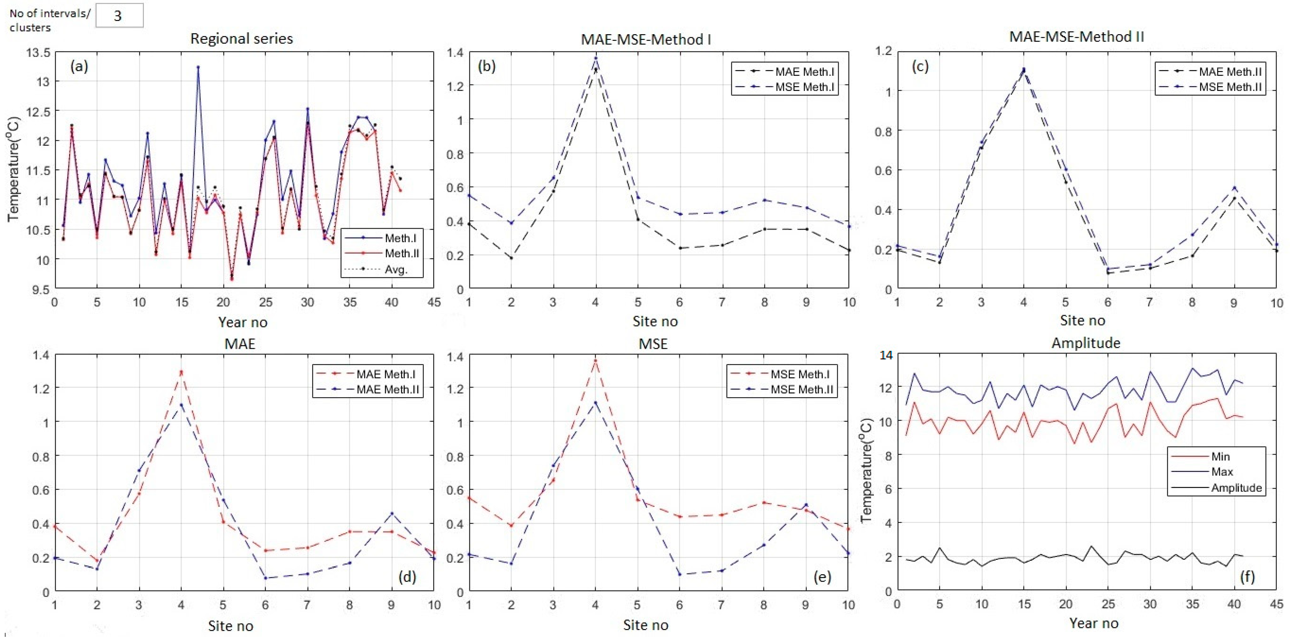
Figure 9.
Comparison between the ‘Regional series’ of the average temperatures for two and three intervals/clusters: (a) Method I—MAE; (b) Method I—MSE; (c) Method I—‘Regional series’; (d) Method II—MAE; (e) Method II—MSE; (f) Method II—‘Regional series’.
Figure 9.
Comparison between the ‘Regional series’ of the average temperatures for two and three intervals/clusters: (a) Method I—MAE; (b) Method I—MSE; (c) Method I—‘Regional series’; (d) Method II—MAE; (e) Method II—MSE; (f) Method II—‘Regional series’.
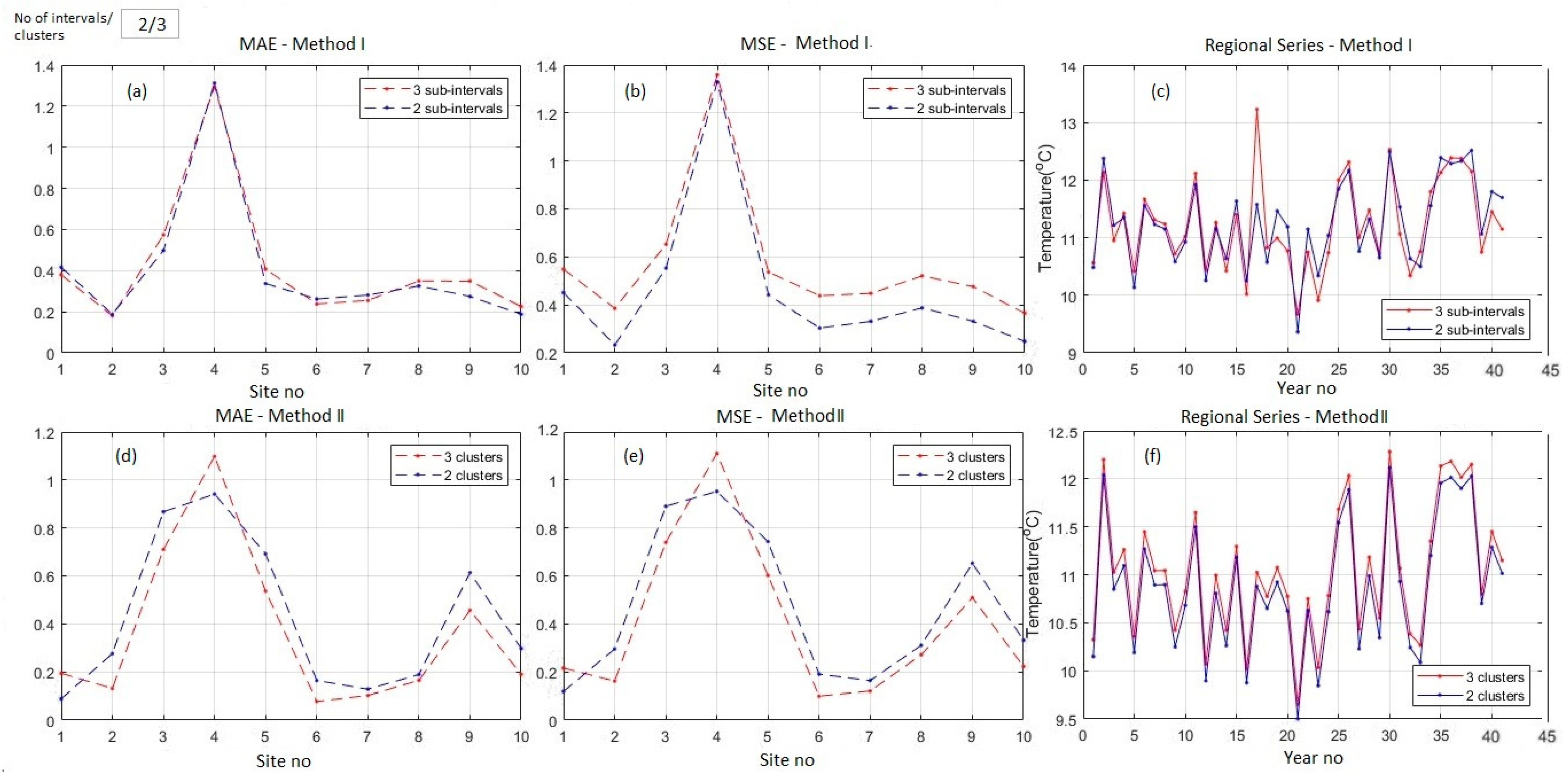
Figure 10.
The case of two intervals/clusters for the series of maximum temperatures: (a) the regional series; (b) MAE and MSE—Method I; (c) MAE and MSE—Method II; (d) comparisons of MAEs; (e) comparisons of MSEs; (f) min, max, and amplitude of the average temperatures series.
Figure 10.
The case of two intervals/clusters for the series of maximum temperatures: (a) the regional series; (b) MAE and MSE—Method I; (c) MAE and MSE—Method II; (d) comparisons of MAEs; (e) comparisons of MSEs; (f) min, max, and amplitude of the average temperatures series.

Figure 11.
The case of three intervals/clusters for the series of maximum temperatures: (a) the regional series; (b) MAE and MSE—Method I; (c) MAE and MSE—Method II; (d) comparisons of MAEs; (e) comparisons of MSEs; (f) min, max, and amplitude of the average temperatures series.
Figure 11.
The case of three intervals/clusters for the series of maximum temperatures: (a) the regional series; (b) MAE and MSE—Method I; (c) MAE and MSE—Method II; (d) comparisons of MAEs; (e) comparisons of MSEs; (f) min, max, and amplitude of the average temperatures series.

Figure 12.
The case of two and three intervals/clusters for the series of maximum temperatures: (a) the regional series; (b) MAE and MSE—Method I; (c) MAE and MSE—I; (d) comparisons of MAEs; (e) comparisons of MSEs; (f) min, max, and amplitude of the average temperatures series.
Figure 12.
The case of two and three intervals/clusters for the series of maximum temperatures: (a) the regional series; (b) MAE and MSE—Method I; (c) MAE and MSE—I; (d) comparisons of MAEs; (e) comparisons of MSEs; (f) min, max, and amplitude of the average temperatures series.
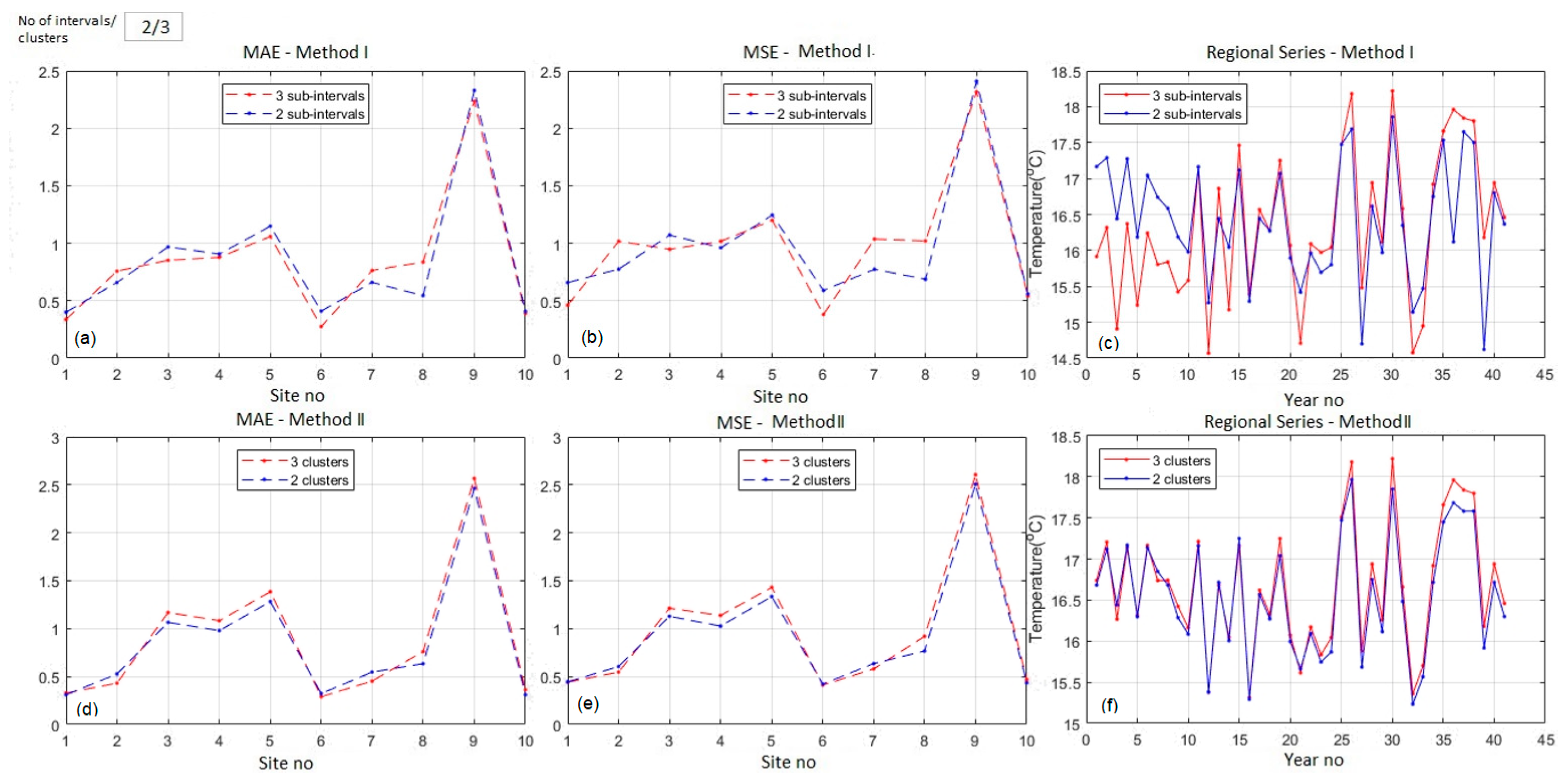
Figure 13.
Comparisons between (a) MAEs and (b) MSEs from the models.

Table 1.
Results of the Mann–Kendall trend test.
| Series | Minimum Series | Average Series | Maximum Series | ||||||
|---|---|---|---|---|---|---|---|---|---|
| Station | Signific. | Q | B | Signific. | Q | B | Signific. | Q | B |
| Adamclisi | + | 0.015 | 6.37 | 0.015 | 10.55 | * | 0.023 | 15.93 | |
| Cernavoda | *** | 0.084 | 4.06 | 0.013 | 10.84 | −0.013 | 17.21 | ||
| Constanta | * | 0.024 | 8.06 | + | 0.020 | 11.40 | * | 0.025 | 15.05 |
| Corugea | *** | 0.078 | 3.04 | + | 0.018 | 9.60 | −0.014 | 15.70 | |
| Harsova | *** | 0.076 | 3.84 | 0.013 | 10.70 | −0.015 | 17.36 | ||
| Jurilovca | *** | 0.097 | 3.93 | 0.014 | 10.67 | ** | −0.031 | 16.62 | |
| Mangalia | * | 0.020 | 7.68 | + | 0.019 | 11.27 | 0.016 | 14.98 | |
| Medgidia | * | 0.024 | 6.03 | 0.013 | 10.70 | * | 0.026 | 15.90 | |
| Sulina | + | 0.018 | 9.00 | 0.017 | 11.25 | * | 0.025 | 13.73 | |
| Tulcea | −0.003 | 6.76 | 0.017 | 10.85 | 0.013 | 16.19 | |||
Note: *** significance level 0.001, ** significance level 0.01, * significance level 0.05, blank cell means a significance level of 0.1.
Table 2.
Comparative results of Methods I and II for minimum temperatures series (°C).
| Method I | Method II | ||||||||
|---|---|---|---|---|---|---|---|---|---|
| MAE | MSE | MAE | MSE | ||||||
| n | 2 | 3 | 2 | 3 | 2 | 3 | 2 | 3 | |
| Site No. | |||||||||
| 1 | 0.77 | 1.32 | 0.92 | 1.67 | 0.84 | 1.43 | 1.00 | 1.73 | |
| 2 | 1.14 | 0.41 | 1.80 | 0.66 | 0.50 | 0.29 | 0.58 | 0.32 | |
| 3 | 1.98 | 3.01 | 2.17 | 3.20 | 2.61 | 3.19 | 2.65 | 3.33 | |
| 4 | 1.96 | 0.93 | 2.44 | 1.17 | 1.34 | 0.76 | 1.40 | 0.78 | |
| 5 | 1.70 | 2.75 | 1.95 | 2.95 | 2.32 | 2.90 | 2.38 | 3.06 | |
| 6 | 0.74 | 1.20 | 0.89 | 1.52 | 0.69 | 1.28 | 0.83 | 1.56 | |
| 7 | 1.34 | 0.31 | 1.98 | 0.69 | 0.70 | 0.14 | 0.81 | 0.19 | |
| 8 | 1.22 | 0.57 | 1.69 | 0.76 | 0.56 | 0.57 | 0.64 | 0.65 | |
| 9 | 2.80 | 3.82 | 2.96 | 4.01 | 3.42 | 4.00 | 3.47 | 4.13 | |
| 10 | 0.75 | 1.43 | 1.01 | 1.82 | 0.94 | 1.53 | 1.18 | 1.91 | |
| Average | 1.44 | 1.58 | 1.78 | 1.85 | 1.39 | 1.61 | 1.50 | 1.77 | |
Table 3.
Comparative results of the output for average temperatures series (°C) for n = 2 and n = 3.
Table 3.
Comparative results of the output for average temperatures series (°C) for n = 2 and n = 3.
| Method I | Method II | ||||||||
|---|---|---|---|---|---|---|---|---|---|
| MAE | MSE | MAE | MSE | ||||||
| n | 2 | 3 | 2 | 3 | 2 | 3 | 2 | 3 | |
| Site No. | |||||||||
| 1 | 0.41 | 0.38 | 0.45 | 0.55 | 0.09 | 0.19 | 0.12 | 0.22 | |
| 2 | 0.19 | 0.18 | 0.23 | 0.38 | 0.27 | 0.13 | 0.30 | 0.16 | |
| 3 | 0.50 | 0.57 | 0.55 | 0.65 | 0.87 | 0.71 | 0.89 | 0.74 | |
| 4 | 1.31 | 1.29 | 1.33 | 1.36 | 0.94 | 1.10 | 0.95 | 1.11 | |
| 5 | 0.34 | 0.41 | 0.44 | 0.54 | 0.69 | 0.53 | 0.74 | 0.60 | |
| 6 | 0.26 | 0.24 | 0.30 | 0.44 | 0.16 | 0.08 | 0.19 | 0.10 | |
| 7 | 0.28 | 0.25 | 0.33 | 0.45 | 0.13 | 0.11 | 0.16 | 0.12 | |
| 8 | 0.32 | 0.35 | 0.39 | 0.52 | 0.19 | 0.17 | 0.31 | 0.27 | |
| 9 | 0.27 | 0.35 | 0.33 | 0.47 | 0.61 | 0.46 | 0.65 | 0.51 | |
| 10 | 0.19 | 0.23 | 0.25 | 0.36 | 0.30 | 0.19 | 0.33 | 0.22 | |
| Average | 0.41 | 0.43 | 0.46 | 0.57 | 0.43 | 0.37 | 0.46 | 0.41 | |
Table 4.
Comparative results of Methods I and II for the maximum temperatures series for two and three intervals/clusters (°C).
Table 4.
Comparative results of Methods I and II for the maximum temperatures series for two and three intervals/clusters (°C).
| Method I | Method II | ||||||||
|---|---|---|---|---|---|---|---|---|---|
| MAE | MSE | MAE | MSE | ||||||
| n | 2 | 3 | 2 | 3 | 2 | 3 | 2 | 3 | |
| Site No. | |||||||||
| 1 | 0.40 | 0.37 | 0.66 | 0.46 | 0.31 | 0.33 | 0.44 | 0.44 | |
| 2 | 0.66 | 0.76 | 0.77 | 1.02 | 0.53 | 0.43 | 0.60 | 0.54 | |
| 3 | 0.97 | 0.85 | 1.07 | 0.95 | 1.07 | 1.17 | 1.13 | 1.21 | |
| 4 | 0.91 | 0.88 | 0.96 | 1.02 | 0.98 | 1.09 | 1.03 | 1.14 | |
| 5 | 1.15 | 1.06 | 1.25 | 1.19 | 1.28 | 1.38 | 1.33 | 1.43 | |
| 6 | 0.41 | 0.27 | 0.59 | 0.38 | 0.32 | 0.29 | 0.42 | 0.41 | |
| 7 | 0.66 | 0.76 | 0.77 | 1.04 | 0.55 | 0.46 | 0.63 | 0.58 | |
| 8 | 0.55 | 0.84 | 0.69 | 1.02 | 0.63 | 0.76 | 0.76 | 0.92 | |
| 9 | 2.33 | 2.23 | 2.41 | 2.32 | 2.46 | 2.56 | 2.51 | 2.61 | |
| 10 | 0.41 | 0.39 | 0.56 | 0.54 | 0.31 | 0.36 | 0.44 | 0.47 | |
| Average | 0.84 | 0.84 | 0.97 | 0.99 | 0.84 | 0.88 | 0.93 | 0.99 | |
Table 5.
Comparison of the best results from Methods I and II and IDW (°C).
| Min | Average | Max | ||||||||||
|---|---|---|---|---|---|---|---|---|---|---|---|---|
| MAE | MSE | MAE | MSE | MAE | MSE | |||||||
| Site No. | MII | ROC | MII | ROC | MII | ROC | MII | ROC | MII | ROC | MII (2) | ROC |
| 1 | 0.84 | 0.87 | 1.00 | 1.14 | 0.19 | 0.34 | 0.22 | 0.13 | 0.31 | 0.32 | 0.44 | 0.16 |
| 2 | 0.50 | 0.94 | 0.58 | 1.30 | 0.13 | 0.44 | 0.16 | 0.20 | 0.53 | 0.40 | 0.60 | 0.23 |
| 3 | 2.61 | 1.68 | 2.65 | 3.16 | 0.71 | 0.87 | 0.74 | 0.80 | 1.07 | 0.86 | 1.13 | 0.88 |
| 4 | 1.34 | 0.61 | 1.40 | 0.47 | 1.10 | 0.48 | 1.11 | 0.24 | 0.98 | 0.69 | 1.03 | 0.58 |
| 5 | 2.32 | 0.69 | 2.38 | 0.64 | 0.53 | 0.12 | 0.60 | 0.04 | 1.28 | 0.30 | 1.33 | 0.16 |
| 6 | 0.69 | 0.82 | 0.83 | 1.07 | 0.08 | 0.29 | 0.10 | 0.12 | 0.32 | 0.36 | 0.42 | 0.20 |
| 7 | 0.70 | 2.04 | 0.81 | 1.49 | 0.11 | 0.19 | 0.12 | 0.59 | 0.55 | 1.12 | 0.63 | 1.41 |
| 8 | 0.56 | 0.92 | 0.64 | 1.22 | 0.17 | 0.17 | 0.27 | 0.05 | 0.63 | 0.39 | 0.76 | 0.28 |
| 9 | 3.42 | 2.34 | 3.47 | 3.52 | 0.46 | 0.43 | 0.51 | 0.22 | 2.46 | 1.88 | 2.51 | 3.78 |
| 10 | 0.94 | 0.97 | 1.18 | 1.42 | 0.19 | 0.25 | 0.22 | 0.09 | 0.31 | 0.90 | 0.44 | 0.92 |
| Average | 1.39 | 1.18 | 1.49 | 1.54 | 0.37 | 0.36 | 0.41 | 0.25 | 0.84 | 0.72 | 0.93 | 0.85 |
Disclaimer/Publisher’s Note: The statements, opinions and data contained in all publications are solely those of the individual author(s) and contributor(s) and not of MDPI and/or the editor(s). MDPI and/or the editor(s) disclaim responsibility for any injury to people or property resulting from any ideas, methods, instructions or products referred to in the content. |
© 2023 by the author. Licensee MDPI, Basel, Switzerland. This article is an open access article distributed under the terms and conditions of the Creative Commons Attribution (CC BY) license (https://creativecommons.org/licenses/by/4.0/).
Share and Cite
MDPI and ACS Style
Bărbulescu, A. On the Regional Temperature Series Evolution in the South-Eastern Part of Romania. Appl. Sci. 2023, 13, 3904. https://doi.org/10.3390/app13063904
AMA Style
Bărbulescu A. On the Regional Temperature Series Evolution in the South-Eastern Part of Romania. Applied Sciences. 2023; 13(6):3904. https://doi.org/10.3390/app13063904
Chicago/Turabian StyleBărbulescu, Alina. 2023. "On the Regional Temperature Series Evolution in the South-Eastern Part of Romania" Applied Sciences 13, no. 6: 3904. https://doi.org/10.3390/app13063904
Note that from the first issue of 2016, this journal uses article numbers instead of page numbers. See further details here.