Evaluation of System Identification Methods for Free Vibration Flutter Derivatives of Long-Span Bridges

Abstract

The significance of long-span bridges being susceptible to wind-induced vibrations and the need for evaluating their aerodynamic performance is the focus of this study. The main emphasis is on experimental methods for assessing the bridges’ aerodynamic stability, using sectional model tests with the free vibration technique. The dynamic properties of the model are determined from the measured response, using various system identification methods, including the modified Ibrahim time domain (MITD) and iterative least squares (ILS) for two-degree-of-freedom systems and the logarithmic decrement method (LDM) and the Hilbert transform method (HTM) for single-degree-of-freedom (SDOF) systems. A new dynamic testing setup was designed to facilitate single-degree-of-freedom (heave and pitch) and coupled two-degree-of-freedom (2DOF) motion in a wind tunnel section model. The vertical and torsional stiffnesses of the model were adjusted with elastic springs. A Great Belt Bridge section model was selected for testing due to its streamlined aerodynamic shape. The direct and crossflow derivatives were extracted from the measured response using the system identification methods mentioned. Additionally, analytical studies and numerical computational fluid dynamics simulations were conducted to validate the experimental results. The study found that HTM is most effective in SDOF due to its ability to extract both damping and frequency from the nonlinear response, whereas the MITD method is faster in converging system parameters in 2DOF system tests. The experimental and numerical results are comparable to the flat plate, which confirms the streamlined behavior of the Great Belt section from an aerodynamic perspective.

1. Introduction

Long-span bridges play a crucial role in civil engineering and are considered major engineering feats. Since the construction of the Brooklyn Bridge in 1883, the design of modern suspension bridges has greatly advanced. The span length of suspension bridges rapidly increased from 486 m for the Brooklyn Bridge to 1067 m for the George Washington Bridge in 1931 and up to 1991 m for the Akashi Kaikyo Bridge in 1998 [1,2]. The design of these bridges is constantly advancing along with the materials of construction [3], allowing engineers to construct longer, slender, and more flexible structures [4]. However, the flexible nature of these structures requires precise assessments of their aerodynamic properties for stability and safety [5]. For example, pipeline suspension bridges, used for water, oil, or gas transportation, can be highly sensitive to wind due to their narrowness, lightness, and flexibility [6]. In addition, non-engineering defects can also contribute to the failure of reinforced structures [7].

Wind-induced vibrations on long-span bridges are a complex phenomenon that can cause significant structural damage if not properly addressed. During construction, these bridges are especially vulnerable as the main cables are hung from the bridge towers and are not supported by a stiffening girder, leading to low rigidity and sensitivity to wind excitations [8,9]. This has been demonstrated by several bridges in China that experienced large-amplitude, wind-induced vibrations during construction, posing a risk to both structures and workers. Substructure failures, such as in piles, also cause numerous bridge failures [10], and it is crucial to understand the importance of predicting appropriate pile displacement responses in linear elastic soil systems [11,12].

Historically, wind loads have been treated as static, but they can cause structural resonance [13]. Vibrations caused by the wind’s interaction with the bridge’s structure can excite resonant frequencies, leading to excessive motion. This can result in fatigue damage, cracking, and even collapse if left unmitigated. Engineers employ various techniques, such as aerodynamic shaping, dampers, and tuned mass dampers, to reduce wind-induced vibrations on long-span bridges. Aerodynamic measures are commonly used to enhance the wind-induced vibration performance of bridges. Some nondestructive testing methodologies, such as magnetic flux leakage, can also be employed to detect early damage in long-span bridges [14]. Wind tunnel tests are frequently conducted to study the performance of these measures. Sectional model tests with large-scale ratios are often used to measure aerodynamic coefficients, analyze vortex-induced vibrations (VIVs), and investigate two-degree-of-freedom flutter [15]. The effects of handrails and wind-fairing guide vanes on bridge aerodynamics can also be studied through sectional model tests. Full-bridge aeroelastic model tests can accurately simulate the multi-order modal responses and wind-induced vibrations of the bridge in actual atmospheric boundary conditions [16]. Tests have shown that suitable wind fairing can improve flutter stability and reduce VIV response [17,18].

The collapse of the Tacoma Narrows Bridge in 1940 is a famous example of wind-induced vibrations on a long-span bridge [19]. These vibrations can manifest as flutter, galloping, VIVs, or random buffeting. Flutter and VIVs are the primary forms of wind-induced instability vibrations that pose the greatest threat to the safety of long-span bridges [20]. The bridge’s collapse was due to aeroelastic flutter, which was caused by the wind’s interaction with the bridge’s structure. Flutter can lead to structural collapse after amplitude divergence, while VIVs cause bending or torsional single-mode vibrations that affect driver and pedestrian comfort. During the construction of the Old Tacoma Narrows Bridge, VIVs were present and transformed into flutter just prior to the bridge’s collapse.

Ref. [21] notes that, in the early 2000s, engineers found that the Sydney Harbor Bridge was experiencing excessive wind-induced vibrations and installed tuned mass dampers to address the issue. These devices reduce vibrations by absorbing energy [21]. The Millau Viaduct in France, with a main span of 2460 m, underwent extensive wind tunnel testing and numerical simulations to evaluate its aerodynamic performance. The Tower Bridge in London recently underwent a renovation, which included the installation of wind sensors and a weather station to monitor wind conditions and optimize the bridge’s operation and maintenance. The Akashi Kaikyo Bridge in Japan also underwent full aeroelastic model testing using a big boundary layer wind tunnel, which helped engineers develop design considerations for wind effects on the bridge [22]. These examples indicate a strong need for comprehensive aerodynamic model testing especially when additive manufacturing is prevailing in the bridge industry [23].

The Great Belt Bridge, which connects the Danish islands of Funen and Zealand, is a three-span suspension bridge and one of the longest bridges in the world. Suspension bridges are the most efficient form of long-span bridges because of their low stiffness, but they also become more flexible with increasing span and have prominent dynamic problems [24]. Wind tunnel testing is the best option for checking the aerodynamics and aeroelasticity of long-span bridges and can be classified into three types: sectional model testing, taut strip model testing, and full aeroelastic model testing. In this research, a section of the Great Belt Bridge has been selected as a reference to perform wind tunnel testing due to its streamlined aerodynamic shape. A novel testing setup is designed, which facilitates a single-degree-of-freedom (heave and pitch) and coupled two-degree-of-freedom motion to a wind tunnel section model. The direct and cross-flutter derivatives are obtained from the measured data using several system identification methods, including the Hilbert transform method, the logarithmic decrement method, the iterative least squares method, and the modified Ibrahim time domain method. Furthermore, an analytical study along with numerical computational fluid dynamic simulations are also performed to validate the experimental results.

2. Aerodynamic Phenomena

Aeroelastic or aerodynamic phenomena occur due to interactions between wind and structure. When a structure vibrates in response to an oncoming flow, it changes the flow pattern, which, in turn, affects the structural vibrations. The aerodynamic behavior of long-span bridges can be classified into two groups based on the magnitude of vibrations under wind action: limited amplitude and divergent amplitude.

2.1. Limited Amplitude Phenomena

These phenomena occur at a restricted range of wind speeds, and this group encompasses buffeting, vortex-induced vibrations (VIV), rain–wind-induced vibrations, and wake-induced vibrations, which cause discomfort in serviceability, increase internal stresses, and may lead to fatigue in the bridge structure.

2.1.1. Vortex-Induced Vibrations (VIVs)

Vortex-induced vibrations (VIV) are motions experienced by structures due to their interaction with the flow, caused by vortex shedding in the wake. This leads to fluctuating pressures on the structure’s surface, causing oscillations perpendicular to the flow direction. The frequency of these vortices depends on flow velocity, the shape of the body, and fluid viscosity. Lock-in, a phenomenon in long-span bridges, occurs when the vortex shedding frequency aligns with one of the bridge’s natural frequencies, leading to strong, sustained oscillations for a specific wind-speed range. Past examples of bridges experiencing VIVs include the Great Belt Bridge, the Trans-Tokyo Bay Highway, the Niteroi Bridge, the Volgograd Bridge, and the Arches of Alconetar bridge during the construction [25,26,27,28].

2.1.2. Buffeting

The buffeting response of a long-span bridge is a random vibration caused by the fluctuating pressure resulting from the natural turbulence in the oncoming wind. If it occurs due to the wake of the structure on the upstream side, it is referred to as wake buffeting. The buffeting response of the bridge depends on its natural frequencies, the shape of the deck, and the turbulence intensity. The structural response from buffeting increases monotonically with an increase in wind speed.

2.2. Divergent Amplitude Phenomena

The divergent amplitude of a structure is caused by self-excited forces from wind–structure interactions. If the input energy from the wind is less than the energy dissipated by the structure, the amplitudes will decrease. However, if damping is insufficient, amplitudes will increase and could result in failure. The wind speed that triggers the diverging motion is called the critical wind speed.

2.2.1. Classical Flutter

Classical flutter is a two-degree-of-freedom aerodynamic instability where vertical and torsional modes couple in flow-driven unstable oscillations with energy transfer between the modes. It is also known as 2DOF flutter or coupled flutter. Energy transfer only occurs when the contributing degree of freedom has the same frequency, also known as the flutter frequency.

2.2.2. Galloping

Galloping is a single-degree-of-freedom (SDOF) aerodynamic instability where the aerodynamic damping in the crosswind direction becomes negative, causing large transverse amplitudes. It is also referred to as “crosswind galloping”, “translational galloping”, or “bending flutter”. Slender structures with large depth-to-width ratios are more prone to hard galloping, while those with smaller ratios have a higher likelihood of soft galloping.

2.2.3. Torsional Flutter

Torsional flutter is a single-degree-of-freedom (SDOF) aerodynamic instability in rotational motion, also referred to as “rotational galloping”. It occurs when the effective damping (mechanical and aerodynamic) of the structure in torsional motion becomes zero. Long-span bridges with a broad deck cross-section are more susceptible to torsional flutter, while bridges with streamlined deck sections tend to exhibit classical flutter.

2.2.4. Torsional Divergence

Torsional divergence, also known as static-type instability, is linked to the torsional stiffness of a structure. It occurs when the combined stiffness of the structure and its aerodynamics reaches zero, usually at high wind speeds, and is considered the ultimate limit state.

3. Methods of Aerodynamic Analysis

The aerodynamic analysis of a bridge can be performed by using experimental methods (wind tunnel test), analytical methods (Theodorsen theory), and by using numerical methods (computational fluid dynamics).

3.1. Wind Tunnel Testing

Wind tunnel tests are very important in bridge response investigations and designs. The scaling of structural and flow properties using nondimensional parameters such as the Froude number, the Reynolds number, and the Strouhal number is applied in model and experimental designs. Notable long-span bridges such as Stonecutters Bridge, the Great Belt Bridge, and Akashi Kaikyo Bridge underwent extensive wind tunnel tests during design [29]. There are three types of models used for these tests depending on the type of tests, costs, and time constraints. Section model testing is used in current research, and it involves testing a scaled cross-section of the bridge’s main section. Section model tests are more conservative in predicting bridge instabilities and can be used in the early design stage to identify the best aerodynamic cross-sectional shape. Taut-strip models are simpler than full aeroelastic models. They consist of a bridge deck connected to two parallel taut wires in the wind tunnel section. This approach is less expensive and can target several modes and the 3D structure of turbulence. Full 3D models are scaled replicas of actual bridges, including all structural details. Full aeroelastic models are typically used as a final check for a bridge’s aerodynamic characteristics due to their high cost.

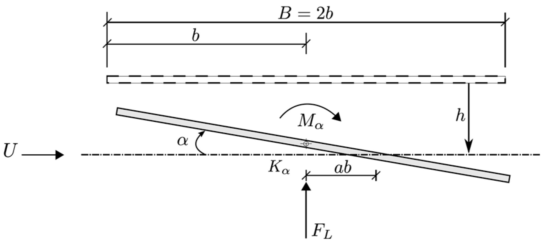
3.2. Theodorsen Theory for Flat Plate

The Theodorsen [30] approach for flutter analysis uses potential flow theory and is based on the idea that, for a thin airfoil in an incompressible flow, lift (F_L) and moment (F_M) are linear functions of displacement (h) and rotation (α), and their first derivatives are shown in Figure 1. This approach is only valid for streamlined cross-sections and does not depend on the shape of the body. Theodorsen considered a flat plate exposed to an oncoming flow undergoing small harmonic oscillations in the vertical (h) and rotation (α) values at a distance, “ab”, from its center.

The Theodorsen functions for the symmetrical deck section (a = 0) can also be represented in terms of aerodynamic derivatives, which are as follows [30]:

$$\begin{array}{ll}{H}_1^{*}=-\frac{2\pi }{K}F& ,A_1^{*}=\frac{2\pi }{K}F\\ H_2^{*}=-\frac{\pi }{2K}\left[1+\frac{4G}{K}+F\right]& ,A_2^{*}=-\frac{\pi }{2K^2}\left[\frac{K}{4}-G-\frac{KF}{4}\right]\\ H_3^{*}=-\frac{\pi }{K^2}\left[2F-\frac{GK}{2}\right]& ,A_3^{*}=\frac{\pi }{{2K}^2}\left[\frac{K^2}{32}+F-\frac{KG}{4}\right]\\ H_4^{*}=\frac{\pi }{2}\left[1+\frac{4G}{K}\right]& ,A_4^{*}=-\frac{\pi }{2K}G\end{array}$$

3.3. Numerical Methods

Numerical methods, including computational fluid dynamics (CFD) and computational wind engineering (CWE), are growing in popularity due to recent advancements in computer modeling and analysis techniques. While wind tunnel tests are still considered reliable, they have restrictions in terms of cost and time; on the other hand, numerical methods cannot fully capture the physical characteristics of fluid interactions. CFD solves the flow equations at discrete points, while CWE applies CFD to study wind engineering problems, especially bluff body aerodynamics. Common flow discretization methods include the finite element method (FEM), the finite volume method (FVM), the discrete vortex method (DVM), and the boundary element method (BEM).

4. System Identification Methods

System identification is the process of determining the fundamental dynamic parameters of a mathematical model based on measured input and output data. The choice of a system identification method is contingent on the particular problem, making a universal method for flutter derivative extraction impractical. In this study, the logarithmic decrement method (LDM), the Hilbert transform method (HTM), the modified Ibrahim time domain (MITD) method, and the iterative least squares (ILS) method are implemented for the identification of parameters in an SDOF system, while only ILS and MITD are used for a 2DOF system.

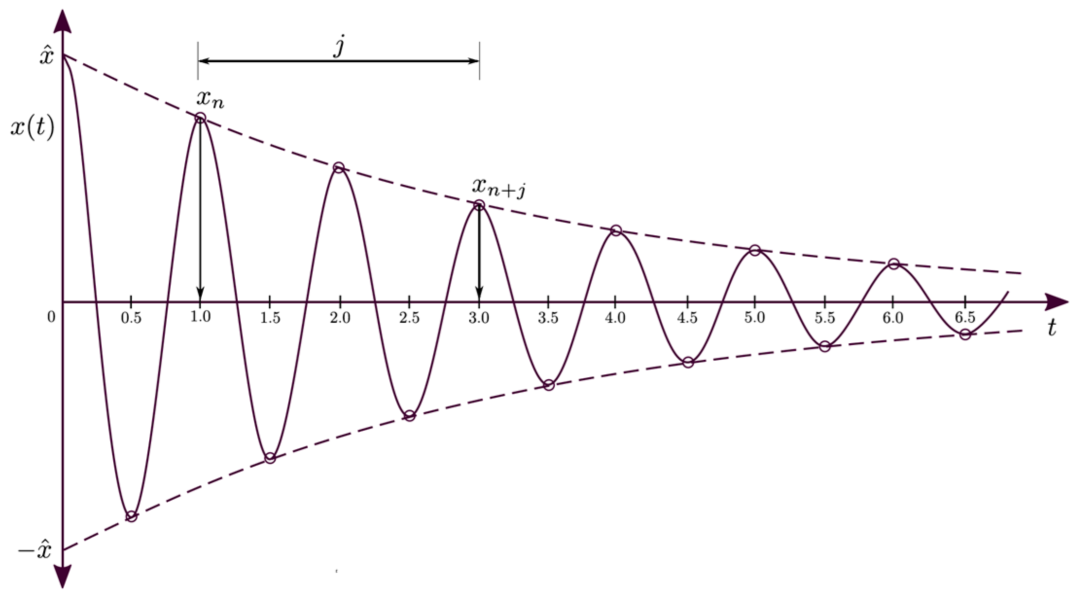
4.1. Logarithmic Decrement Method (LDM)

The logarithmic decrement method is a simple and widely used technique for determining the damping coefficient from a free vibration decay response. The log-decrement (δ) is defined as the logarithmic ratio between two consecutive peak amplitudes (x_n and x_n+j) in the free decay response, corresponding to the times t_n and t_n+j, as shown in Figure 2. The log-decrement can be expressed as

$$\delta =\frac{1}{j}ln\frac{x_n}{x_{n+j}}=\frac{2\pi \xi }{\sqrt{1-\xi }}$$

4.2. Hilbert Transform Method (HTM)

HTM is a well-known approach to identifying modal damping and the frequency of the SDOF of a system. The Hilbert transform is a linear time domain transformation that allows for a complex-valued representation of the analytical signal. The Hilbert transform, $\tilde{x}$(t), of a signal, x(t), can be represented as

$$\mathcal{H}\left[x\left(t\right)\right]=\tilde{x}\left(t\right)=\frac{1}{\pi }{\int }_{-\infty }^{\infty }\frac{x\left(\tau \right)}{t-\tau }d\tau$$

The analytical signal X(t) is

$$X\left(t\right)=x\left(t\right)+j\tilde{x}\left(t\right),(j=-1)$$

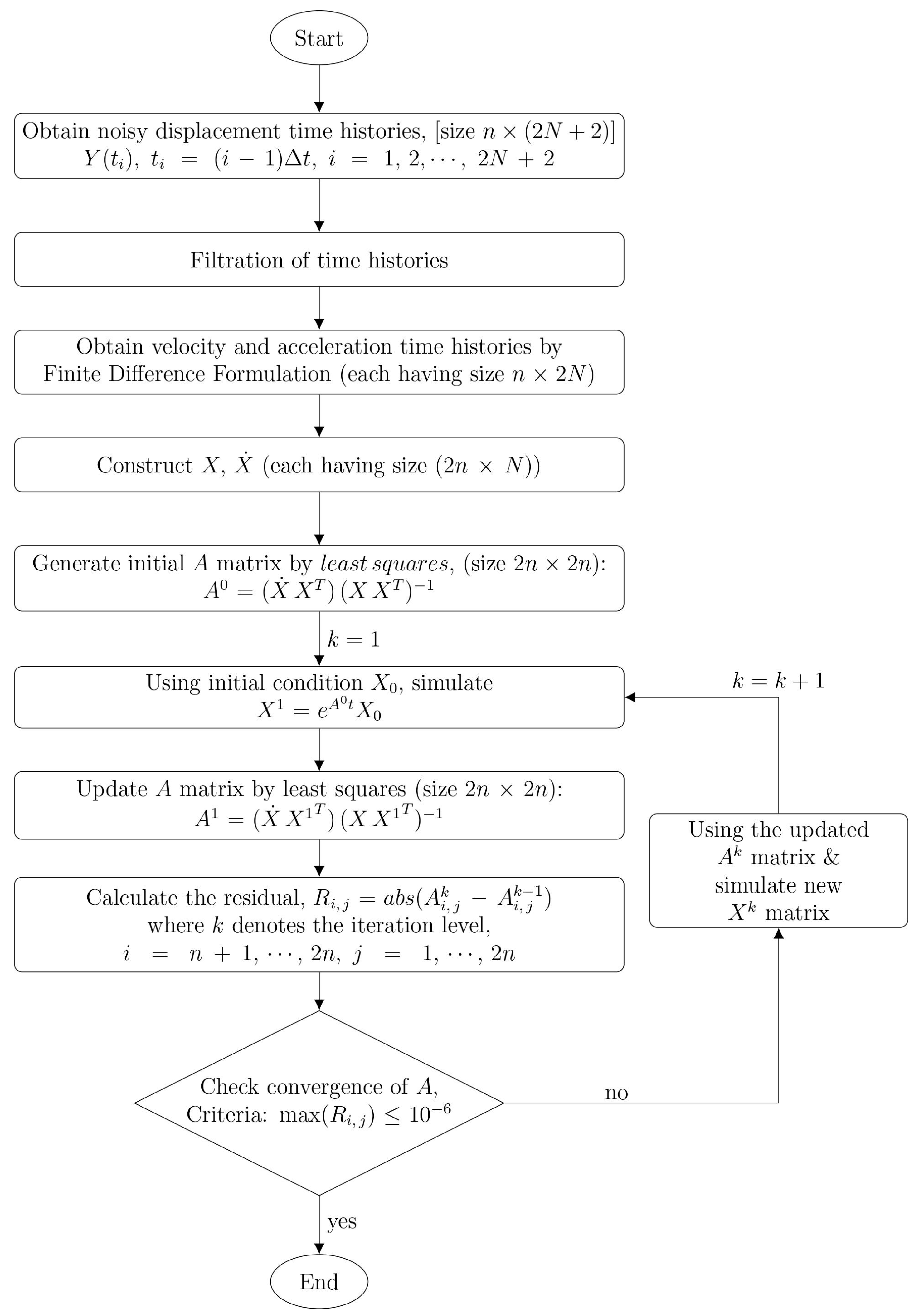
4.3. Iterative Least Squares (ILS)

Iterative least squares is a system identification method developed by Chowdhury and Sarkar [32] to extract flutter derivatives from free vibration tests. The fundamental idea behind this method is to obtain system matrix A using a state–space model from noise-corrupted time histories. Considering the two-degree-of-freedom system, the state–space model can be expressed as

$$\dot{X}=AX$$

$$\left[\begin{array}{c}\dot{h}\\ \dot{\alpha }\\ \ddot{h}\\ \ddot{\alpha }\end{array}\right]=\left[\begin{array}{cc}0& I\\ -K^{eff}& {-M}^{eff}\end{array}\right]\left[\begin{array}{c}h\\ \alpha \\ \dot{h}\\ \dot{\alpha }\end{array}\right];I=\left[\begin{array}{cc}1& 0\\ 0& 1\end{array}\right];0=\left[\begin{array}{cc}0& 0\\ 0& 0\end{array}\right]$$

Matrix A is a square matrix of the order 2n × 2n, where n is the number of degrees of freedom in the system. Matrix A can be identified if the acceleration, velocity, and displacement time histories are recorded for n degrees of freedom. The ILS method is preferred over other system identification methods due to its simplicity, as it does not require time shift parameters and directly identifies the system matrix without solving eigenvalue problems, reducing mathematical complexities. A flowchart of the ILS algorithm is shown in Figure 3.

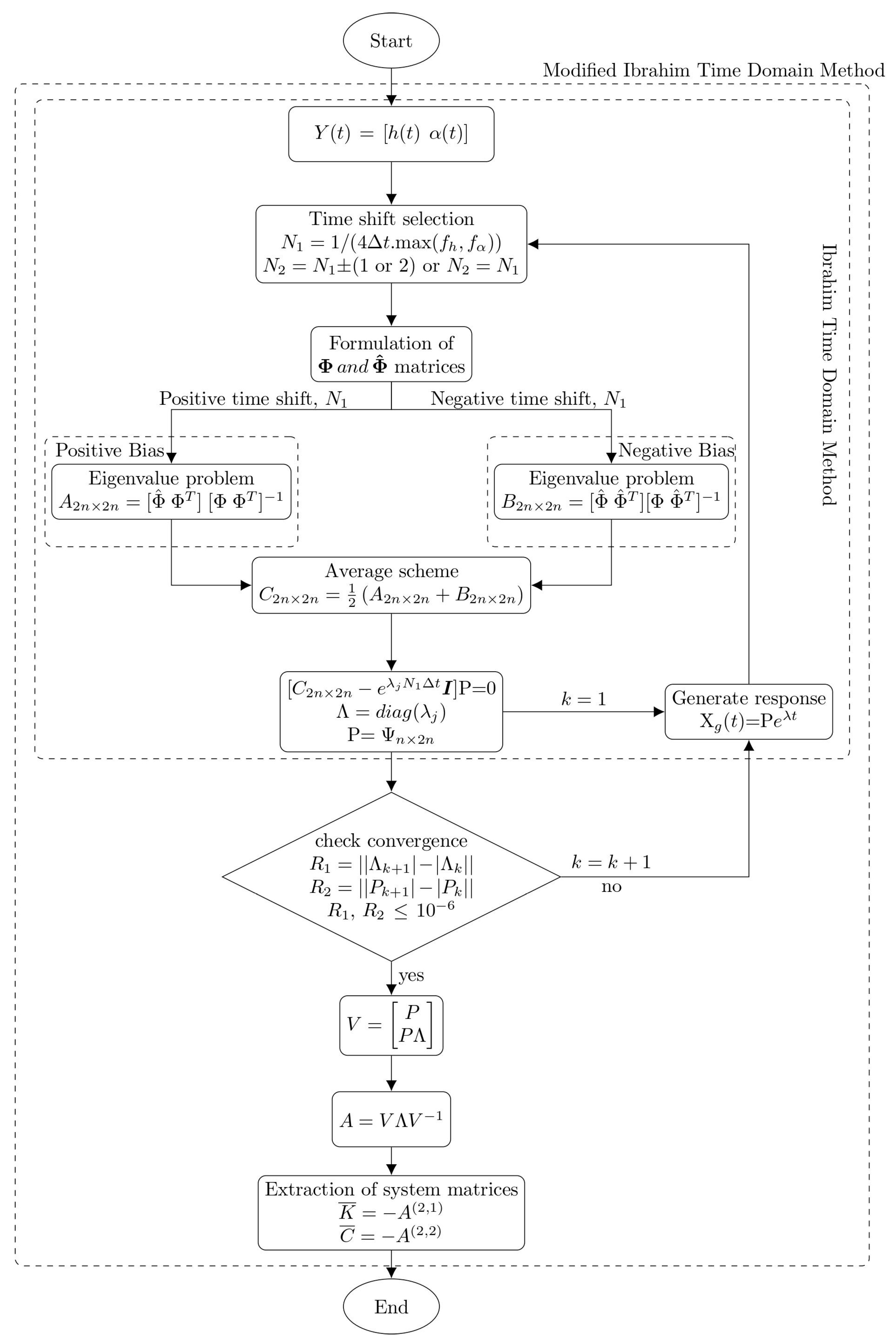
4.4. Modified Ibrahim Time Domain (MITD) Method

The MITD method, developed by Sarkar [34], is used to obtain flutter derivatives from bridge section free vibration wind tunnel tests. The equation of motion for the linear dynamic system can be written as

$$M\ddot{X}(t)+C\dot{X}(t)+KX(t)=F(t)$$

The current study aims to extract flutter derivatives in smooth flow conditions and considers any turbulence as additional noise. The modified Ibrahim time domain method uses the initial parameters determined by the ITD method. The MITD method can clean the noise-corrupted signal through an iterative process, and it accurately identifies the system parameters. A flowchart of the MITD algorithm is shown in Figure 4.

5. Experimental Program

The wind tunnel facility at Bauhaus-Universität Weimar was used to perform the free vibration tests for both the SDOF and 2DOF tests. The Great Belt Bridge, shown below in Figure 5, was chosen as a reference as it is a well-studied cross-section in bridge aerodynamics [35,36]. This bridge is one of the world’s longest and a notable engineering feat in Danish history, featuring a continuous girder without expansion joints. It connects the two Danish islands of Funen and Zealand with a main span of 1624 m and two side spans of 535 m each, helping to limit movement due to traffic and wind. The basic data and structural properties of the Great Belt Bridge are provided in

Table 1. Structural properties of the Great Belt Bridge [37].

Structural Parameter	Symbol	Value
Total span	lspan	2694 m
Deck width	B	31 m
Deck depth	D	4.4 m
Mass	M	22.74 t/m
Mass moment of inertia	I	2.47 × 103 tm2/m
First vertical frequency	fh	0.10 Hz
First torsional frequency	fa	0.78 Hz

, below. Some general arrangements of the bridge are shown in Figure 5.

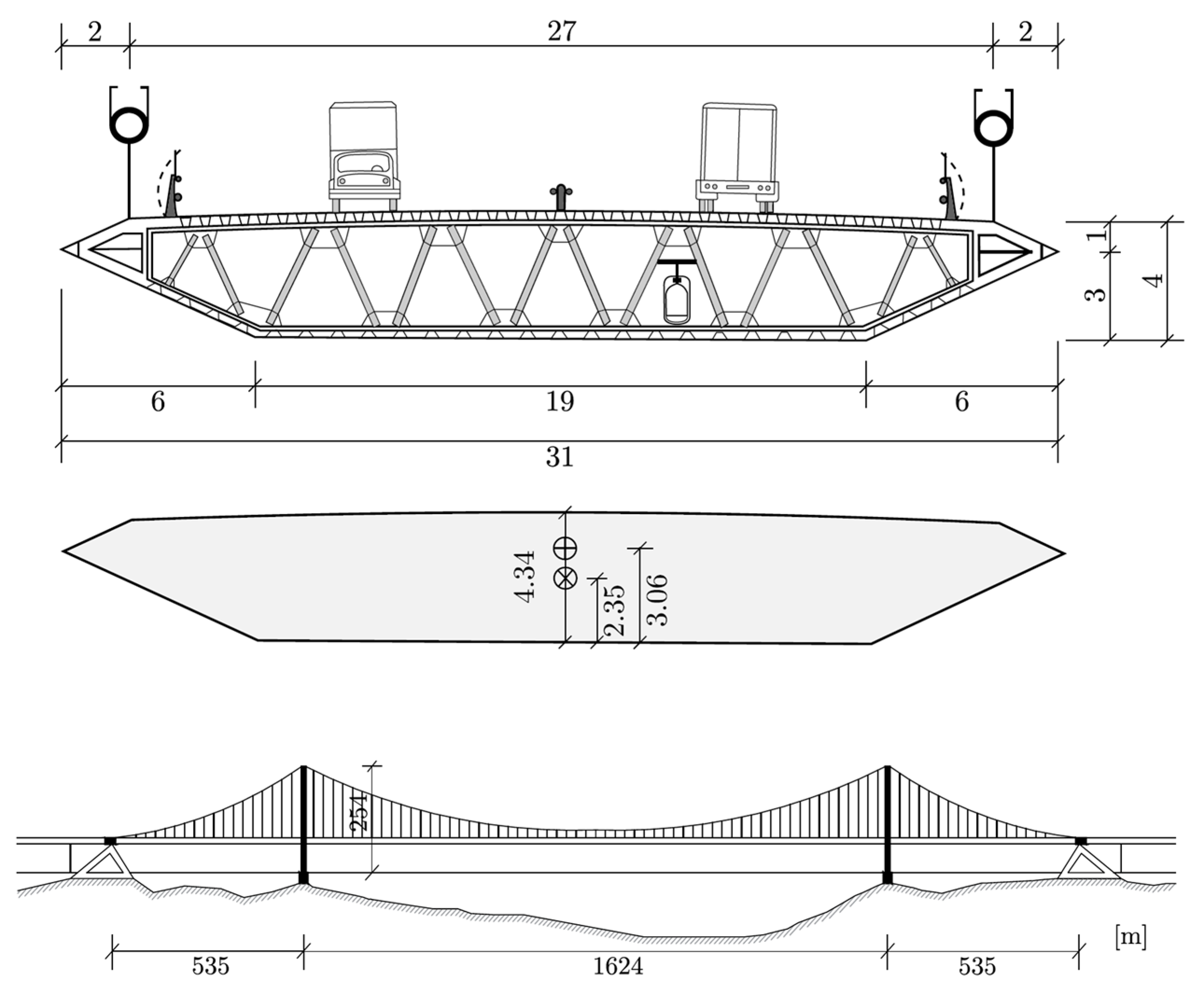
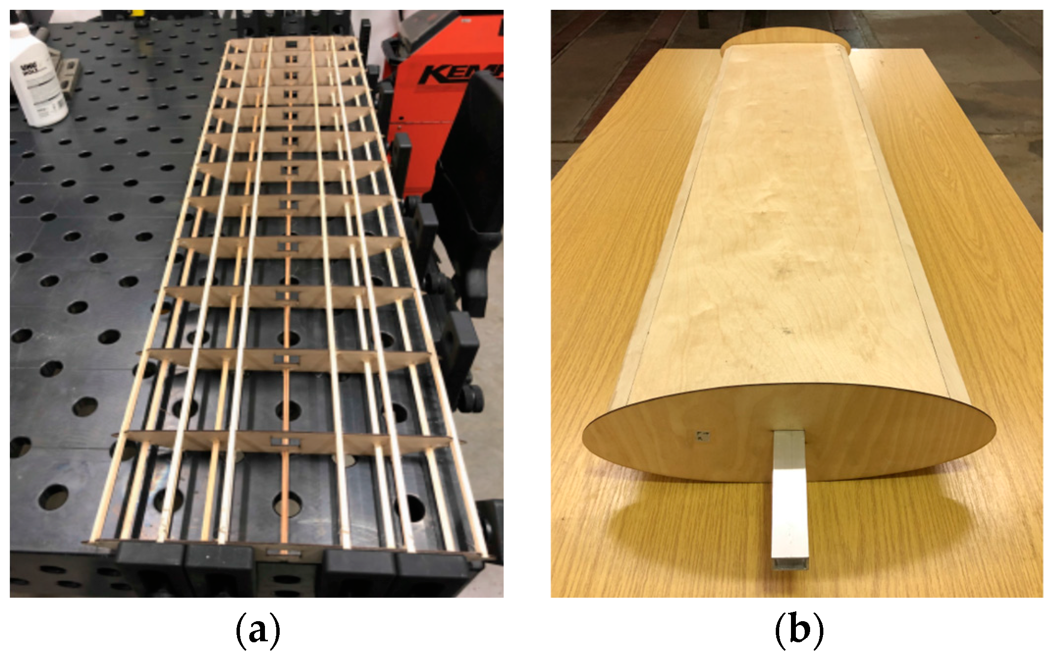
5.1. Bridge Section Model for Wind Tunnel Test

The reference section for the study was made from aircraft plywood and reinforced by eleven cross-sectional diaphragms. It was fitted with elliptical endplates to prevent aerodynamic end effects and maintain two-dimensional flow during testing. The section model had a length of 1.2 m, a width of 0.31 m, and a depth of 0.044 m, with a 1:100 geometric scale. Nonstructural details were not included in the model. The bridge cross-section and skeleton of the bridge deck model are shown in Figure 6.

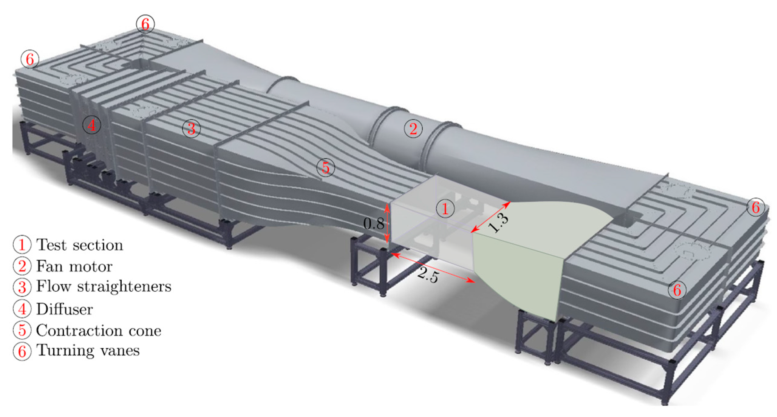
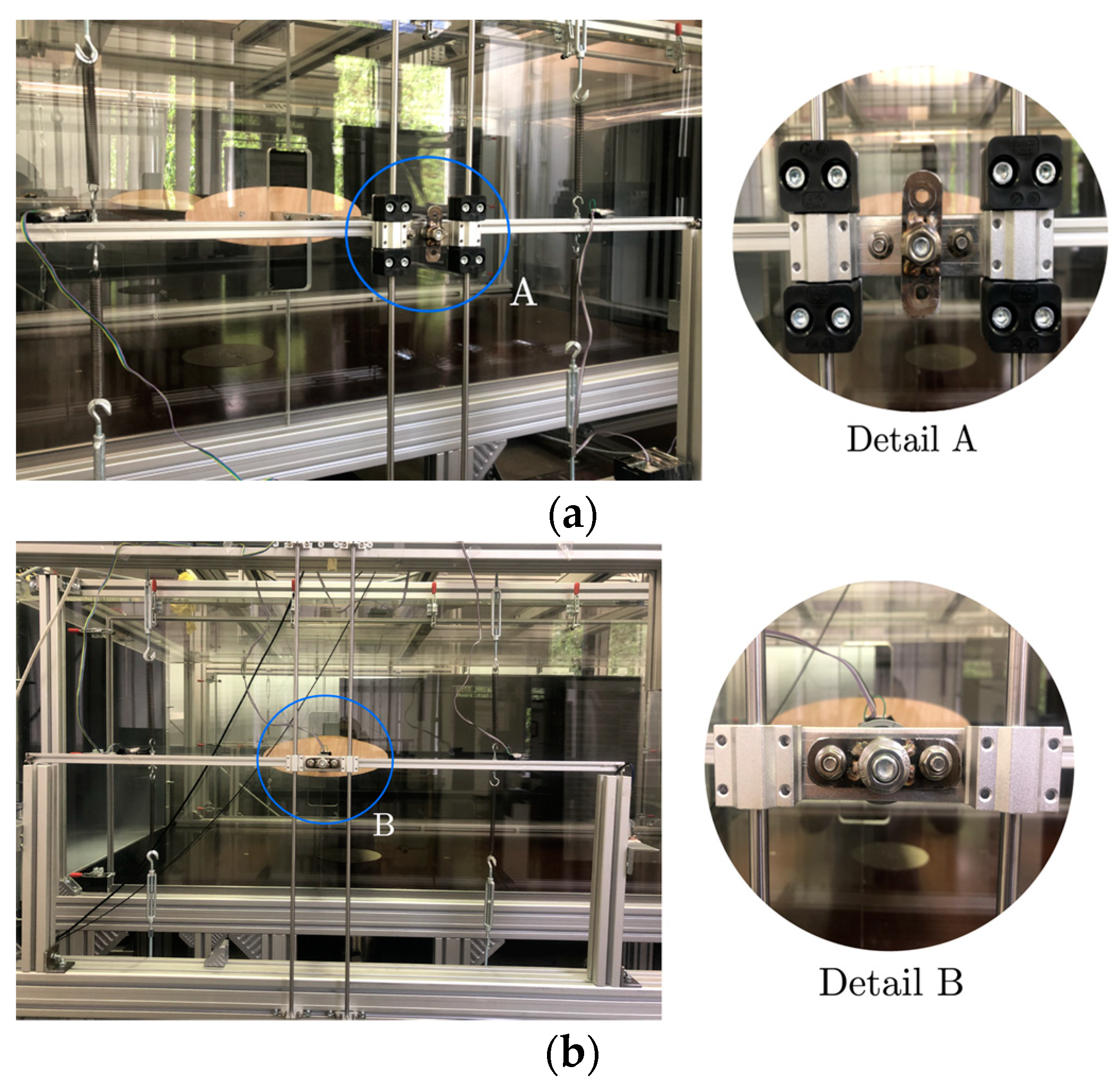
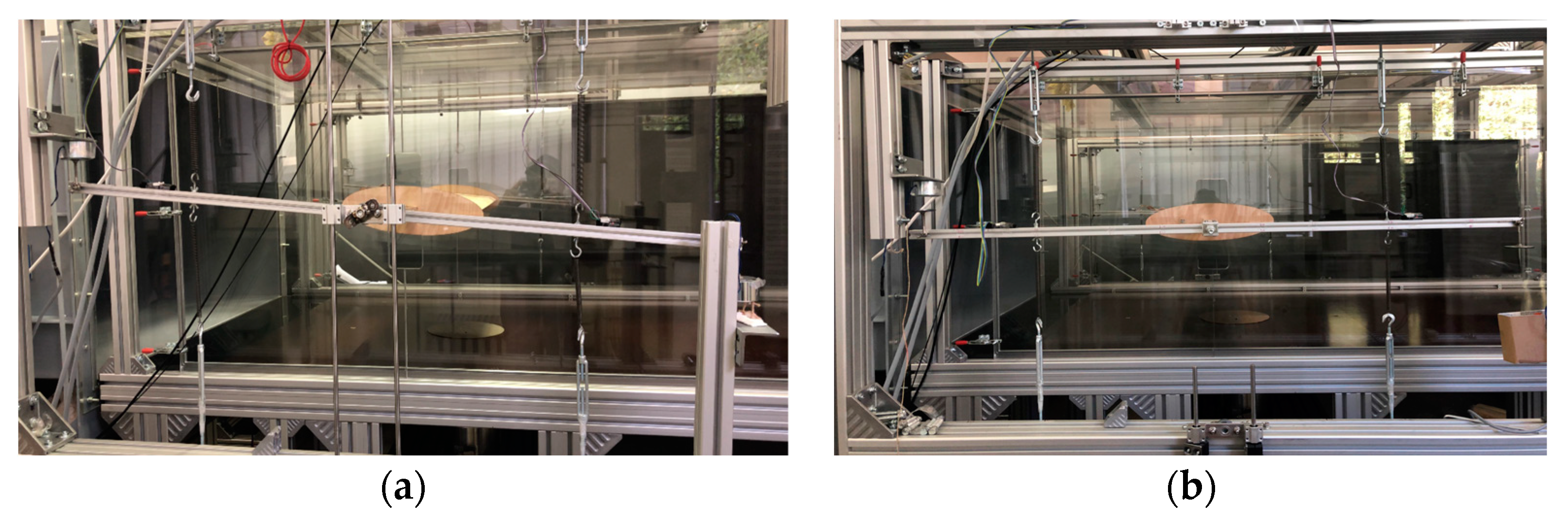
5.2. Bauhaus-Universität Weimar Wind Tunnel Facility

The free vibration tests were carried out in the wind tunnel facility at the Bauhaus-Universität Weimar. Figure 7 shows the 3D model of the wind tunnel facility at Bauhaus-Universität Weimar. The tunnel is a closed-loop and low-speed-type wind tunnel. This wind tunnel has a test section size capacity of 2.5 × 1.3 × 0.8 m (length × width × height). The allowable wind speed range is 1–30 m/s, and the provided degree of turbulence is 0.5% in the case of the closed measuring section and 0.8% in the case of the open measuring section.

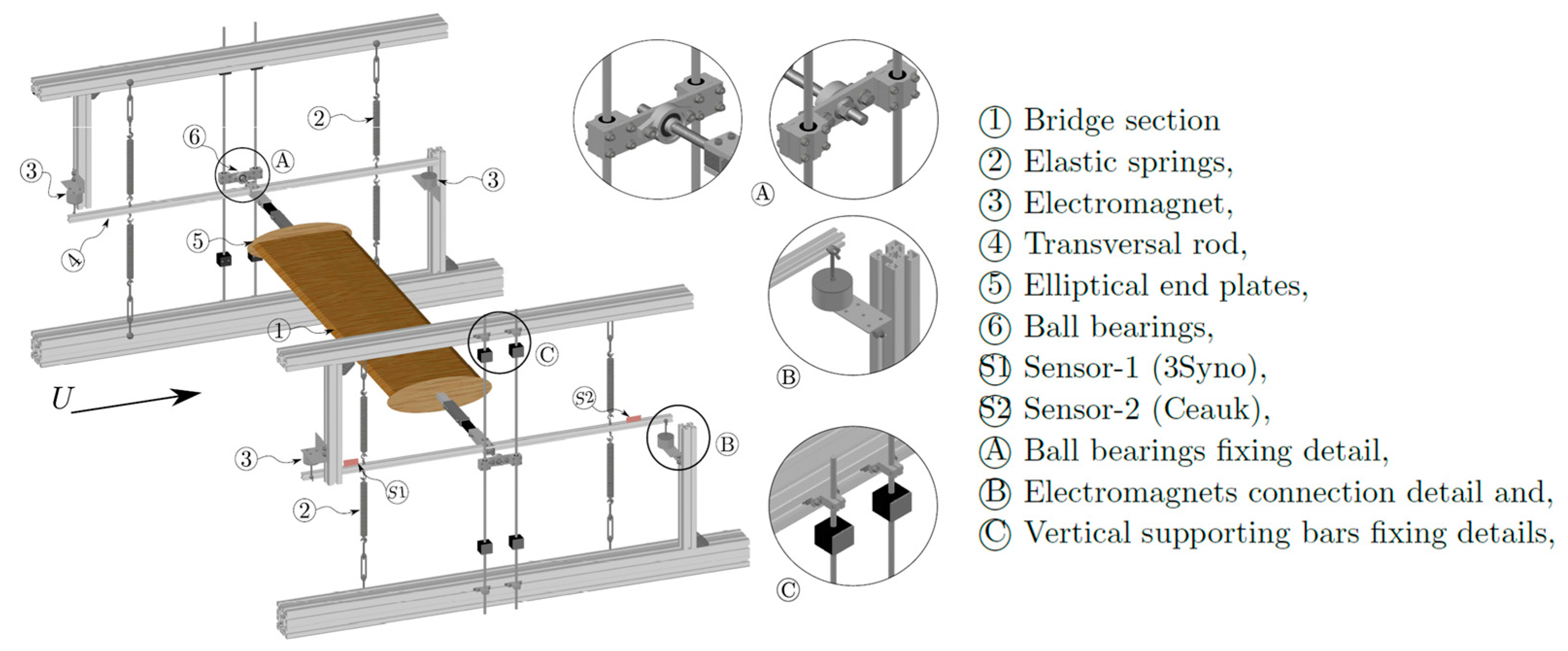
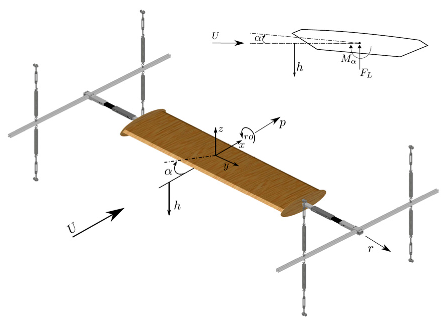
5.3. Free Vibration Test Setup Arrangement

The proper design and arrangement of the test setup are very important to achieve the desired motion. Conventional methods for sensor placement use structural characteristics to determine sampling positions, but they do not consider load cases or actual structural responses, which can lead to errors [40]. The initial stage of model updating to acquire the real structural response necessitates a well-designed sensor network with a suitable sensor arrangement [41]. In this research work, a novel free vibration test setup was designed to achieve vertical (h), torsional (α), and coupled motion in the section model. Figure 8 shows the 3D model of the test setup arrangement.

The test setup consists of a bridge section model with a T-shaped bar, “4”, fixed to an extended longitudinal bar using bolts. The assembly is supported vertically by eight external elastic springs, “2”, and we can control its torsional frequency by adjusting the spring spacing. Two vertical bars with brakes, Ⓒ, on either side allow for vertical adjustments and restrict motion along the longitudinal and wind directions. These rods also restrict the bridge deck motion along the longitudinal axis, r, as well as along the wind direction, p, as illustrated in Figure 9. The torsional adjustments are performed using the ball-bearing assembly, as shown in detail Ⓐ. There are four electromagnets, “3”, attached to the corners of the rig, Ⓑ, to precisely achieve controlled release conditions (h ≠ 0 and α ≠ 0). To record the vertical and torsional motion time histories, two sensors, “S1” and “S2”, are attached to the transversal rod. Precise control of the initial conditions is important to avoid nonrepresentative free-decay motion, and initial conditions are determined by the desired degrees of freedom to be excited by the top of the form:

(h ≠ 0, α = 0; h = 0, α ≠ 0; h ≠ 0, α ≠ 0).

5.4. Test Setup Assembly

5.4.1. Single-Degree-of-Freedom Assembly

The SDOF torsional motion was triggered by restricting the vertical DOF (h = 0) using brakes, as shown in Figure 10. A circular ball bearing connected to the section axis via a solid circular shaft and an adjustable steel plate controlled the torsional fixity. The four elastic springs connected to the transversal bar produced the oscillatory motion. One electromagnet was inverted on either side of the section to maintain proper initial torsional displacement. Pure vertical motion was generated by removing the brakes and fully tightening the plate, restricting the torsional DOF (α = 0). The initial vertical displacement was controlled by equalizing all magnets. A misalignment of the top and bottom horizontal supporting frames disturbed the smooth movement of the vertical bearings, causing additional noise. Adjusting the top and bottom connection of the vertical bars with washers was the solution.

5.4.2. Two-Degree-of-Freedom Assembly

Two-degree-of-freedom tests were conducted using two testing arrangements. In Setup 1, as shown in Figure 11a, all components from the SDOF vertical and torsional tests were used. The 2DOF motion was achieved by removing the restraints for both DOFs. This setup had the disadvantage of additional noise from the vertical bearings, but this was improved by greasing the vertical bearings and bars before the experiment. In Setup 2, as shown in Figure 11b, the vertical bars and torsional and vertical bearing assemblies were removed to eliminate the issue of additional noise from vertical bearings but introduced unwanted motions such as rocking of section, r_o; horizontal displacement, r; and displacement, p, along the wind direction, as shown in Figure 9.

6. Experimental Procedure

The following procedure was adopted for the free vibration test:

■

Check and adjust the horizontal position of the section model to zero angles of attack.

■

Displace the section vertically, torsionally, or both using electromagnets.

■

Generate wind flow of the desired velocity using a fan motor (range 0–20 m/s).

■

Record vertical and torsional response of the section using accelerometers.

■

Release the section and record the acceleration response until the motion is damped.

■

Repeat the procedure for each experiment. The rotation angle is measured before releasing the section at higher wind speeds; the section experiences static aerodynamic moment, which can cause deflection in the section.

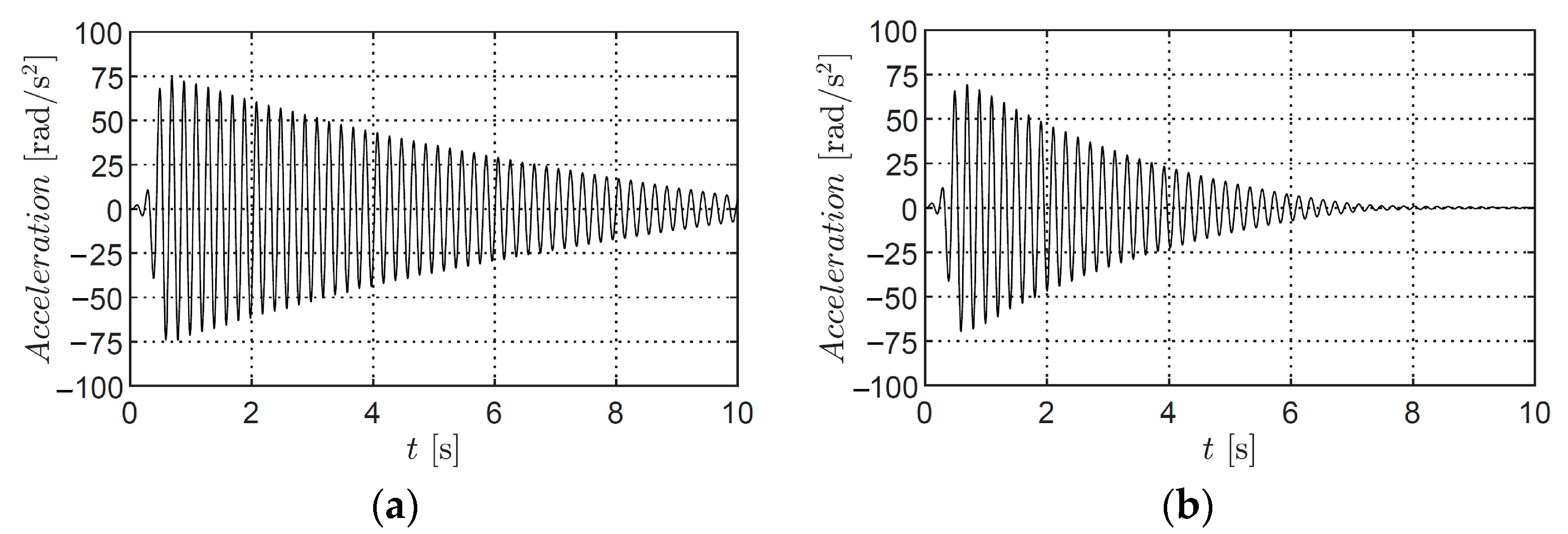
7. Signal Processing:

7.1. Single-Degree-of-Freedom Acceleration Response

Signal conditioning was applied before analyzing the deck response with the SID algorithm to extract useful information and reduce noise. The deck response was recorded as an acceleration time history using accelerometers at the ends of the bars, but the recorded response had a lot of noise, including system noise and mechanical noise from wind tunnel vibrations at high speeds. Figure 12 shows the deck response for SDOF heave and pitch at wind speeds of 0 m/s and 10 m/s.

Noise affects the response more at high wind speeds due to increased wind tunnel vibrations. The initial cycles contain extra modes due to the catapult effect. The pitch response at zero wind speed shows clean harmonics after the initial cycles, but the heave response has noise even at zero wind speed, possibly caused by friction in the bearings. The response was resampled, normalized, and conditioned by removing the mean and applying a lowpass filter at 10 Hz and a Butterworth band pass at 2 Hz and 6 Hz to remove noise and produce clean time histories. The dominant heave frequency was 3 Hz, and the pitch was 5 Hz, with high-frequency noise at 40 Hz. The filtered response of the heave and pitch motion is shown in Figure 13. The signal conditioning produced clean and smooth time histories that were used to identify SDOF parameters for heave and pitch motions.

7.2. Single-Degree-of-Freedom Displacement Response

The system parameters were also identified using the displacement response, as the system was released from a known initial displacement that was easily identifiable from the response. The displacement response was obtained by integrating the filtered acceleration data twice and removing DC components and numerically generated noise with detrending and filtering at each step. The initial displacement values for vertical and torsional degrees of freedom can be found from the initial data points of the time histories, as shown in Figure 14.

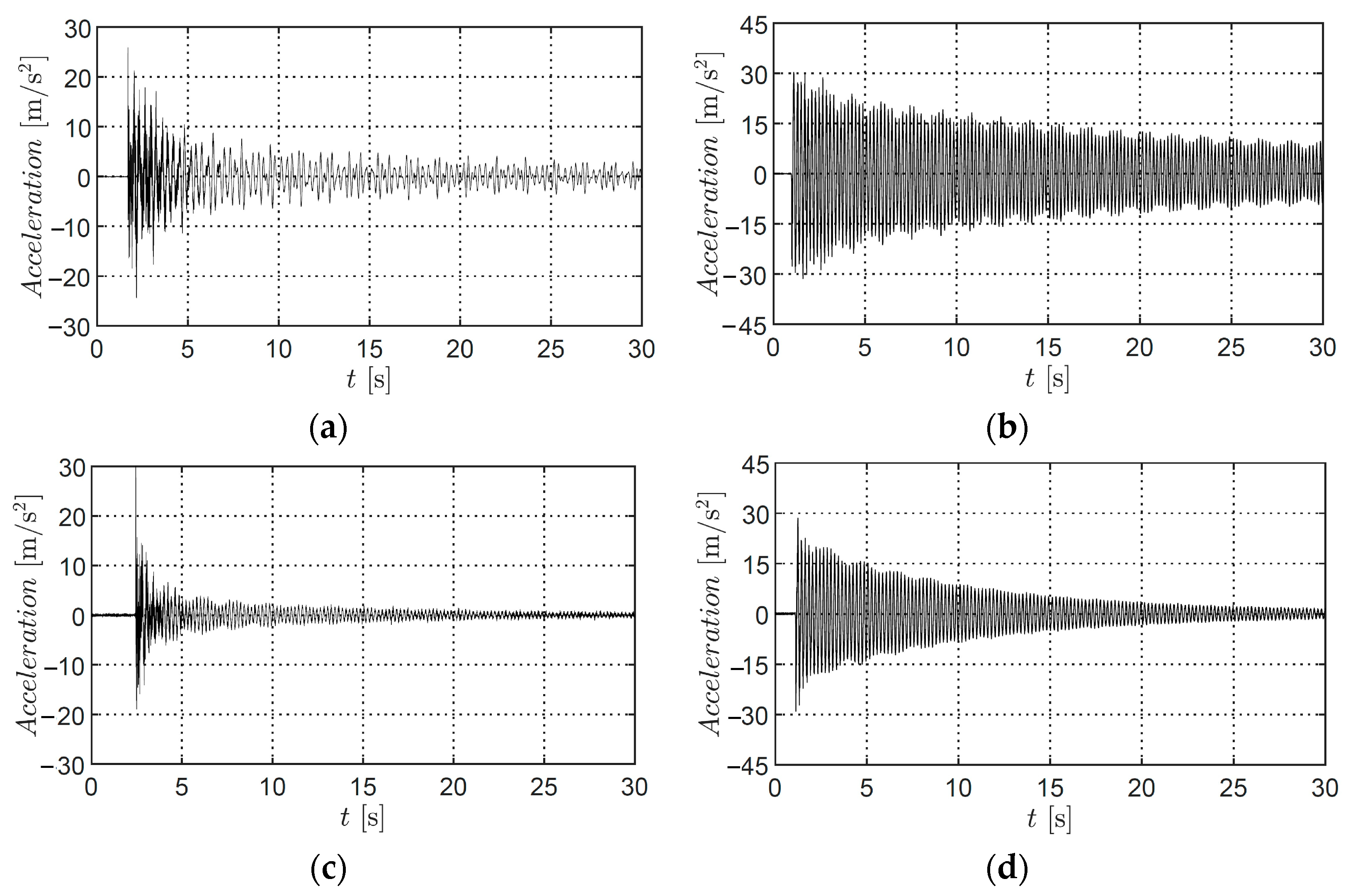
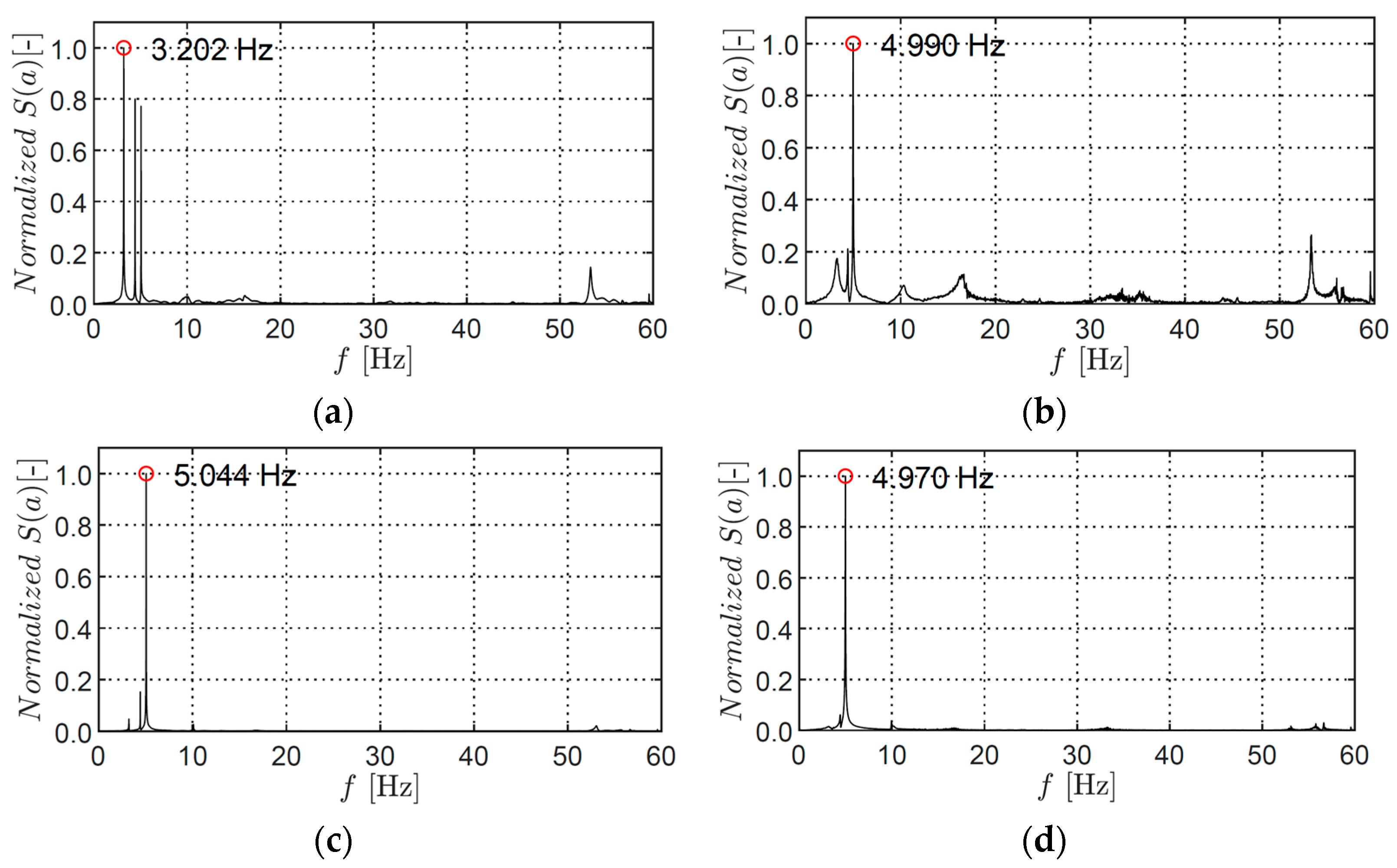
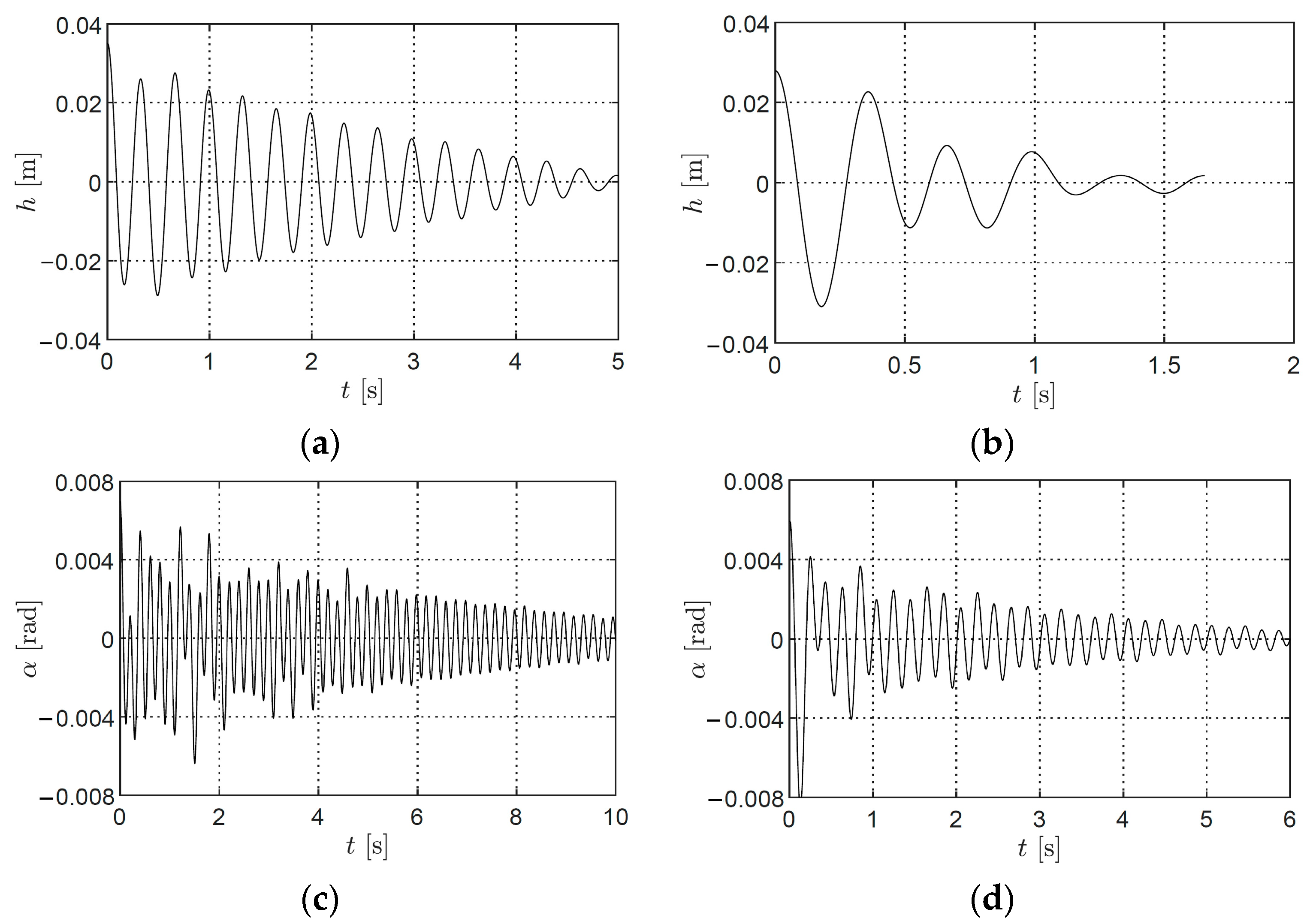
7.3. Two-Degree-of-Freedom Acceleration Response

The 2DOF acceleration response was obtained using the same sensor setup as the SDOF tests, allowing the bridge section to oscillate in both vertical and torsional DOF. Two setups were prepared for 2DOF experiments, and two testing arrangements were considered to record the coupled motion. The first arrangement was with initial displacement in the vertical DOF (called “vertical-dominant coupled motion”), and the second was with initial displacement in the torsional DOF (called “torsional-dominant coupled motion”). The acceleration responses for the 2DOF tests for both vertical- and torsional-dominant motions are shown in Figure 15. The response dampened faster at 10 m/s wind speed than at 0 m/s due to added aerodynamic damping from the wind flow on the section.

The FFTs of the vertical- and torsional-dominant motions are plotted in Figure 16 in which red circle shows the peak value. The vertical-dominant motion has more noise contributions compared with the torsional-dominant motion. At 10 m/s, the high-frequency noise overshadowed the vertical-dominant frequency.

Similarly, vertical- and torsional-dominant responses from Setup 2 are shown in Figure 17. The corresponding frequency spectrum is shown in Figure 18 in which red circle shows the peak value.

The vertical-dominant response from Setup 1 was more affected by noise than Setup 2, indicating that the vertical bearings were a major source of noise. The torsional-dominant responses from both setups were less affected by noise. The vertical- and torsional-dominant responses from Setup 1 decayed regularly, while those from Setup 2 decayed irregularly, possibly due to the presence of unrestricted rocking motion. The frequency spectrum analysis of Setup 2 responses showed three dominant modes at 0 m/s wind speed, with the frequency of 3.202 Hz representing the vertical mode, 5.04 Hz the torsional mode, and 4.41 Hz the unrestricted motion, which was more prominent in the vertical dominant response. The FFT of the torsional-dominant response from Setup 1 showed no contribution from the vertical mode, while the FFT of the torsional dominant response from Setup 2 showed a small peak representing the vertical frequency.

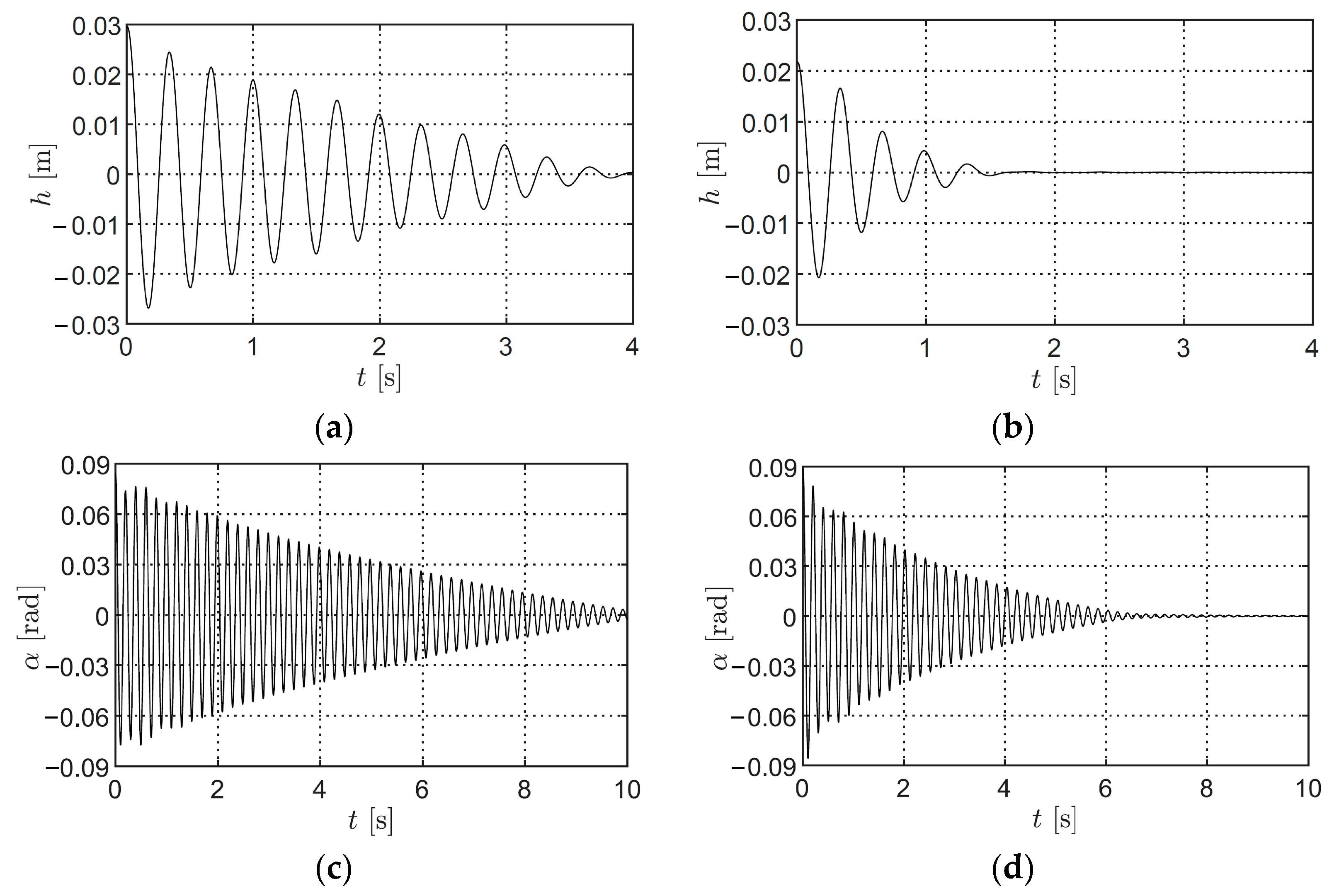
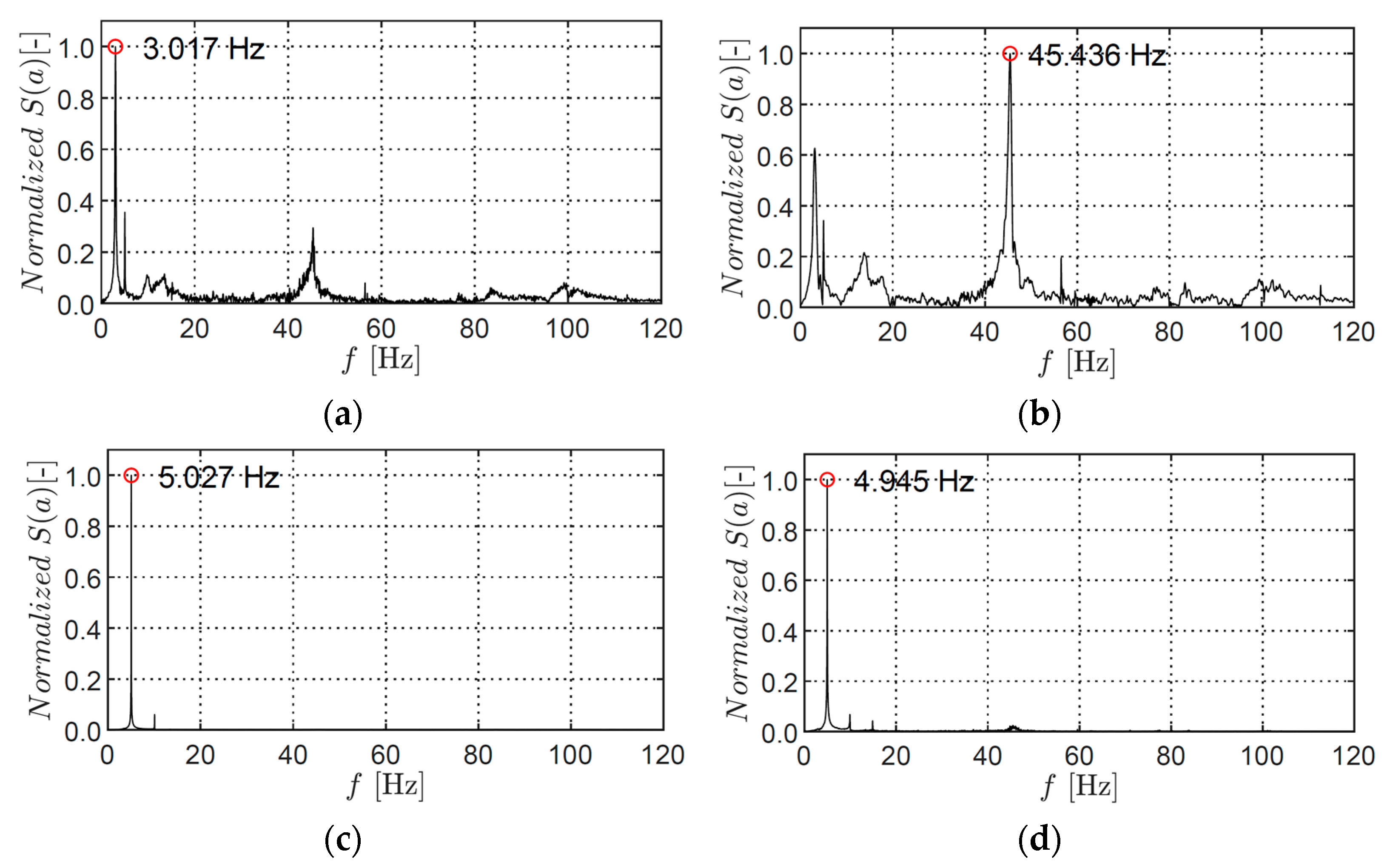
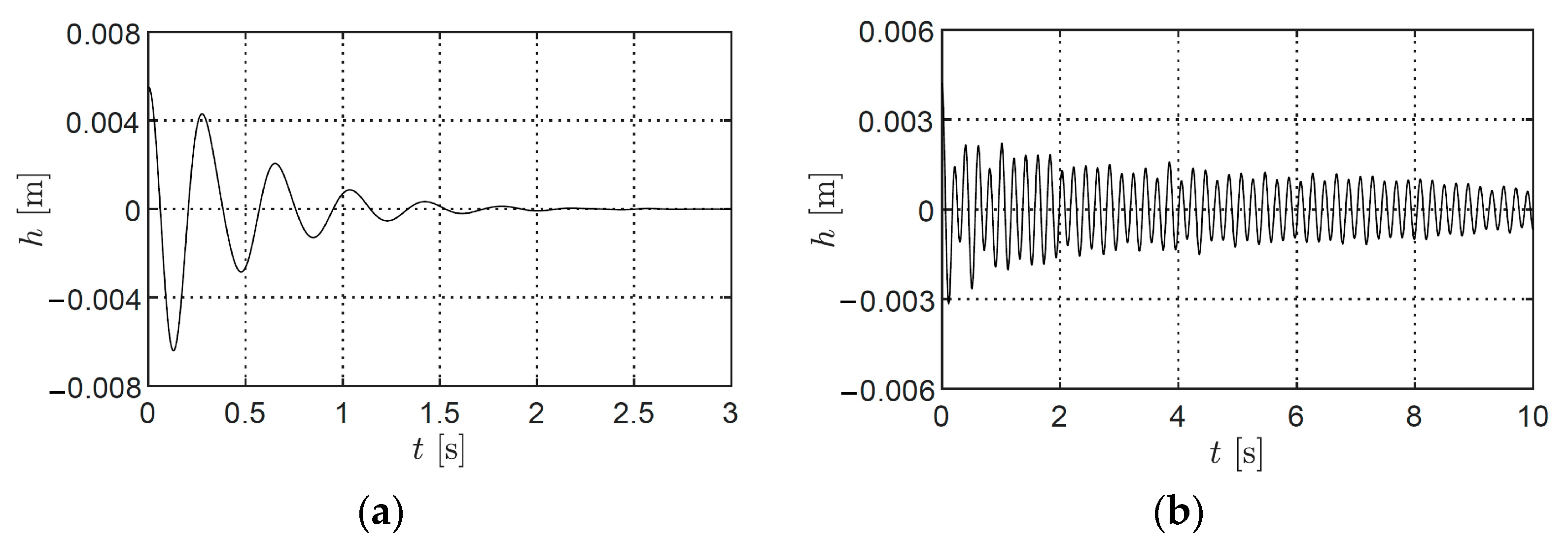
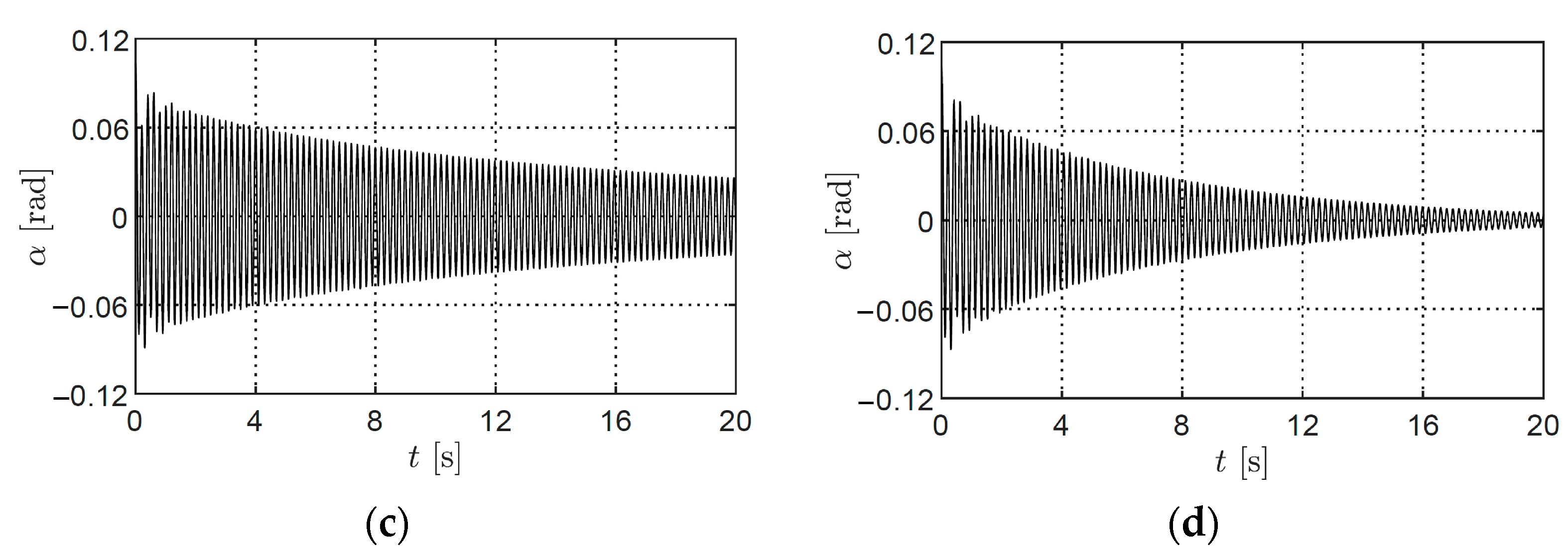
7.4. Two-Degree-of-Freedom Displacement Responses

The system identification methods for 2DOF require displacement responses. The raw responses were converted to displacement by first filtering out high-frequency noise and then integrating twice. The dominant frequencies for vertical and torsional responses were 3.01 Hz and 5.02 Hz, respectively, for Setup 1 and 3.202 Hz and 5.04 Hz, respectively, for Setup 2. A band-pass filter with lower and upper cut-off limits of 2 Hz and 6 Hz was used. Vertical displacement was obtained by averaging the two sensors, while torsional displacement was based on the sensor position. For Setup 1, the extracted vertical and torsional displacement responses from the vertical-dominant coupled response are presented in Figure 19, and the torsional-dominant responses are in Figure 20. Similar responses were generated for Setup 2.

8. Results and Discussions

Identification of Stiffness and Damping

The stiffness of SDOF was determined after extracting the frequency and by using the expression $K_h=m{w}_h^2$ for heave and $K_{\alpha }=m{w}_{\alpha }^2$ for pitch. The damping values were obtained using the logarithmic decrement method (LDM), the exponential decay curve fitting method, and the Hilbert transform method for both the heave and pitch responses, as shown in Figure 21. For the heave response, a good agreement can be observed between the polynomial fit of the exponential decay curve and the Hilbert transform. On the contrary, a better match can be seen between the Hilbert transform and the LDM values in the case of the pitch. The corresponding frequency values of the HT are presented in Figure 22.

9. Identification of Flutter Derivatives from SDOF Tests

The flutter derivatives for vertical ($H_1^{*}$ and $H_4^{*}$) and torsional ($A_2^{*}$ and $A_3^{*}$) DOFs were extracted from the SDOF heave and pitch vibration responses. The basic experimental parameters used for SDOF testing and the calculation of flutter derivatives are listed in

Table 2. Experimental parameters for wind-off case from SDOF test.

B (m)	mh (kg)	Iα (kgm2)	fh (Hz)	fα (Hz)	$\mathit{\rho }$ * kg/m3	ξh (%)	ξα (%)
Logarithmic Decrement Method
0.31	4.348	0.0906	3.022	5.028	1.145	2.208	0.738
Exponential Curve Decay Method
0.31	4.348	0.0906	3.022	5.028	1.145	2.216	0.567
Hilbert Transform Method
0.31	4.348	0.0906	3.021	5.030	1.145	2.670	0.698

* Air density is at 22.5°, 0.976 bars, and 40.4% relative humidity.

. The initial displacements given in the vertical and torsional DOFs were h₀ = 4 cm and α₀ = 5°, respectively. The required mechanical and effective system parameters were obtained from wind-off and wind-on responses. The obtained direct flutter derivatives are plotted in Figure 23 and Figure 24. Additionally, these derivatives are compared with the flat plate derivatives and the derivatives obtained from the selected wind tunnel studies [2,42] on the Great Belt section. It is important to mention that the derivates obtained from the literature are manually digitized and, therefore, subject to uncertainties.

9.1. Flutter Derivatives Using the Hilbert Transform Method, Logarithmic Decrement Method, and Exponential Decay Curve Method

The derivatives obtained using Hilbert transform and logarithmic decrement methods and by using the polynomial fit of exponential decay curve are shown in Figure 23. The $H_1^{*}$ derivative does not show good agreement with the reference experimental results but shows quite good agreement with the flat plate at low reduced wind speeds, whereas $A_2^{*}$ illustrates a good correspondence with the reference experimental results. Overall, both derivatives ($H_1^{*},A_2^{*})$, computed from different methods, demonstrate a similar trend. Additionally, $A_3^{*} \mathrm{and} H_4^{*}$ derivatives obtained from HTM show close correspondence with the reference experimental values. The $A_2^{*}$ and $A_3^{*}$ have similar results in all three methods but have a shift in values when compared with the flat plate by Theodorsen.

9.2. Flutter Derivatives Using the MITB and ILS Methods

The derivatives obtained using the modified Ibrahim transform and ILS methods are shown in Figure 24. The accuracy of the derivatives and effectiveness of different methods can be improved by performing repeated wind tunnel tests. A good agreement can be seen between the coefficients obtained using the MITD and ILS methods. These derivatives also show good correspondence with the theoretical and reference experimental results. The $H_4^{*}$ values show a large scatter after a reduced velocity of 10 m/s, which can be related to the different stiffness and frequency values.

10. Identification of Flutter Derivatives from 2DOF Tests

All eight flutter derivatives were calculated using the MITD and ILS method in two configurations (Setup 1 and Setup 2). The parameters used to compute the derivatives from the 2DOF tests are listed in

Table 3. Experimental parameters for wind-off case from 2DOF tests.

B (m)	mh (kg)	Iα (kgm2)	fh (Hz)	fα (Hz)	$\mathit{\rho }$ * kg/m3	ξh (%)	ξα (%)
Test Setup 1
0.31	4.348	0.0906	3.017	5.027	1.145	1.83	0.22
Test Setup 2
0.31	3.825	0.1256	3.202	5.044	1.145	1.75	0.49

* Air density is at 22.5°, 0.976 bars, and 40.4% relative humidity.

. The wind speed was calculated using the still-air heaving frequency, and heave and torsional frequencies were used to calculate heave- and torsion-dependent derivatives, respectively. The initial conditions imposed on Setup 1 and Setup 2 vertically and torsionally were h₀ = 4 cm and α₀ = 5° and h₀ = 2 cm and α₀ = 3°, respectively.

10.1. Flutter Derivatives from MITD Method

The flutter derivatives obtained from the MITD method used filtered acceleration data from both Setups 1 and 2. Initially, raw acceleration data were used, but high-frequency noise and short data length at high wind speeds caused the MITD to produce a singular matrix, making it impossible to simulate time histories. The shifted response matrices were calculated using a fixed time shift, and the mechanical stiffness and damping matrices were extracted for both setups but showed non-zero off-diagonal values, which indicate a mechanical coupling between modes, which is unexpected at zero wind speed. This could be caused by the poor quality of the recorded data, which was shorter in the heave mode, or by small, unmeasured vertical displacements during the pitch-dominant motion. The extracted modal parameters, such as frequency and damping, also showed discrepancies, indicating the recorded data are of poor quality, as shown in Figure 25. These discrepancies can cause large errors in the flutter derivatives, making it important to accurately identify the mechanical parameters of the system. The MITD method itself is not responsible for the discrepancies. The mechanical stiffness and damping matrices extracted from the MITD method for both Setup 1 and Setup 2 are presented in

Table 4. Mechanical system matrices for wind-off conditions from the MITD method.

Motion	Stiffness Matrix		Damping Matrix
Setup 1	$\overline{K}$		$\overline{C}$
Heave-Dominant	361.09	−0.8605	0.698	−0.0421
	−11.517	984.73	0.1694	0.1783
Pitch-Dominant	491.62	0.4308	0.2169	−0.0099
	1036.9	9928.83	−31.79	0.1751
Setup 2	$\overline{K}$		$\overline{C}$
Heave-Dominant	454.06	−3.61	0.2117	−0.0896
	−13.63	1011.6	0.1871	0.174
Pitch-Dominant	698.76	1.078	0.9287	−0.0614
	4.947	1003.8	0.1224	0.0734

.

The flutter derivatives obtained using the MITD method from the 2DOF test in Setup 1 are shown in Figure 26 and are compared with the wind tunnel tests of reference studies. The results indicate that the $H_3^{*}$, $A_2^{*}$, and $A_3^{*}$ fitted derivatives from both dominant motions show good correspondence with each other. On the other hand, $A_1^{*}$, $A_4^{*}$, and $H_1^{*}$ show the same pattern but with large differences in values. $H_4^{*}$ coefficient values from both dominant motions show disagreement with each other. Overall, the fitted derivatives from both heave- and pitch-dominant motions show well-defined patterns, and their values are fairly close to the reference wind tunnel and water channel values.

The flutter derivatives obtained using the MITD method from the 2DOF test for Setup 2 are shown in Figure 27. The derivative values obtained from the heave-dominant motions show a large scatter as compared with the pitch-dominant motions. The large discrepancies can be linked to the bad quality of the recorded data that were used to calculate the mechanical parameters. The $A_1^{*}$ values from the pitch-dominant motions show good agreement with the experimental reference values. Overall, for Setup 2, the obtained derivatives from the pitch-dominant motions show a similar trend to those depicted by theoretical and experimental values.

10.2. Flutter Derivatives from ILS Method

The ILS method computes flutter derivatives using numerically obtained displacement, velocity, and acceleration responses. However, the properties of these responses may differ from the actual recorded responses due to filtration. The computed mechanical stiffness and damping matrices may also be affected.

Table 5. Mechanical system matrices for wind-off conditions from the ILS method.

Motion	Stiffness Matrix		Damping Matrix
Setup 1	$\overline{K}$		$\overline{C}$
Heave-Dominant	−360.567	5.885	−0.8407	−0.3517
	18.667	−979.77	−0.5524	−0.6884
Pitch-Dominant	−461.608	−0.7175	−3.731	0.0305
	969.21	−978.34	−75.761	−0.0806

presents the extracted system parameters from the ILS method in wind-off conditions, which show non-zero off-diagonal values for both heave- and pitch-dominant motions, indicating strong mechanical coupling between both motions. The ILS algorithm failed to simulate the response for Setup 2 due to convergence failure in matrix A or failure to identify the dominant motion in the response. This was likely due to the system’s flexibility causing an additional mode to be excited. Figure 28 shows all the obtained derivatives, which are compared with the theoretical and experimental reference values. The $H_1^{*}$ values from the heave-dominant motions show very close agreement with the reference experimental values. On the contrary, $H_1^{*}$ values from the pitch-dominant motions follow the same trend, but the values are not close to the theoretical or experimental values. The $H_2^{*}$ coefficients from both motions show the same trend, but the one from the pitch-dominant motions shows good correspondence with the water channel values and wind tunnel values obtained by Ge et al. [2]. Similarly, the $H_3^{*}$ values from both motions show the same decreasing trend as the reference values. In the case of $H_4^{*}$, a completely opposite trend is observed compared with the reference values. The $A_1^{*}$, $A_2^{*}$, and $A_4^{*}$ values from heave-dominant motions are in close agreement with the reference values. For the $A_2^{*}$ function, a close correspondence can only be observed at low reduced wind speeds with the reference values. In the case of pitch-dominant motion, a good agreement can be seen for $A_3^{*}$ and, similarly, for $A_2^{*}$ at low reduced wind speeds. The $A_2^{*}$ values become positive for reduced velocity above six, which indicates an increase in the damping values of the torsional motion. All the other derivatives of $A_1^{*}$ and $A_4^{*}$ show complete disagreement with the reference values. Overall, the derivatives computed for the heave-dominant response from the Setup 1 configuration show better results as compared with the pitch-dominant motions.

11. Numerical Identification of Flutter Derivatives Using VXFlow

The aerodynamic derivatives of the reference object are computed through forced vibration simulations in VXFlow. The section is driven into a heave and pitch motion with a predefined amplitude and oscillation frequency. The aerodynamic derivatives are obtained from the least squares fit of the lift and moment time histories. The numerical simulations were performed with defined flow properties, grid domain size, and section properties using the VXFlow solver. The section geometry was created and discretized into panels. The time step was calculated based on the panel size, and a 30 s stabilization time was added to ensure particle saturation. The simulations were run for heave and pitch motion over a range of reduced velocities, and the results were processed using the VXPost tool. The final computed flutter derivatives were compared to analytical flat plate values and showed good correspondence except for $A_4^{*}$. The sign of $H_2^{*}$ changed to positive at reduced velocities above V_r = 10, indicating classical flutter. The uncertainty in the results can be reduced by varying the numerical parameters. All eight flutter derivatives obtained from the CFD simulation are shown in Figure 29.

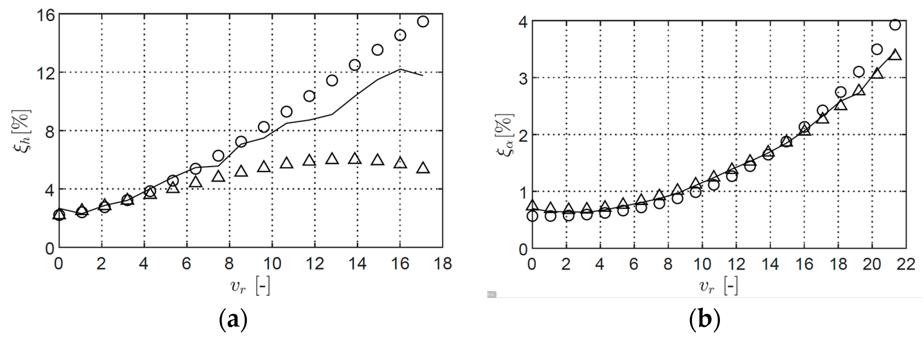
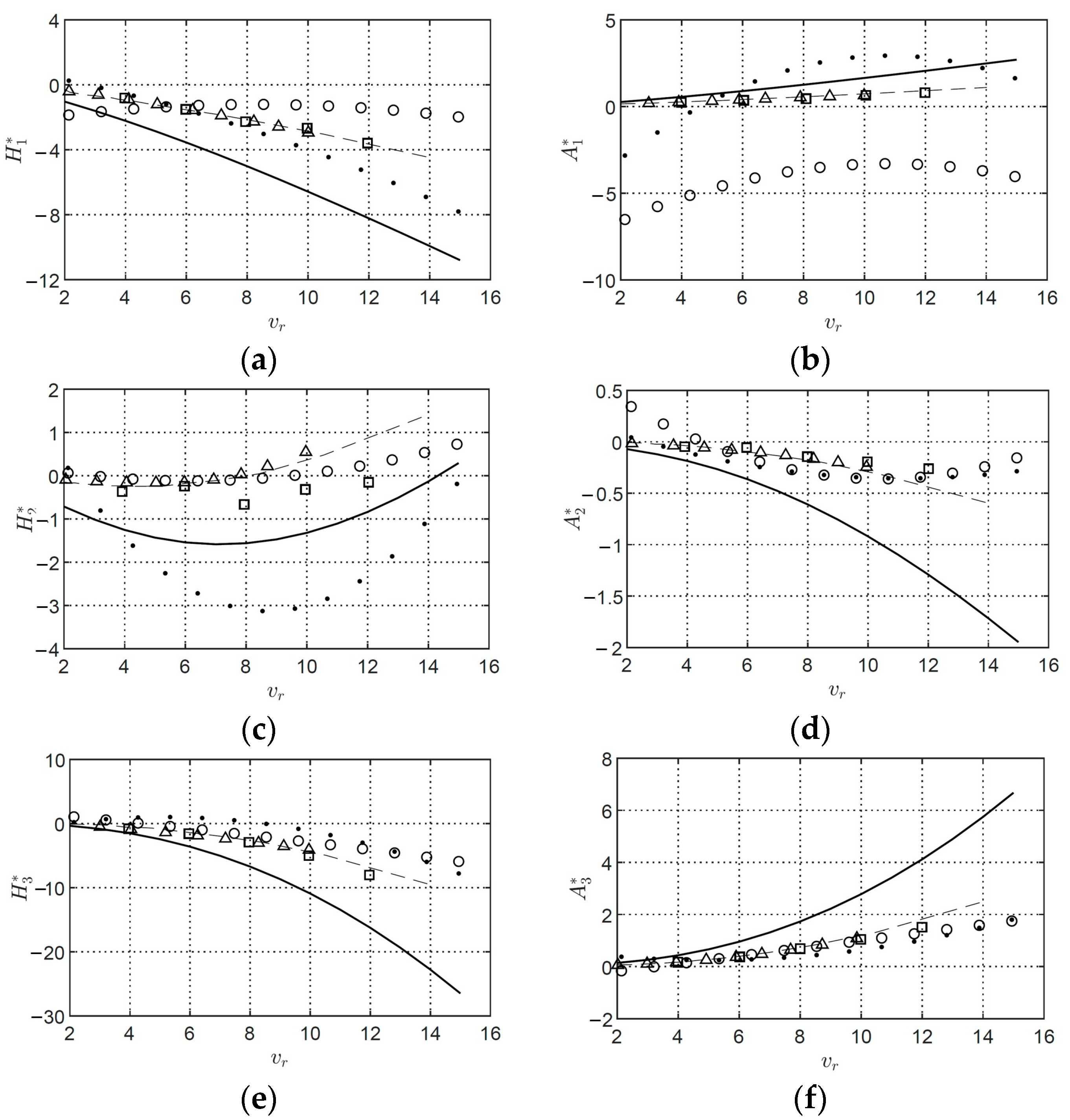
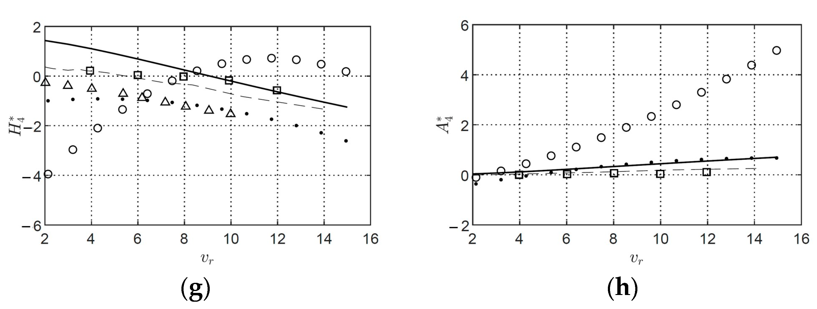
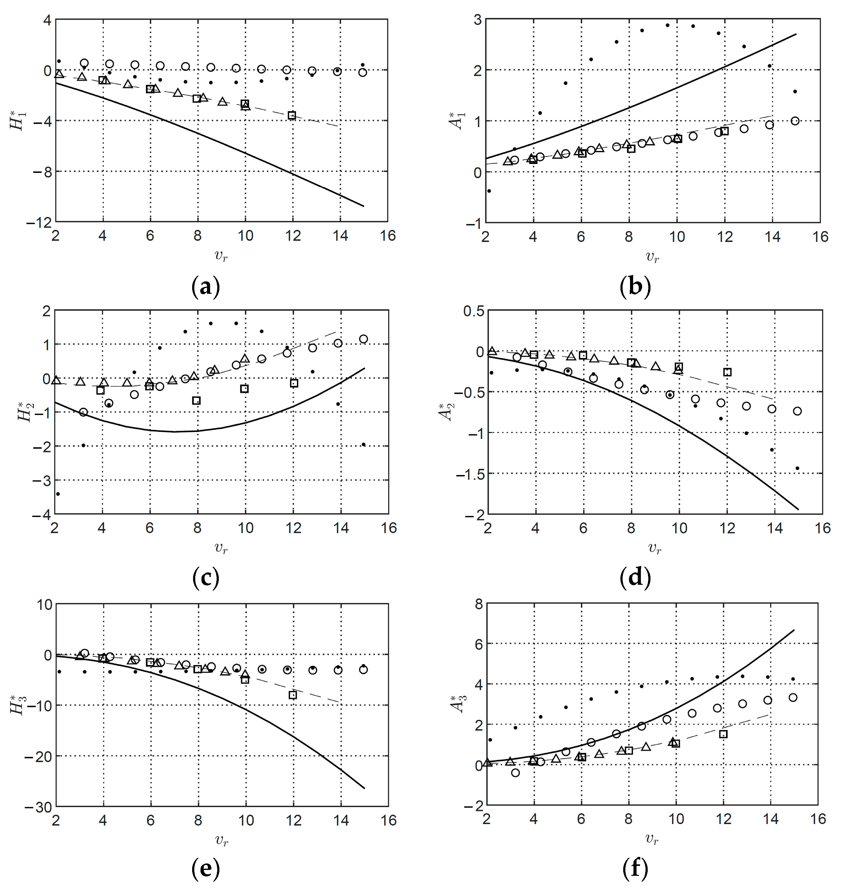
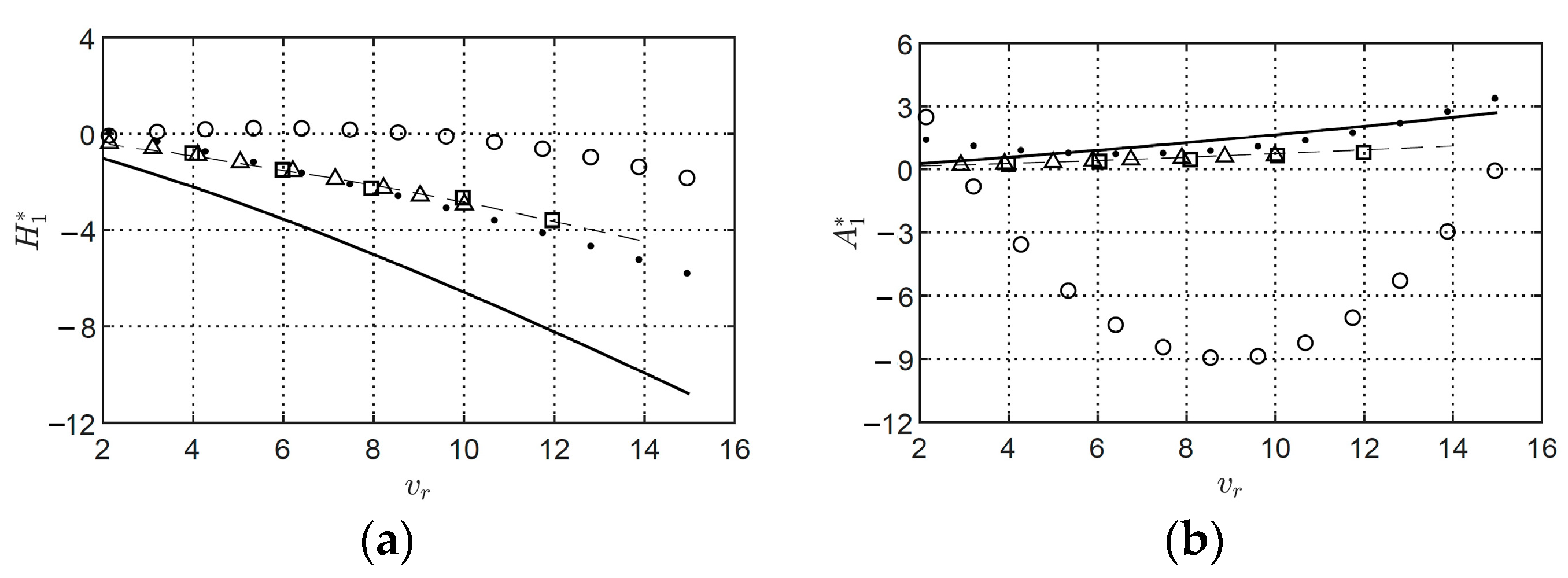
12. Validation of the Flutter Derivatives Extracted Using the MITD, ILS, and CFD Methods

The direct and cross-flutter derivatives are identified from SDOF and 2DOF tests using system identification methods. Only flutter derivatives from heave-dominant motion in Setup 1 are used because of their reasonable values. These derivatives are validated with CFD simulation results. Direct flutter derivatives, $H_1^{*}$, $H_4^{*}$, $A_2^{*}$, and $A_3^{*}$, are computed using ITD and MITD methods and show good agreement and clear patterns. Some discrepancies at high reduced wind speeds are due to noise and short signals. $H_1^{*}$ and $H_4^{*}$ are associated with heave and pitch motion, respectively, and show close agreement with the CFD results. $H_3^{*}$ and $A_4^{*}$ values from both methods are similar and agree with the theoretical and numerical values. $H_4^{*}$ values from the MITD and ILS methods deviate due to different frequency values. $H_2^{*}$ and $A_1^{*}$ are associated with coupled motion and have different values from both methods. Both methods successfully computed flutter derivatives with some uncertainties that can be reduced by additional experiments. The CFD simulation results also show good agreement with the experimental results.

13. Conclusions

This research suggests that wind tunnel tests are still reliable in investigating the aerodynamics of long-span bridges, but the design of the experimental setup is crucial to the results. In this study, Setup 1 achieved SDOF heave and pitch but suffered from a lot of damping and noise. Setup 2 reduced the damping but introduced an additional mode, affecting results. The nonlinearity of the SDOF response was due to large initial displacements. The filtration process should be carefully considered, as a wrong filter can remove important information. The system identification methods showed good results except for Logarithmic-Decrement Method, with Hilbert Transform Method being the most effective due to its capability of extracting both damping and frequency from the nonlinear response.

Direct flutter derivatives closely match the experimental results, except for $H_4^{*}$, which is difficult to identify accurately due to small frequency shifts at higher wind speeds. The HTM shows a stable decreasing trend in $H_4^{*}$. Modal frequencies and system parameters extracted using the ITD and MITD methods with Setup 1 were more reasonable than those of Setup 2, which had an additional dominant mode, causing poor-quality responses. Setup 1 can be improved with modifications without allowing unrestricted motion. The MITD parameter quality depends on the quality of the simulated signal. Separating heave and pitch components improves signal and parameter quality, with MITD converging faster than ILS in up to seven iterations versus up to eighty iterations, respectively.

The accuracy of system parameters and flutter derivatives can be improved by repeating wind tunnel tests. The flutter derivatives obtained from numerical CFD simulations showed good agreement with the flat plate results. Despite limitations, valuable results were still obtained from the noisy data. Overall, the experimental and numerical results are comparable to flat plates, which confirms the streamlined behavior of the Great Belt section from an aerodynamic perspective.

Wind tunnel tests are reliable for investigating the aerodynamics of long-span bridges, but the experimental setup is crucial. The Hilbert transform method is effective for system identification. The results confirm the streamlined behavior of the Great Belt section from an aerodynamic perspective.

The accuracy of the system parameters and flutter derivatives can be improved by repeating wind tunnel tests with multiple sensors. Techniques such as stochastic subspace identification (SSI) and enhanced frequency domain decomposition (EFDD) could also be utilized for the identification of modal parameters for more comparison options.

References

1. Ali, K.; Javed, A.; Mustafa, A.E.; Saleem, A. Blast-Loading Effects on Structural Redundancy of Long-Span Suspension Bridge Using a Simplified Approach. Pract. Period. Struct. Des. Constr. 2022, 27, 04022024. [Google Scholar] [CrossRef]
2. Ge, Y.J.; Xiang, H.F. Computational models and methods for aerodynamic flutter of long-span bridges. J. Wind. Eng. Ind. Aerodyn. 2008, 96, 1912–1924. [Google Scholar] [CrossRef]
3. Hameed, A.; Rasool, A.M.; Ibrahim, Y.E.; Afzal, M.F.U.D.; Qazi, A.U.; Hameed, I. Utilization of Fly Ash as a Viscosity-Modifying Agent to Produce Cost-Effective, Self-Compacting Concrete: A Sustainable Solution. Sustainability 2022, 14, 11559. [Google Scholar] [CrossRef]
4. Su, Y.; Di, J.; Li, S.; Jian, B.; Liu, J. Buffeting Response Prediction of Long-Span Bridges Based on Different Wind Tunnel Test Techniques. Appl. Sci. 2022, 12, 3171. [Google Scholar] [CrossRef]
5. Afzal, M.F.U.D.; Matsumoto, Y.; Nohmi, H.; Sakai, S.; Su, D.; Nagayama, T. Comparison of Radar Based Displacement Measurement Systems with Conventional Systems in Vibration Measurements at a Cable Stayed Bridge, Osaka, Japan, August 2016. Available online: https://www.researchgate.net/publication/307932143 (accessed on 17 March 2023).
6. Yu, H.; Xu, F.; Ma, C.; Zhou, A.; Zhang, M. Experimental research on the aerodynamic responses of a long-span pipeline suspension bridge. Eng. Struct. 2021, 245, 112856. [Google Scholar] [CrossRef]
7. Javed, A.; Krishna, C.; Ali, K.; Afzal, M.F.U.D.; Mehrabi, A.; Meguro, K. Micro-Scale Experimental Approach for the Seismic Performance Evaluation of RC Frames with Improper Lap Splices. Infrastructures 2023, 8, 56. [Google Scholar] [CrossRef]
8. Hua, X.; Wang, C.; Li, S.; Chen, Z. Experimental investigation of wind-induced vibrations of main cables for suspension bridges in construction phases. J. Fluids Struct. 2020, 93, 102846. [Google Scholar] [CrossRef]
9. Ma, C.M.; Duan, Q.S.; Liao, H.L. Experimental investigation on aerodynamic behavior of a long span cable-stayed bridge under construction. KSCE J. Civ. Eng. 2018, 22, 2492–2501. [Google Scholar] [CrossRef]
10. Cardenas, C.S.; Mantawy, I.M.; Azizinamini, A. Repair of Timber Piles Using Ultra-High-Performance Concrete: Investigation of Load Transfer and Load-Carrying Capacity. Transp. Res. Rec. J. Transp. Res. Board 2022, 036119812211211. [Google Scholar] [CrossRef]
11. Ashraf, S.; Ali, M.; Shrestha, S.; Hafeez, M.A.; Moiz, A.; Sheikh, Z.A. Impacts of climate and land-use change on groundwater recharge in the semi-arid lower Ravi River basin, Pakistan. Groundw. Sustain. Dev. 2022, 17, 100743. [Google Scholar] [CrossRef]
12. Arvan, P.A.; Arockiasamy, M. Energy-Based Approach: Analysis of a Vertically Loaded Pile in Multi-Layered Non-Linear Soil Strata. Geotechnics 2022, 2, 549–569. [Google Scholar] [CrossRef]
13. Zhang, H.; Liu, L.; Dong, M.; Sun, H. Analysis of wind-induced vibration of fluid-structure interaction system for isolated aqueduct bridge. Eng. Struct. 2013, 46, 28–37. [Google Scholar] [CrossRef]
14. Javed, A.; Sadeghnejad, A.; Rehmat, S.; Yakel, A.; Azizinamini, A. Magnetic Flux Leakage (MFL) Method for Damage Detection in Internal Post-Tensioning Tendons; Florida International University: Miami, FL, USA, 2021. [Google Scholar] [CrossRef]
15. Zhao, G.; Wang, Z.; Zhu, S.; Hao, J.; Wang, J. Experimental Study of Mitigation of Wind-Induced Vibration in Asymmetric Cable-Stayed Bridge Using Sharp Wind Fairings. Appl. Sci. 2022, 12, 242. [Google Scholar] [CrossRef]
16. Zhu, L.D.; Wang, M.; Wang, D.L.; Guo, Z.S.; Cao, F.C. Flutter and buffeting performances of Third Nanjing Bridge over Yangtze River under yaw wind via aeroelastic model test. J. Wind. Eng. Ind. Aerodyn. 2007, 95, 1579–1606. [Google Scholar] [CrossRef]
17. Tang, H.; Zhang, H.; Mo, W.; Li, Y. Flutter performance of box girders with different wind fairings at large angles of attack, Wind and Structures. Int. J. 2021, 32, 509–520. [Google Scholar] [CrossRef]
18. Laima, S.; Li, H.; Chen, W.; Ou, J. Effects of attachments on aerodynamic characteristics and vortex-induced vibration of twin-box girder. J. Fluids Struct. 2018, 77, 115–133. [Google Scholar] [CrossRef]
19. Tacoma Narrows Bridge (Sturdy Gertie)—HistoricBridges.org, (n.d.). Available online: https://historicbridges.org/bridges/browser/?bridgebrowser=washington/tacomanarrowsbridge/ (accessed on 6 March 2023).
20. Ge, Y.; Zhao, L.; Cao, J. Case study of vortex-induced vibration and mitigation mechanism for a long-span suspension bridge. J. Wind. Eng. Ind. Aerodyn. 2022, 220, 104866. [Google Scholar] [CrossRef]
21. Alamdari, M.M.; Rakotoarivelo, T.; Khoa, N.L.D. A spectral-based clustering for structural health monitoring of the Sydney Harbour Bridge. Mech. Syst. Signal Process. 2017, 87, 384–400. [Google Scholar] [CrossRef]
22. Mustafa, A.E.; Javed, A.; Ali, K. Safety Assessment of Cables of Suspension Bridge under Blast Load. Struct. Congr. 2022 2022, 2022, 79–93. [Google Scholar] [CrossRef]
23. Javed, A.; Mantawy, I.M.; Azizinamini, A. 3D-Printing of Ultra-High-Performance Concrete for Robotic Bridge Construction. SAGE J. 2021, 2675, 307–319. [Google Scholar] [CrossRef]
24. Fei, H.; Deng, Z.; Dan, D. Vertical Vibrations of Suspension Bridges: A Review and a New Method. Arch. Comput. Methods Eng. 2021, 28, 1591–1610. [Google Scholar] [CrossRef]
25. Larsen, A.; Larose, G.L. Dynamic wind effects on suspension and cable-stayed bridges. J. Sound Vib. 2015, 334, 2–28. [Google Scholar] [CrossRef]
26. Weber, F.; Maślanka, M. Frequency and damping adaptation of a TMD with controlled MR damper. Smart Mater. Struct. 2012, 21, 055011. [Google Scholar] [CrossRef]
27. Fujino, Y.; Siringoringo, D. Vibration mechanisms and controls of long-span bridges: A review. Struct. Eng. Int. 2013, 23, 248–268. [Google Scholar] [CrossRef]
28. Battista, R.C.; Pfeil, L.S. Reduction of vortex-induced oscillations of Rio–Niterói bridge by dynamic control devices. J. Wind. Eng. Ind. Aerodyn. 2000, 84, 273–288. [Google Scholar] [CrossRef]
29. Larsen, A.; Danish Maritime Institute. Aerodynamics of Large Bridges: Proceedings of the First International Symposium on Aerodynamics of Large Bridges; Routledge: Copenhagen, Denmark, 1992. [Google Scholar]
30. Theodorsen, T. General Theory of Aerodynamic Instability and the Mechanism of Flutter. 1949; NASA Technical Reports Server (NTRS). Available online: https://ntrs.nasa.gov/citations/19930090935 (accessed on 6 March 2023).
31. Assessment of Numerical Prediction Models for Aeroelastic Instabilities of Bridges. Available online: https://www.researchgate.net/publication/325165262_Assessment_of_Numerical_Prediction_Models_for_Aeroelastic_Instabilities_of_Bridges (accessed on 6 March 2023).
32. Chowdhury, A.G.; Sarkar, P.P. Identification of Eighteen Flutter Derivatives of an Airfoil and a Bridge Deck. Wind. Struct. 2004, 7, 187–202. [Google Scholar] [CrossRef]
33. Chowdhury, A.G.; Sarkar, P.P. A new technique for identification of eighteen flutter derivatives using a three-degree-of-freedom section model. Eng. Struct. 2003, 25, 1763–1772. [Google Scholar] [CrossRef]
34. Sarkar, B.P.P.; Member, A.; Jones, N.P.; Scanlan, R.H.; Member, H. Identification of aeroelastic parameters of flexible bridges. J. Eng. Mech. 1994, 120, 1718–1742. [Google Scholar] [CrossRef]
35. Kavrakov, I.; Morgenthal, G. A synergistic study of a CFD and semi-analytical models for aeroelastic analysis of bridges in turbulent wind conditions. J. Fluids Struct. 2018, 82, 59–85. [Google Scholar] [CrossRef] [Green Version]
36. Cassaro, M.; Cestino, E.; Frulla, G.; Marzocca, P.; Pertile, M. Experimental Determi-nation of Aeroelastic Derivatives for a Small-Scale Bridge Deck. Int. J. Mech. 2018, 12, 67–68. Available online: https://hal.science/hal-02315065 (accessed on 6 March 2023).
37. Larsen, A. Aerodynamic aspects of the final design of the 1624 m suspension bridge across the Great Belt. J. Wind. Eng. Ind. Aerodyn. 1993, 48, 261–285. [Google Scholar] [CrossRef]
38. Frandsen, J.B. Simultaneous Pressures and Accelerations Measured Full-Scale on the Great Belt East Suspension Bridge. J. Wind. Eng. Ind. Aerodyn. 2001, 89, 95–129. [Google Scholar] [CrossRef]
39. Bauhaus-Universität Weimar: Research Equipment. Available online: https://www.uni-weimar.de/en/civil-engineering/chairs/modelling-and-simulation-of-structures/research/research-equipment/ (accessed on 6 March 2023).
40. Yang, C.; Xia, Y. A novel two-step strategy of non-probabilistic multi-objective optimization for load-dependent sensor placement with interval uncertainties. Mech. Syst. Signal Process. 2022, 176, 109173. [Google Scholar] [CrossRef]
41. Yang, C.; Ouyang, H. A novel load-dependent sensor placement method for model updating based on time-dependent reliability optimization considering multi-source uncertainties. Mech. Syst. Signal Process. 2022, 165, 108386. [Google Scholar] [CrossRef]
42. Larsen, A.; Walther, J.H. Discrete vortex simulation of flow around five generic bridge deck sections. J. Wind. Eng. Ind. Aerodyn. 1998, 77, 591–602. [Google Scholar] [CrossRef]
Figure 1. Definition of degrees-of-freedom (heave h and pitch) and aeroelastic forces (lift, FL, and moment, M) for flutter analysis of flat plate [31].
Applsci 13 04672 g001
Figure 2. Typical decaying response, where x ^ is the maximum amplitude, and x n and x n + j are successive peak amplitudes.
Applsci 13 04672 g002
Figure 3. Flowchart of the iterative squares approach (ILS) algorithm [33].
Applsci 13 04672 g003
Figure 4. Flowchart of the modified Ibrahim time domain method (MITD) algorithm.
Applsci 13 04672 g004
Figure 5. General arrangement of the Great Belt Bridge: deck cross-section (top) and bridge elevation (bottom) [37,38].
Applsci 13 04672 g005
Figure 6. (a) Great Belt Bridge deck cross-section; (b) skeleton of the bridge deck model.
Applsci 13 04672 g006
Figure 7. Three-dimensional model of the wind tunnel facility at Bauhaus-Universität Weimar [39].
Applsci 13 04672 g007
Figure 8. Three-dimensional model of test setup arrangement.
Applsci 13 04672 g008
Figure 9. Possible-degree-of-freedoms of the system, where h = vertical displacement, α = rotation, p = displacement along the wind direction (restricted), r = horizontal displacement (restricted), and ro = rocking of section model (restricted).
Applsci 13 04672 g009
Figure 10. Single-degree-of-freedom assembly: (a) torsional DOF assembly; (b) vertical DOF assembly.
Applsci 13 04672 g010
Figure 11. Two-degree-of-freedom assembly: (a) Setup 1, utilizing all components; (b) Setup 2, without bearing assemblies.
Applsci 13 04672 g011
Figure 12. Recorded response of SDOF pitch: (a) raw acceleration time history at U = 0 m/s; (b) raw acceleration time history at U = 10 m/s.
Applsci 13 04672 g012
Figure 13. Filtered response of SDOF pitch response: (a) filtered acceleration time history at U = 0 m/s; (b) filtered acceleration time history at U = 10 m/s.
Applsci 13 04672 g013
Figure 14. Time history: (a) vertical at U = 0 m/s; (b) vertical at U = 10 m/s; (c) torsional at U = 0 m/s; (d) torsional at U = 10 m/s.
Applsci 13 04672 g014
Figure 15. Dominant coupled response from Setup 1: (a) vertical at U = 0 m/s; (b) vertical at U = 10 m/s; (c) torsional at U = 0 m/s; (d) torsional at U = 10 m/s.
Applsci 13 04672 g015
Figure 16. FFTs of the dominant coupled responses from Setup 1: (a) vertical response at U = 0 m/s; (b) vertical response at U = 10 m/s; (c) torsional response at U = 0 m/s; (d) torsional response at U = 10 m/s.
Applsci 13 04672 g016
Figure 17. Dominant coupled responses from Setup 2: (a) vertical response at U = 0 m/s; (b) vertical response at U = 10 m/s; (c) torsional response at U = 0 m/s; (d) torsional response at U = 10 m/s.
Applsci 13 04672 g017
Figure 18. FFTs of dominant coupled responses from Setup 2: (a) vertical response at U = 0 m/s; (b) vertical response at U = 10 m/s; (c) torsional response at U = 0 m/s; (d) torsional response at U = 10 m/s.
Applsci 13 04672 g018
Figure 19. Vertical-dominant coupled responses from Setup 1: (a) vertical displacement at U = 0 m/s; (b) vertical displacement at U = 10 m/s; (c) torsional displacement at U = 0 m/s; (d) torsional displacement at U = 10 m/s.
Applsci 13 04672 g019
Figure 20. Torsional=dominant coupled responses from Setup 1: (a) vertical displacement at U = 0 m/s; (b) vertical displacement at U = 10 m/s; (c) torsional displacement at U = 0 m/s; (d) torsional displacement at U = 10 m/s.
Applsci 13 04672 g020aApplsci 13 04672 g020b
Figure 21. Damping values: (―) Hilbert transform method, (O) polynomial fit of the exponential decay curve fitting method, (∆) polynomial fit of logarithmic decrement method. (a) Heave response; (b) pitch response.
Applsci 13 04672 g021
Figure 22. Frequency values: (―) Hilbert transform method, (O) frequency obtained through FFT of filtered acceleration response. (a) Heave response; (b) pitch response.
Applsci 13 04672 g022
Figure 23. Aerodynamics derivatives of Great Belt section: () polynomial fit of exponential decay curve, () Hilbert transform method, (●) polynomial fit of logarithmic decrement method, () wind tunnel test [42], (∆) wind tunnel test [2], (− −) water channel tests, () flat plate by Theodorsen. (a) H 1 * ; (b) H 4 * ; (c) A 2 * ; (d) A 3 * .
Applsci 13 04672 g023
Figure 24. Aerodynamics derivatives of Great Belt Section: (●) modified Ibrahim time domain method, () iterative least square method, () wind tunnel test (Larsen et al.) [42], (∆) wind tunnel test (Ge et al.) [2], (− −) water channel tests, (―) flat plate by Theodorsen. (a) H 1 * ; (b) H 4 * ; (c) A 2 * ; (d) A 3 * .
Applsci 13 04672 g024aApplsci 13 04672 g024b
Figure 25. System frequencies (heave (fh) and pitch (fα)) extracted from the MITD method at different wind speeds. (o) f α , (…) f h , (− −) f h lowpass-filtered signal FFT, (―) f α lowpass-filtered signal FFT. (a) heave-dominant, Setup 1; (b) pitch-dominant, Setup 1; (c) heave-dominant, Setup 2; (d) pitch-dominant, Setup 2.
Applsci 13 04672 g025
Figure 26. Comparison of aerodynamics derivatives from 2DOF test for Setup 1. (o) Polynomial fit from pitch using MITD method, (…) polynomial fit from heave using MITD method, (□) wind tunnel test (Larsen et al.) [42], (∆) wind tunnel test [2], (− −) water channel tests, (―) flat plate by Theodorsen. (a) H 1 * ; (b) A 1 * ; (c) H 2 * ; (d) A 2 * ; (e) H 3 * ; (f) A 3 * ; (g) H 4 * ; (h) A 4 * .
Applsci 13 04672 g026aApplsci 13 04672 g026b
Figure 27. Comparison of aerodynamics derivatives from 2DOF for Setup 2. (o) Polynomial fit from pitch using MITD method, (…) polynomial fit from heave using MITD method, (□) wind tunnel test [42], (∆) wind tunnel test [2], (− −) water channel tests, (―) flat plate by Theodorsen. (a) H 1 * ; (b) A 1 * ; (c) H 2 * ; (d) A 2 * ; (e) H 3 * ; (f) A 3 * ; (g) H 4 * ; (h) A 4 * .
Applsci 13 04672 g027aApplsci 13 04672 g027b
Figure 28. Comparison of aerodynamics derivatives from 2DOF test for Setup 1. (o) Polynomial fit from pitch using ILS method, (…) polynomial fit from heave using ILS method, (□) wind tunnel test [42], (∆) wind tunnel test [2], (− −) water channel tests, (―) flat plate by Theodorsen. (a) H 1 * ; (b) A 1 * ; (c) H 2 * ; (d) A 2 * ; (e) H 3 * ; (f) A 3 * ; (g) H 4 * ; (h) A 4 * .
Applsci 13 04672 g028aApplsci 13 04672 g028b
Figure 29. Aerodynamics derivatives from CFD simulation. (−●−) CFD forced vibration analysis, (―) flat plate by Theodorsen. (a) H 1 * ; (b) A 1 * ; (c) H 2 * ; (d) A 2 * ; (e) H 3 * ; (f) A 3 * ; (g) H 4 * ; (h) A 4 * .
Applsci 13 04672 g029