
Evaluation of the Synergies of Land Use Changes and the Quality of Ecosystem Services in the Andean Zone of Central Ecuador
 , , ,
, , ,
Abstract
:1. Introduction
2. Materials and Methods
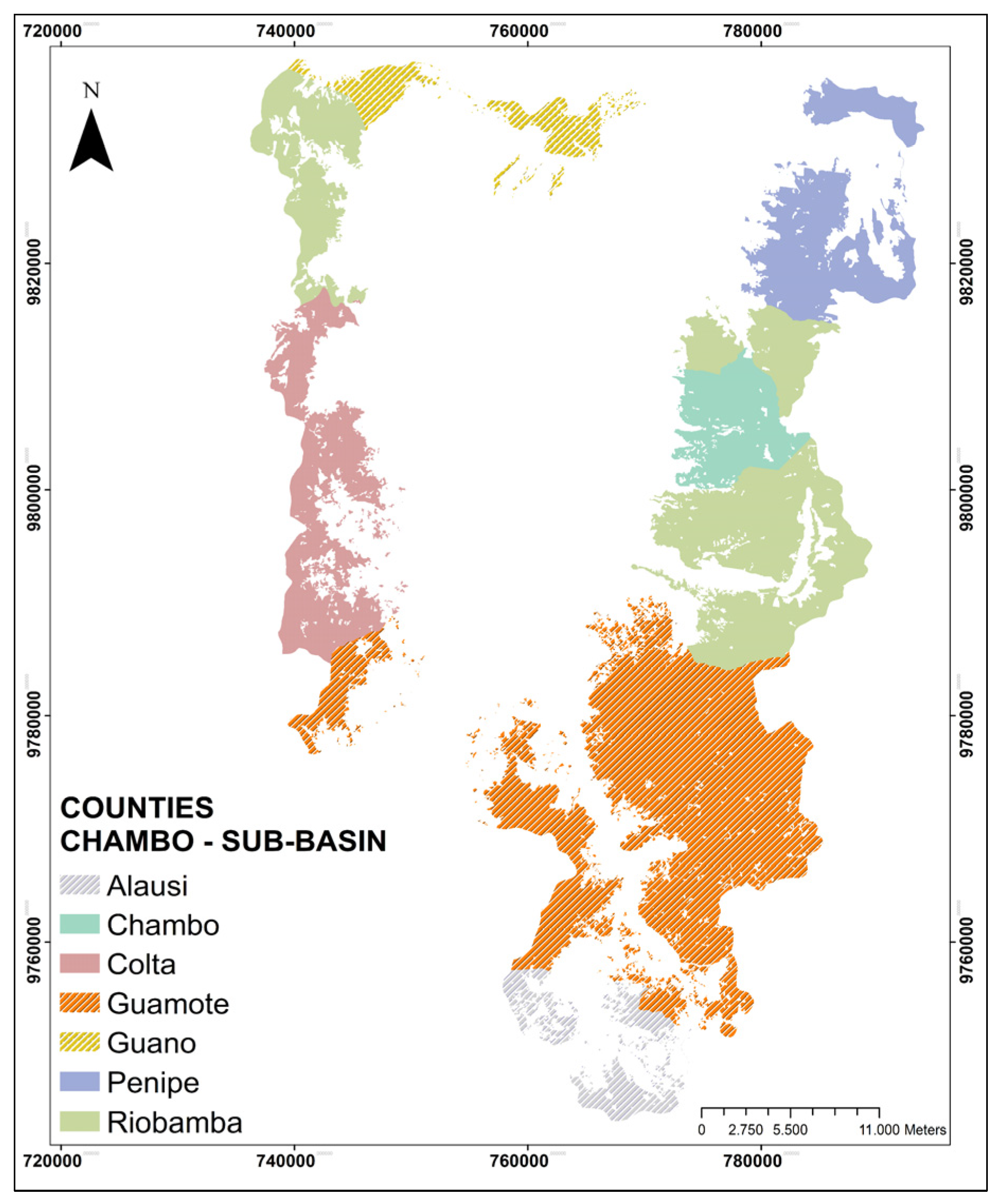
2.1. Study Area
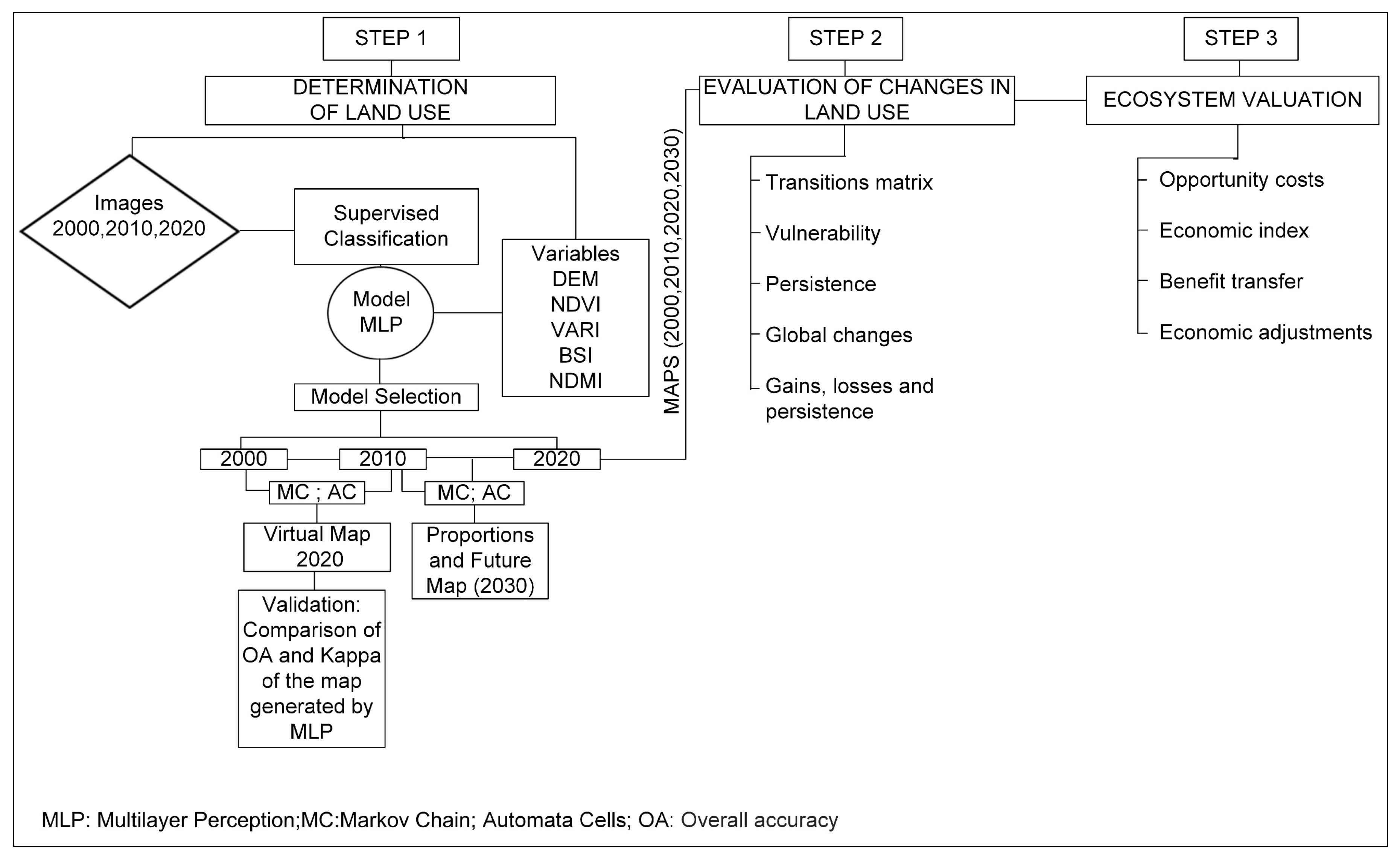
2.2. Workflow
2.3. Determination of Land Use
2.3.1. Image Processing
2.3.2. Checkpoints
2.3.3. Variables
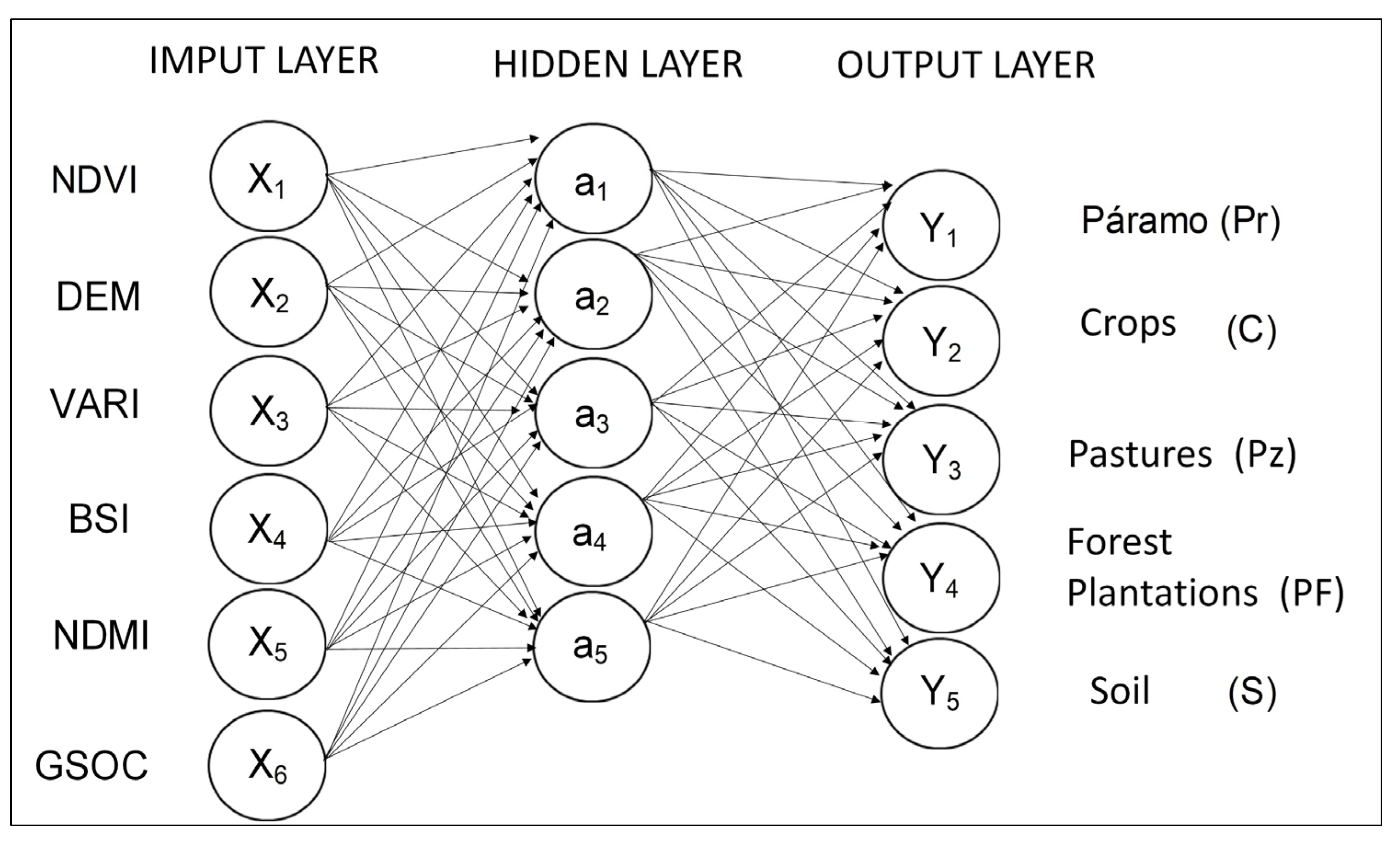
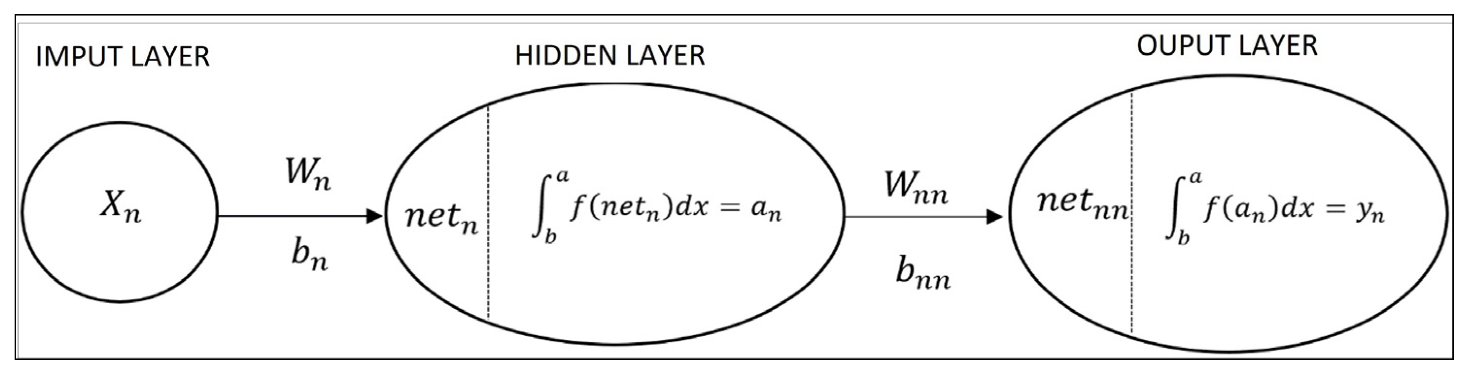
2.3.4. Land Use Classification Algorithms
2.3.5. Future Land Use Prediction Model
2.4. Evaluation of Land Use Change
2.5. Estimation of the Ecosystem Value of the Zone
3. Results
3.1. Accuracy of the Páramo Land Use Classification Algorithm and Future Land Use Prediction Model
3.2. Distribution of Land Uses in the Study Area
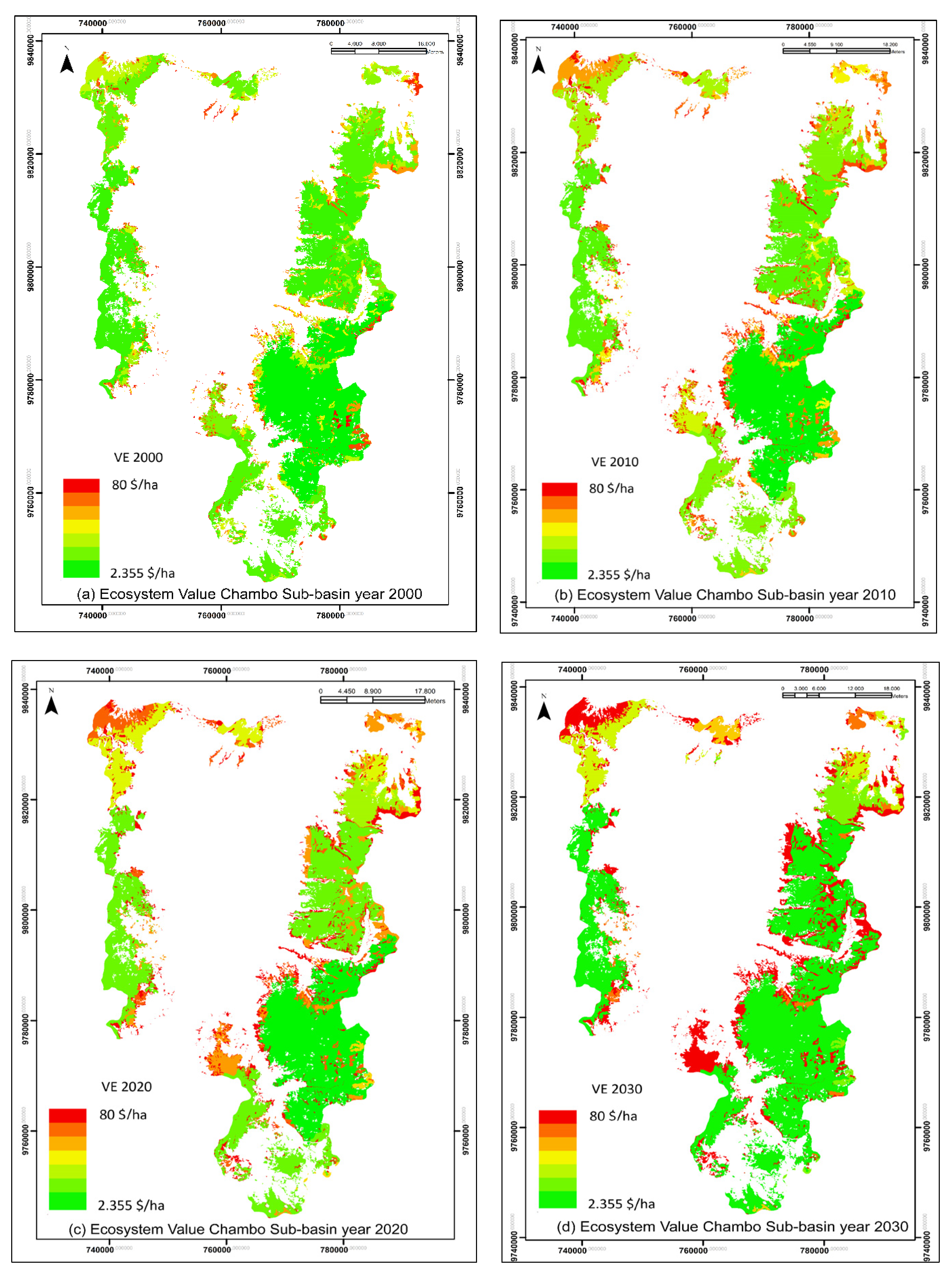
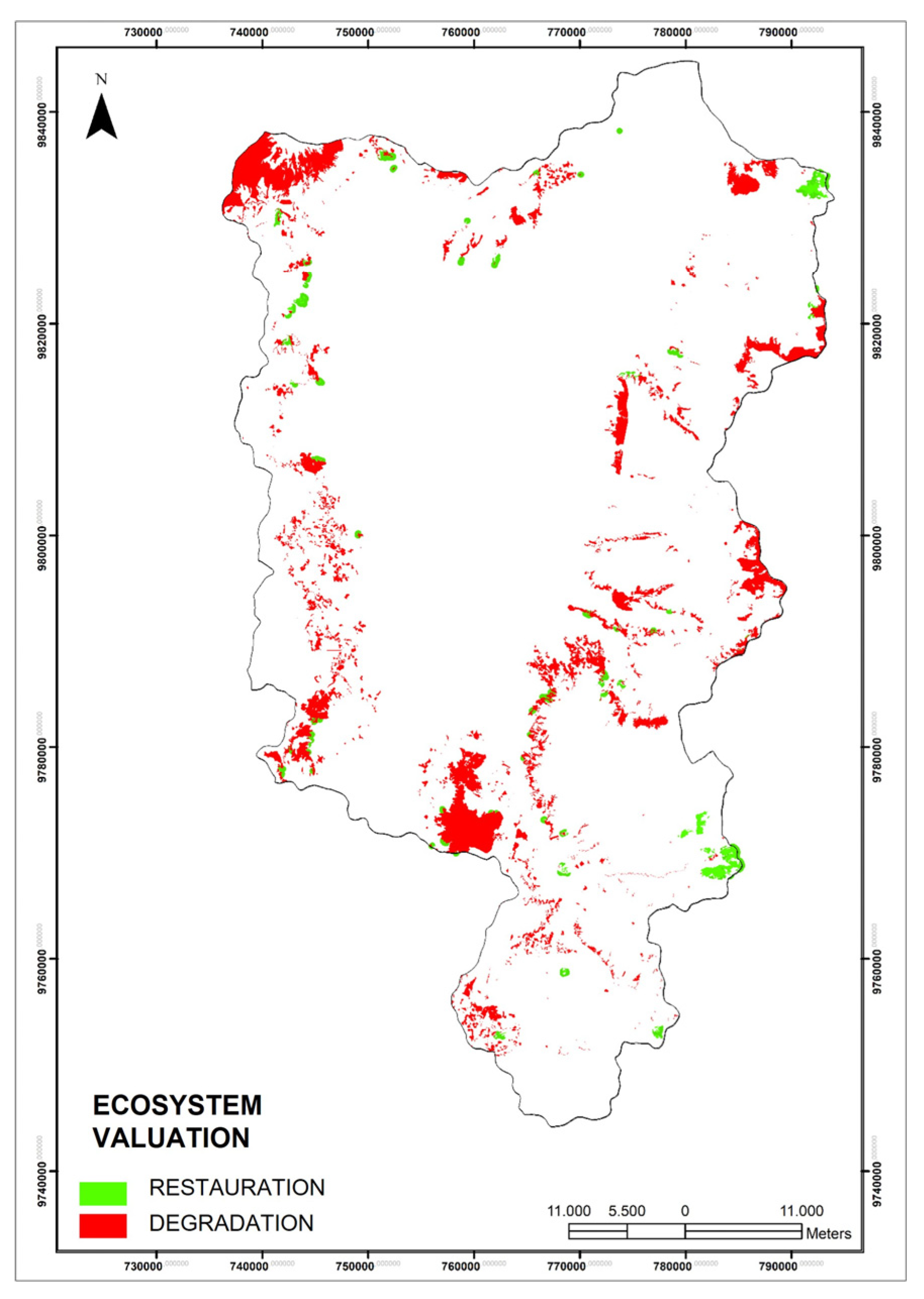
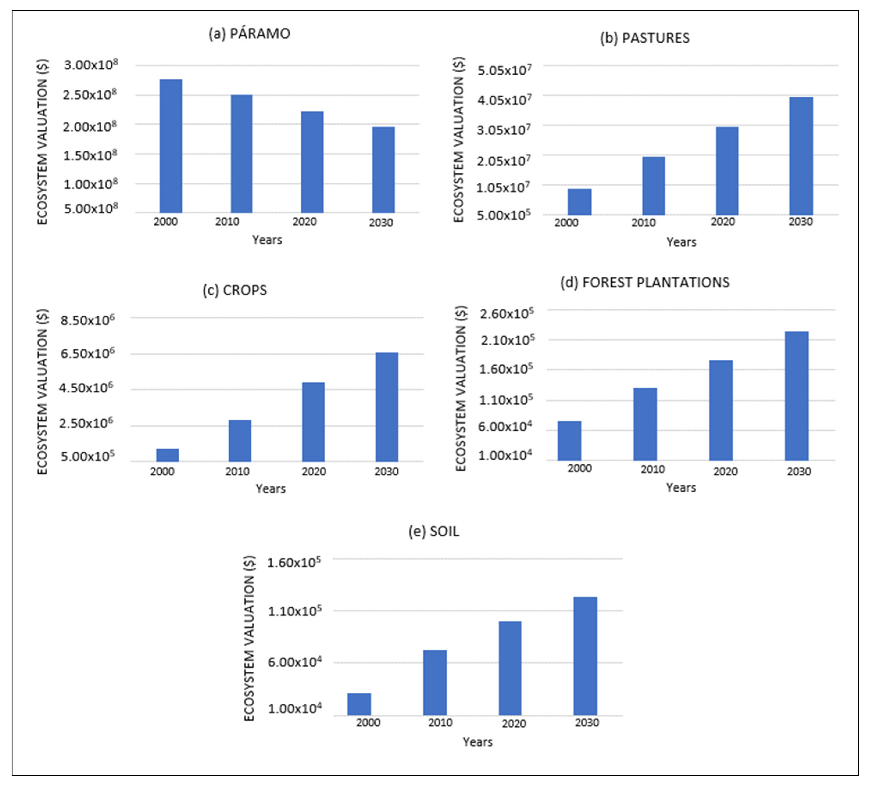
3.3. Ecosystem Valuation
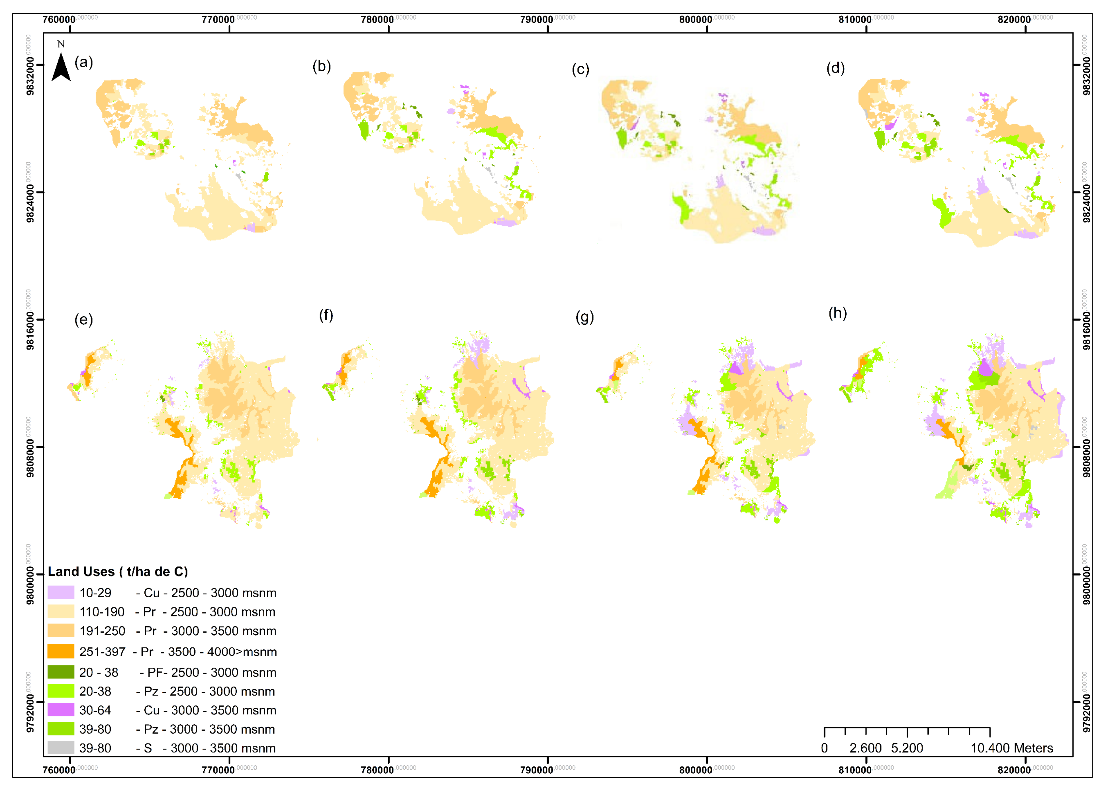
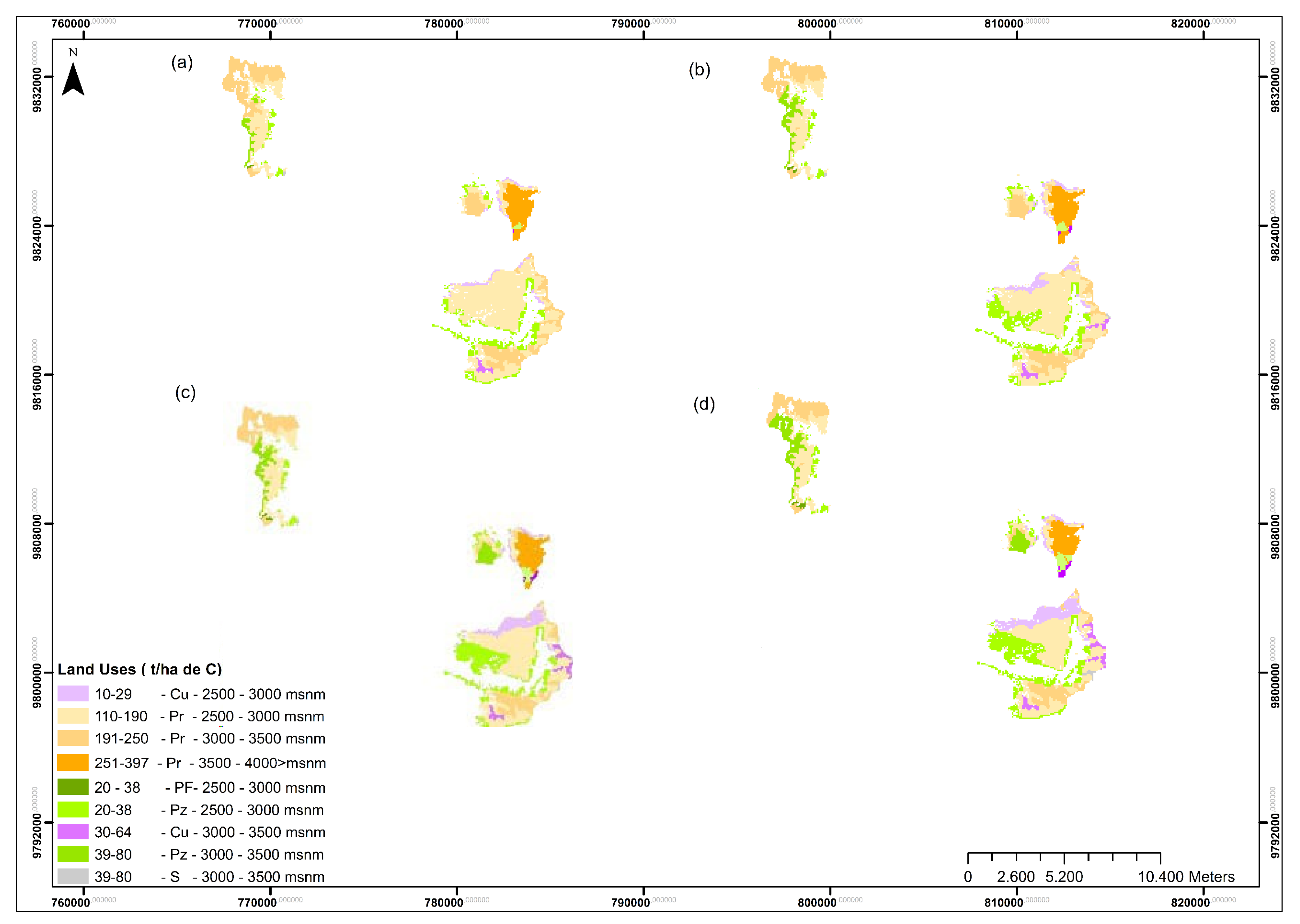
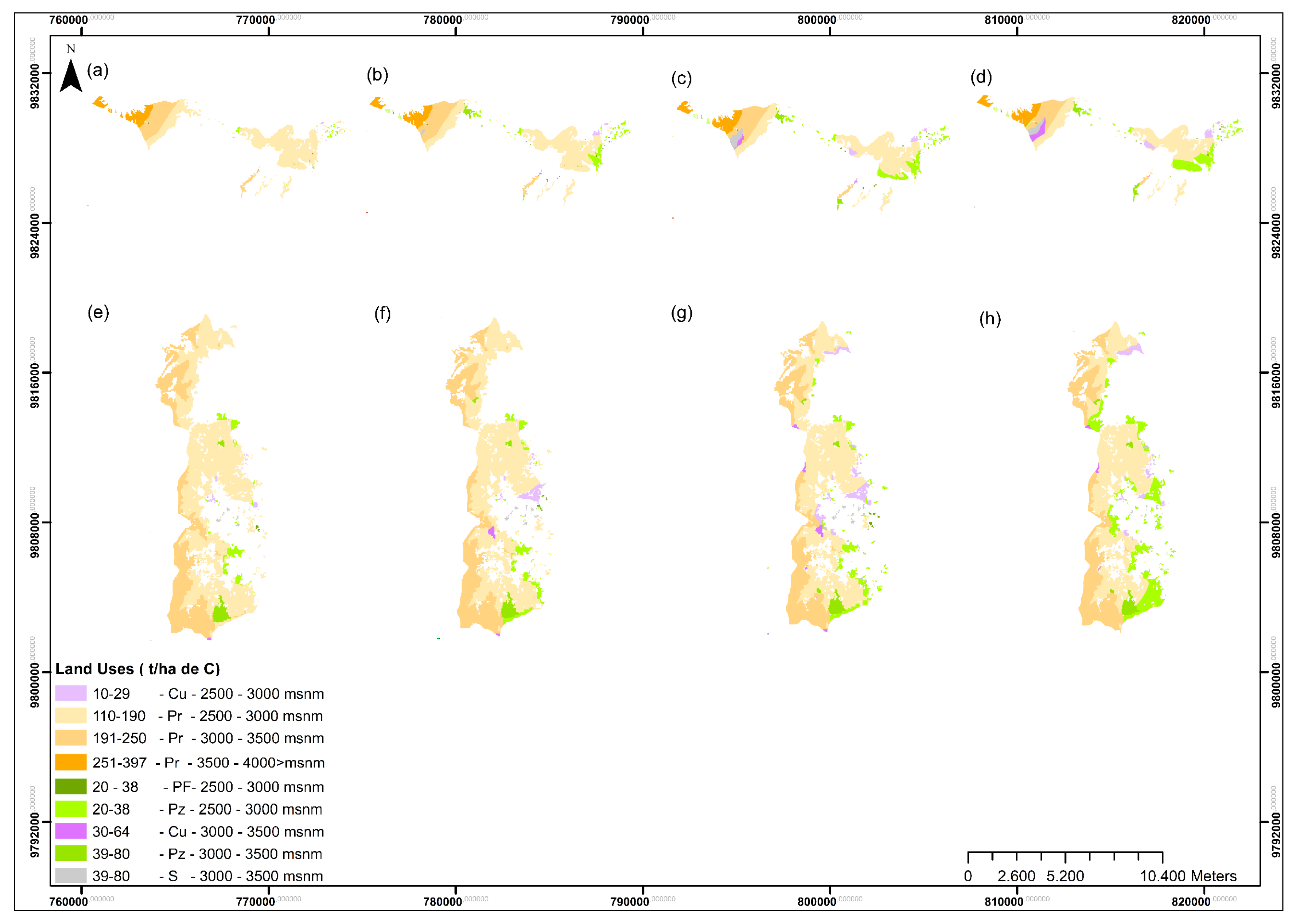
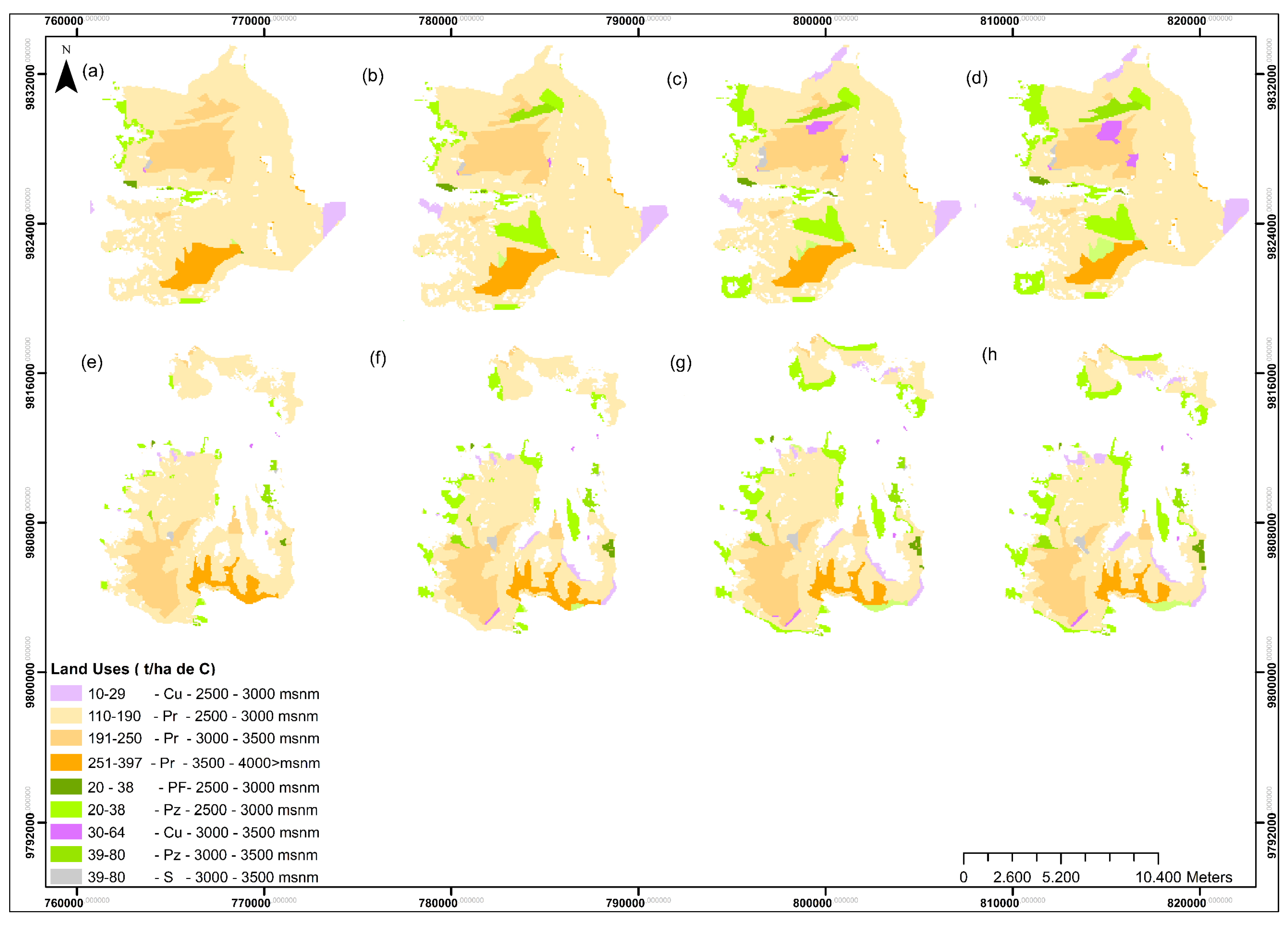
Mapping and Spatial Quantification of Ecosystem Valuation
4. Discussion
Limitations of the Study
5. Conclusions
Author Contributions
Funding
Institutional Review Board Statement
Informed Consent Statement
Data Availability Statement
Acknowledgments
Conflicts of Interest
References
- Castaño, C. Páramos and High Andean Ecosystems of Colombia in Condition of Access Point and Global Climate Tensor; IDEAM: Bogotá, Colombia, 2002. [Google Scholar]
- Hofstede, R.; Calles, J.; López, V.; Polanco, R.; Torres, F.; Ulloa, J.; Vásquez y Marcos, A. Los Páramos Andinos ¿Qué Sabemos? Estado de Conocimiento Sobre el Impacto del Cambio Climático en el Ecosistema Páramo. 2014. Available online: https://portals.iucn.org/library/node/44760 (accessed on 12 July 2023).
- García, V.; Márquez, C.; Isenhart, T.; Rodríguez, M.; Crespo, S.; Cifuentes, A. Evaluating the conservation state of the páramo ecosystem: An object-based image analysis and CART algorithm approach for central Ecuador. Heliyon 2019, 5, e02701. [Google Scholar] [CrossRef] [PubMed]
- Curatola, G.; Obermeier, W.; Gerique, A.; López, M.; Lehnert, L.; Thies, B.; Bendix, J. Land Cover Change in the Andes of Southern Ecuador—Patterns and Drivers. Remote Sens. 2015, 7, 2509–2542. [Google Scholar] [CrossRef]
- Lin, X.; Xu, M.; Xiang, H.; Ramesh, P.; Chen, W.; Ju, H. Land-use/land-cover changes and their influence on the ecosystem in chengdu city, China during the period of 1992–2018. Sustainability 2018, 10, 3580. [Google Scholar] [CrossRef]
- Pierre, H. 30 Años de Reforma Agraria y Colonización En El Ecuador: 1964–1994: DINÁMICAS ESPACIALES.; HAL: Quito, Ecuador, 2001. [Google Scholar]
- Yang, D.; Liu, W.; Tang, L.; Chen, L.; Li, X.; Xu, X. Estimation of water provision service for monsoon catchments of South China: Applicability of the InVEST model. Landsc. Urban Plan. 2019, 182, 133–143. [Google Scholar] [CrossRef]
- Suresh, S.; Lal, S. A metaheuristic framework based automated Spatial-Spectral graph for land cover classification from multispectral and hyperspectral satellite images. Infrared Phys. Technol. 2020, 105, 103–172. [Google Scholar] [CrossRef]
- Gitelson, A.; Kaufman, Y.; Stark, R.; Rundquist, D. Novel Algorithms for Remote Estimation of Vegetation Fraction. Remote Sens. Environ. 2002, 80, 76–87. [Google Scholar] [CrossRef]
- Xiao, Y.; Zhong, J.; Zhang, Q.; Xiang, X.; Huang, H. Exploring the coupling coordination and key factors between urbanization and land use efficiency in ecologically sensitive areas: A case study of the Loess Plateau, China. Sustain. Cities Soc. 2022, 86, 104148. [Google Scholar] [CrossRef]
- Delalay, M.; Tiwari, V.; Ziegler, A.D.; Gopal, V.; Passy, P. Land-use and land-cover classification using Sentinel-2 data and machine-learning algorithms, operational method and its implementation for a mountainous area of Nepal. J. Appl. Remote Sens. 2019, 13, 247–259. [Google Scholar] [CrossRef]
- Nogueira, K.; Otávio, A.; Jefersson, P.; Santos, D. Towards better exploiting convolution neural networks for remote sensing scene classification. Pattern Recognit. 2017, 61, 539–556. [Google Scholar] [CrossRef]
- Chang, Y.; Hou, X.; Li, Y.; Zhang, P.; Chen, P. Review of land Use and land cover change research progress. IOP Conf. Ser. Earth Environ. Sci. 2018, 113, 012087. [Google Scholar] [CrossRef]
- Sato, S.; Tojo, B.; Hoshi, T.; Izni, L.; Minsong, F.; Moji, K.; Kita, K. Recent Incidence of Human Malaria Caused by Plasmodium knowlesi in the Villages in Kudat Peninsula, Sabah, Malaysia: Mapping of The Infection Risk Using Remote Sensing Data. Int. J. Environ. Res. Publ. Health 2019, 16, 2954. [Google Scholar] [CrossRef] [PubMed]
- Talukdar, S.; Shahfahad, S.; Mahato, B.; Praveen, B.; Rahman, A. Dynamics of ecosystem services (ESs) in response to land use land cover (LU/LC) changes in the lower Gangetic plain of India. Ecol. Indic. 2020, 112, 106121. [Google Scholar] [CrossRef]
- Pijanowski, B.; Brown, D.; Shellito, B.; Manik, G. Using neural networks and GIS to forecast land use changes: A Land Transformation Model. Comput. Environ. Urban Syst. 2002, 26, 553–575. [Google Scholar] [CrossRef]
- Pinos, D.; Morales, O.; Duran, M. Suelos de páramo: Suelos de páramo: Análisis de percepciones de los servicios ecosistémicos y valoración económica del contenido de carbono en la sierra sureste del Ecuador. Rev. Cienc. Ambient. 2021, 55, 151–173. [Google Scholar] [CrossRef]
- Once, B.; Rivera, M.; Izurieta, C. Valoración Económica del Servicio de Provisión Hídrica de la Microcuenca del río Chimborazo. Novasinergia 2019, 2, 96–103. [Google Scholar] [CrossRef]
- Páez, A.; López, A.; Márquez, A. Evaluación Normativa, Social y Ambiental de los Páramos en Colombia; COSABE: Bogotá, Colombia, 2018. [Google Scholar]
- Rijal, S.; Techato, K.; Gyawali, S.; Stork, N.; Dangal, M.; Sinutok, S. Forest cover change and ecosystem services: A case study of community forest in mechinagar and buddhashanti landscape (MBL). Environ. Manag. 2021, 67, 963–973. [Google Scholar] [CrossRef] [PubMed]
- Ross, C.; Fildes, S.; Millington, A. Land-Use and Land-Cover Change in the Páramo of South-Central Ecuador, 1979–2014. Land 2017, 6, 46. [Google Scholar] [CrossRef]
- Amgoth, A.; Rani, H.; Jayakumar, K. Exploring LULC changes in Pakhal Lake area, Telangana, India using QGIS MOLUSCE plugin. Spat. Inf. Res. 2023, 31, 428–438. [Google Scholar] [CrossRef]
- Dinda, S.; Chatterjee, B.; Ghosh, S. Modelling the future vulnerability of urban green space for priority-based management and green prosperity strategy planning in Kolkata, India: A PSR-based analysis using AHP-FCE and ANN-Markov model. Geocarto Int. 2022, 37, 6551–6578. [Google Scholar] [CrossRef]
- Isabona, J.; Imoize, A.; Ojo, S.; Karunwi, O.; Kim, Y.; Lee, C.; Li, C. Development of a multilayer perceptron neural network for optimal predictive modeling in urban microcellular radio environments. Appl. Sci. 2022, 12, 5713. [Google Scholar] [CrossRef]
- Megahed, Y.; Cabral, P.; Silva, J.; Caetano, M. Land cover mapping analysis and urban growth modelling using remote sensing techniques in Greater Cairo Region—Egypt. ISPRS Int. J. Geo-Inf. 2015, 4, 1750–1769. [Google Scholar] [CrossRef]
- Costanza, R.; D´Arge, R.; De Groot, R.; Farber, S. The value of the world’s ecosystem services and natural capital. Nature 1987, 122, 253–260. [Google Scholar] [CrossRef]
- MAATE, Ministerio del Ambiente, Agua y Transición Ecológica del Ecuador. Sistema de Clasificación de los Ecosistemas del Ecuador Continental: SUBSECRETARÍA DE PATRIMONIO NATURAL; HAL: Quito, Ecuador, 2012. [Google Scholar]
- Quantum GIS (QGIS). Available online: https://qgis.org/es/site/forusers/download.html (accessed on 10 April 2023).
- IGM, Geoportal. 2016. Available online: https://www.geoportaligm.gob.ec/portal/ (accessed on 16 June 2023).
- Bronstert, A.; Niehoff, D.; Bürger, G. Effects of climate and land-use change on storm runoff generation: Present knowledge and modelling capabilities. Hydrol. Process. 2002, 16, 509–529. [Google Scholar] [CrossRef]
- Hu, X.; Tao, C.; Prenzel, B. Automatic Segmentation of High-resolution Satellite Imagery by Integrating Texture, Intensity, and Color Features. Photogramm. Eng. Remote Sens. 2005, 71, 45–65. [Google Scholar] [CrossRef]
- Global Soil Organic Carbon Map (GSOCmap), Geoportal. 2019. Available online: https://data.apps.fao.org/glosis/?share=f-6756da2a-5c1d-4ac9-9b94-297d1f105e83&lang=en (accessed on 16 June 2023).
- Olivares, B.; López, M. Índice de Vegetación de Diferencia Normalizada aplicado al territorio indígena agrícola de Kashaama, Venezuela. Cuad. Investig. UNED 2019, 11, 112–121. [Google Scholar] [CrossRef]
- Pinty, B.; Gobron, N.; Widlowski, J.; Lavergne, T.; Verstraete, M. Synergy between 1-D and 3-D radiation transfer models to retrieve vegetation canopy properties from remote sensing data. J. Geophys. Res. D Atmos. 2004, 109, 21205. [Google Scholar] [CrossRef]
- Feyisa, G.; Meilby, H.; Fensholt, R.; Pround, S. Automated Water Extraction Index: A new technique for surface water mapping using Landsat imagery. Remote Sens. Environ. 2014, 140, 23–35. [Google Scholar] [CrossRef]
- Altunkaynak, A.; Nigussie, T. Monthly water demand prediction using wavelet transform, first-order differencing and linear detrending techniques based on multilayer perceptron models. Urban Water J. 2018, 15, 1–5. [Google Scholar] [CrossRef]
- TerrSet Geospatial Monitoring and Modeling Software. Available online: https://clarklabs.org/terrset/ (accessed on 10 April 2023).
- Li, F.; Zhang, X.; Lu, A.; Xu, L.; Ren, D.; You, T. Estimation of metal elements content in soil using x-ray fluorescence based on multilayer perceptron. Environ. Monit. Assess. 2022, 194, 95–115. [Google Scholar] [CrossRef]
- Ding, X.; Zhao, Z.; Yang, Q.; Ch, L.; Tian, Q.; Li, X.; Meng, F. Model prediction of depth-specific soil texture distributions with artificial neural network: A case study in Yunfu, a typical area of Udults Zone, South China. Comput. Electron. Agric. 2020, 169, 100–120. [Google Scholar] [CrossRef]
- Hamad, R.; Balzter, H.; Kolo, K. Predicting land use/land cover changes using a CA-Markov model under two diferent scenarios. Sustainability 2018, 10, 3421. [Google Scholar] [CrossRef]
- Radoux, J.; Bogaert, P. Good Practices for Object-Based Accuracy Assessment. Remote Sens. 2017, 9, 646. [Google Scholar] [CrossRef]
- Aronoff, S. Classification accuracy: A user approach. Photogramm. Eng. Remote Sens. 1982, 48, 1299–1307. [Google Scholar]
- Cohen, J. A coefficient of agreement for nominal scales. Educ. Psychol. Meas. 1960, 20, 3–8. [Google Scholar] [CrossRef]
- Schmidt, K.; Sachse, R.; Walz, A. Current role of social benefits in ecosystem service assessments. Landsc. Urban Plan. 2016, 149, 49–64. [Google Scholar] [CrossRef]
- Aburas, M.; Ho, Y.; Ramli, M.; Ash’Aari, Z. The simulation and prediction of spatio-temporal urban growth trends using cellular automata models: A review. Int. J. Appl. Earth Obs. Geoinf. 2016, 12, 380–389. [Google Scholar] [CrossRef]
- MAG, Ministerio de Agricultura y Ganadería, Sistemas de Cultivos. Producción Ganadera y Lechera; HAL: Quito, Ecuador, 2020. [Google Scholar]
- Chuncho, C.; Chuncho, G. Páramos del Ecuador, importancia y afectaciones: Una revisión. Bosques Latitud Cero. 2019, 9, 71–83. Available online: https://revistas.unl.edu.ec/index.php/bosques/article/view/686 (accessed on 3 May 2023).
- Corrales, R.; Ochoa, V. Firmas espectrales de la cobertura de la Tierra, aplicando radiometría de campo. Fase 1: Región 03 occidente de Honduras. Cienc. Espac. 2014, 7, 21–36. [Google Scholar] [CrossRef]
- Fang, Z.; Chen, J.; Liu, G.; Wang, H.; Alatalo, J.; Yang, Z. Framework of basin eco-compensation standard valuation for cross-regional water supply—A case study in northern China. J. Clean. Prod. 2021, 279, 123630. [Google Scholar] [CrossRef]
- Mueller, H.; Hamilton, D.; Doole, G.; Abell, J.; McBride, C. Economic and ecosystem costs and benefits of alternative land use and management scenarios in the Lake Rotorua, New Zealand, catchment. Global Environ. Change 2019, 54, 102–112. [Google Scholar] [CrossRef]
- Hayes, T.; Murtinho, F.; Wolff, H. An institutional analysis of Payment for Environmental Services on collectively managed lands in Ecuador. Ecol. Econ. 2015, 118, 81–89. [Google Scholar] [CrossRef]
- Celleri, R.; Buytaert, W.; Feyen, J.; Íñiguez, V.; Borja, P.; Bièvre, B. Land Use Change Impacts on the Hydrology of Wet Andean Páramo Ecosystems. In Proceedings of the Status and Perspectives of Hydrology in Small Basins, Alemania, Germany, 30 March–2 April 2009. [Google Scholar] [CrossRef]
- Roldán, M.; Latorre, S. Social valuation of ecosystemic functions of streams in Quito, Ecuador. Iberoam. J. Ecol. Econ. 2021, 34, 65–85. Available online: https://raco.cat/index.php/Revibec/article/view/389020 (accessed on 3 May 2023).
- Çorumluoğlu, O.; Vural, A. Determination of Kula Basalts (Geosite) in Turkey using Remote Sensing Techniques. Arabian J. Geosci. 2015, 8, 10105–10117. [Google Scholar] [CrossRef]


| Index | Formula | Characteristics |
|---|---|---|
| NDVI: Normalized difference vegetation index | The normalized difference vegetation index (NDVI) was used to separate the vegetation from the brightness produced by the soil and to relate photosynthetic activity and leaf structure of the plants, allowing to determine the vigorousness of the plants [33]. | |
| VARI: Visible vegetation index | The visible vegetation index (VARI) allowed to observe vegetation in the visible section of the spectrum, mitigating both illumination divergences and atmospheric factors [9]. | |
| BSI: Bare soil index | It helps to identify areas of soil without vegetation, soils with vegetation and soils with scarce vegetation [34]. | |
| NDMI: Normalized difference moisture index | The Normalized Difference Moisture Index (NDMI) contributed to the detection of moisture levels in vegetation using a combination of NIR and SWIR spectral bands. It is an indicator of water stress in crops [35]. |
| Measure | Formula | Description |
|---|---|---|
| “Producer accuracy” (PA) | It is an accuracy based on references calculated from the predictions of the coverages under study, in this case: moorland, pasture, crops, forest plantations and bare soil. Based on the predictions, a percentage of correct and incorrect cover detections is established [41]. | |
| “User accuracy” (UA) | It allows to recognize the probability that a classified category actually represents the same category in the field [42]. | |
| “Overall accuracy” (OA) | Indicates the list of all reference categories that have been successfully identified [42]. | |
| Kappa Index | Analyzes the match between the data observed in the image and the data identified in the classification [43]. | |
| Profit Degradation Persistence | Gain: (Gij) = P+j − Pjj Degradation: (Lij) = Pj+ − Pjj Persistence: P+j − Gain | It contributes to the identification of changes in terms of recovery, loss and exchanges between the categories analyzed [43]. |
| Model | Variables | Accuracy (%) |
|---|---|---|
| 1 | NDVI, DEM, VARI, SOC, BSI, and NDMI. | 81 |
| 2 | NDVI, VARI, SOC, BSI, and NDMI. | 71 |
| 3 | NDVI, DEM, VARI, and SOC. | 65 |
| 4 | NDVI, DEM, and VARI. | 58 |
| 5 | NDVI and DEM. | 50 |
| 6 | NDVI. | 49 |
| Overall Accuracy (L)% | Overall Accuracy (V)% | Kappa Coefficient (L)% | Kappa Coefficient (V)% | |
|---|---|---|---|---|
| 2000 | 81 | 79 | 81 | 79 |
| 2010 | 84 | 80 | 85 | 80 |
| 2020 | 85 | 82 | 84 | 81 |
| Real Map 2020 | Projected Map 2020 | ||
|---|---|---|---|
| Scenario 1 | Kappa (%) | 81 | 60 |
| OA (%) | 82 | 63 | |
| Scenario 2 | Kappa (%) | 81 | 68 |
| OA (%) | 82 | 72 | |
| Scenario 3 | Kappa (%) | 81 | 78 |
| OA (%) | 82 | 80 |
| CANTONS | COVERAGE | 2000 (%) | 2010 (%) | 2020 (%) | 2030 (%) |
|---|---|---|---|---|---|
| Alausi | Pr | 2.8 | 2.5 | 2.0 | 1.7 |
| C | 0.0 | 0.1 | 0.3 | 1.7 | |
| Pz | 0.1 | 0.3 | 0.5 | 0.7 | |
| PF | 0.0 | 0.1 | 0.1 | 0.1 | |
| S | 0.0 | 0.0 | 0.0 | 0.1 | |
| Chambo | Pr | 5.8 | 5.0 | 4.3 | 3.7 |
| C | 0.1 | 0.3 | 0.5 | 0.6 | |
| Pz | 0.3 | 0.9 | 1.3 | 1.7 | |
| PF | 0.0 | 0.1 | 0.1 | 0.1 | |
| S | 0.0 | 0.0 | 0.1 | 0.1 | |
| Colta | Pr | 9.3 | 8.1 | 7.2 | 6.0 |
| C | 0.1 | 0.5 | 0.7 | 0.9 | |
| Pz | 0.2 | 0.9 | 1.6 | 1.2 | |
| PF | 0.0 | 0.0 | 0.1 | 0.1 | |
| S | 0.1 | 0.1 | 0.2 | 0.2 | |
| Guamote | Pr | 25.8 | 23.7 | 22.1 | 19.0 |
| C | 0.3 | 0.7 | 1.3 | 1.7 | |
| Pz | 1.5 | 3.0 | 4.0 | 6.0 | |
| PF | 0.1 | 0.1 | 0.2 | 0.2 | |
| S | 0.1 | 0.2 | 0.3 | 0.3 | |
| Guano | Pr | 3.3 | 2.6 | 2.2 | 2.0 |
| C | 0.1 | 0.2 | 0.3 | 0.5 | |
| Pz | 0.2 | 0.7 | 0.9 | 2.1 | |
| PF | 0.0 | 0.0 | 0.0 | 0.1 | |
| S | 0.0 | 0.0 | 0.1 | 0.2 | |
| Penipe | Pr | 7.3 | 6.1 | 5.2 | 3.0 |
| C | 0.1 | 0.1 | 0.1 | 0.1 | |
| Pz | 0.3 | 1.1 | 1.8 | 2.0 | |
| PF | 0.1 | 0.1 | 0.1 | 0.1 | |
| S | 0.1 | 0.3 | 0.6 | 1.0 | |
| Riobamba | Pr | 37.9 | 34.9 | 30.7 | 28.0 |
| C | 0.9 | 1.4 | 2.6 | 4.4 | |
| Pz | 3.0 | 5.1 | 7.9 | 9.5 | |
| PF | 0.2 | 0.3 | 0.4 | 0.3 | |
| S | 0.1 | 0.3 | 0.5 | 0.6 | |
| 100 | 100 | 100 | 100 |
| Land Uses | 2000 | 2000–2010 | 2010 | ||
|---|---|---|---|---|---|
| % | Persistence % | Gain% | Loss % | % | |
| Pr | 92.1 | 79.5 | 3.5 | 12.6 | 83.0 |
| C | 1.6 | 0.6 | 3.0 | 1.0 | 3.6 |
| Pz | 5.6 | 5.0 | 7.0 | 0.6 | 12.0 |
| PF | 0.4 | 0.1 | 0.6 | 0.3 | 0.7 |
| S | 0.3 | 0.1 | 0.6 | 0.3 | 0.7 |
| 100 | 100 | ||||
| Land Uses | 2010 | 2010–2020 | 2020 | ||
|---|---|---|---|---|---|
| % | Persistence % | Gain % | Loss % | % | |
| Pr | 83.0 | 63.9 | 10.1 | 19.1 | 74.0 |
| C | 3.6 | 1.0 | 5.3 | 2.6 | 6.3 |
| Gr | 12.0 | 7.0 | 10.8 | 5.0 | 17.9 |
| PF | 0.7 | 0.2 | 0.7 | 0.5 | 0.9 |
| S | 0.7 | 0.4 | 0.6 | 0.3 | 1.0 |
| 100 | 100 | ||||
| Land Uses | 2020 | 2020–2030 | 2030 | ||
|---|---|---|---|---|---|
| % | Persistence % | Gain % | Loss % | % | |
| Pr | 74.0 | 50.0 | 13.6 | 24.0 | 63.6 |
| C | 6.3 | 3.2 | 7.8 | 3.1 | 11.0 |
| Pz | 17.9 | 10.3 | 13.0 | 7.6 | 23.3 |
| PF | 0.9 | 0.2 | 0.9 | 0.8 | 1.0 |
| S | 1.0 | 0.4 | 0.8 | 0.6 | 1.2 |
| 100 | 100 | ||||
| Ecosystem Valuation—Opportunity Costs | ||
|---|---|---|
| Año | C ($/ha) | Pz ($/ha) |
| 2000 | 550 | 1000 |
| 2010 | 608 | 1313 |
| 2020 | 629 | 1370 |
| 2030 | 738 | 1401 |
| Ecosystem Valuation—Profit Transfer | ||
|---|---|---|
| Pr ($/ha) | PF ($/ha) | S ($/ha) |
| 2355 | 160 | 81 |
Disclaimer/Publisher’s Note: The statements, opinions and data contained in all publications are solely those of the individual author(s) and contributor(s) and not of MDPI and/or the editor(s). MDPI and/or the editor(s) disclaim responsibility for any injury to people or property resulting from any ideas, methods, instructions or products referred to in the content. |
© 2024 by the authors. Licensee MDPI, Basel, Switzerland. This article is an open access article distributed under the terms and conditions of the Creative Commons Attribution (CC BY) license (https://creativecommons.org/licenses/by/4.0/).
Share and Cite
Pazmiño, Y.C.; Felipe, J.J.d.; Vallbé, M.; Cargua, F.; Pazmiño, Y. Evaluation of the Synergies of Land Use Changes and the Quality of Ecosystem Services in the Andean Zone of Central Ecuador. Appl. Sci. 2024, 14, 498. https://doi.org/10.3390/app14020498
Pazmiño YC, Felipe JJd, Vallbé M, Cargua F, Pazmiño Y. Evaluation of the Synergies of Land Use Changes and the Quality of Ecosystem Services in the Andean Zone of Central Ecuador. Applied Sciences. 2024; 14(2):498. https://doi.org/10.3390/app14020498
Chicago/Turabian StylePazmiño, Yadira Carmen, José Juan de Felipe, Marc Vallbé, Franklin Cargua, and Yomara Pazmiño. 2024. "Evaluation of the Synergies of Land Use Changes and the Quality of Ecosystem Services in the Andean Zone of Central Ecuador" Applied Sciences 14, no. 2: 498. https://doi.org/10.3390/app14020498