
Numerical Equivalent Acoustic Material for Air-Filled Porous Absorption Simulations in Finite Different Time Domain Methods: Design and Comparison

Abstract
:1. Introduction
2. Materials and Methods
2.1. NEAM Model
2.2. NEAM Model Coefficients
2.3. FDTD Method
2.4. FDTD Setup
2.5. Experimental Setup
3. Results
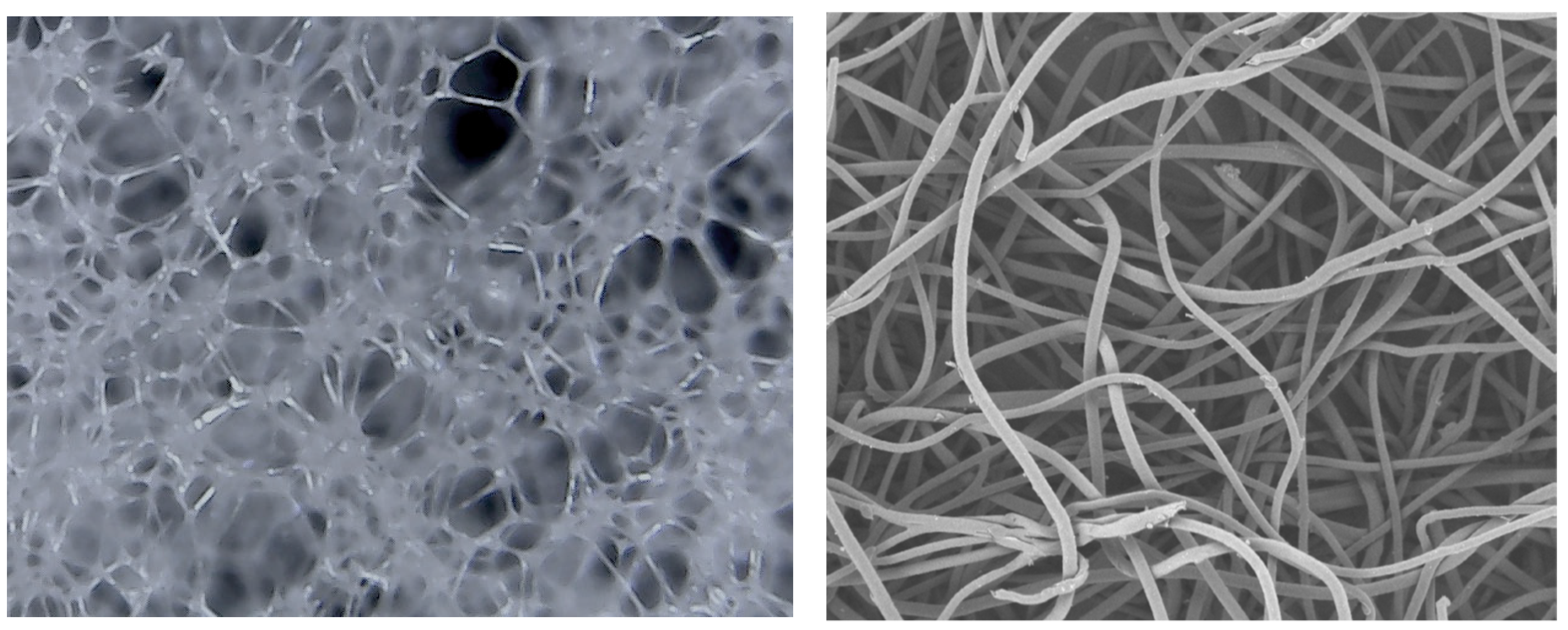
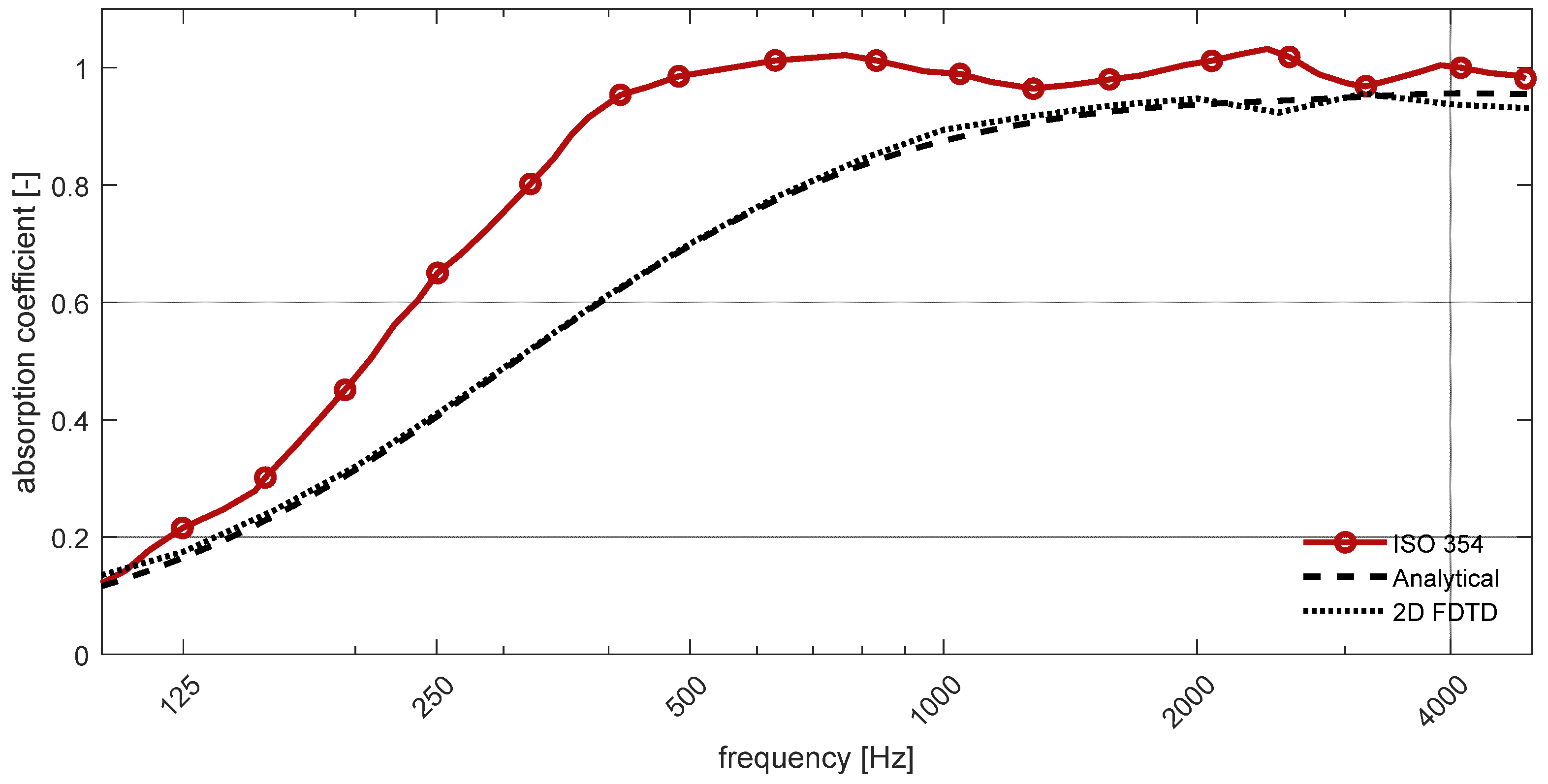
3.1. Porous Melamine Foam
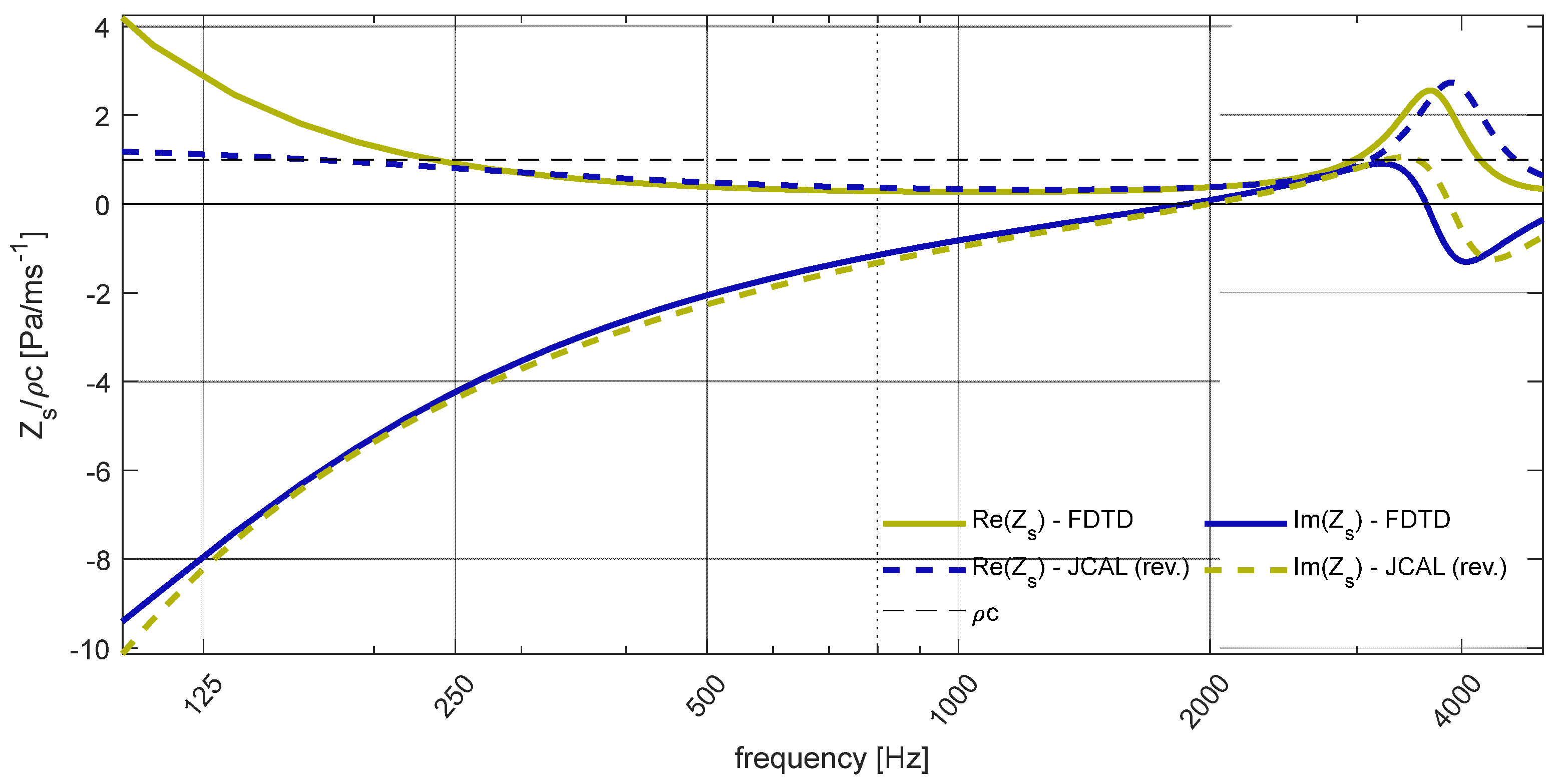
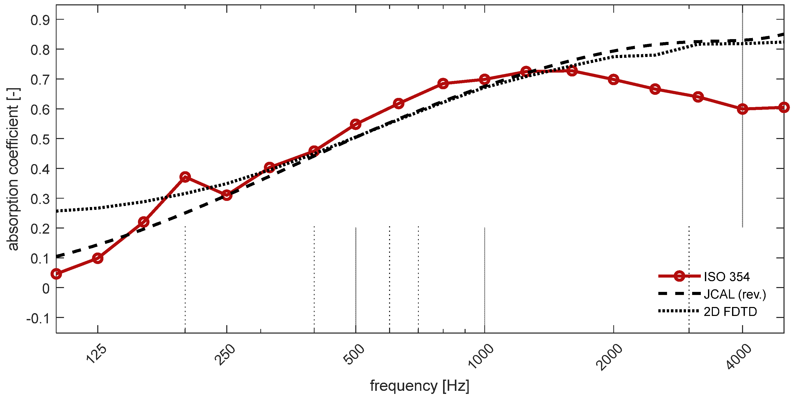
3.2. PET Fiber Sheet
3.3. NEAM Use to Extract Physical Parameters
3.4. Algorithm Performance
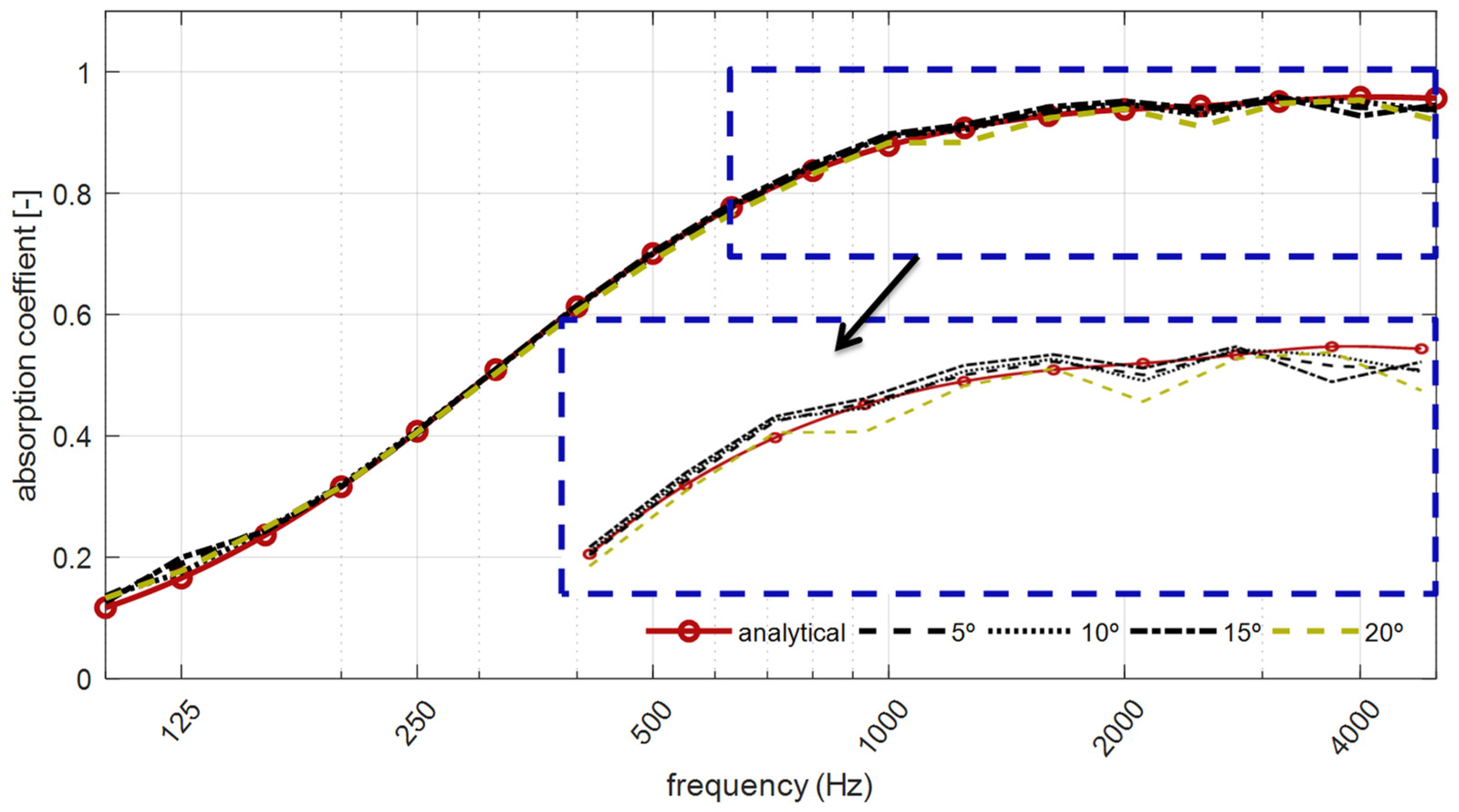
3.4.1. Paris Integration Domain

| Angles Range [°] | Weight at Paris’ Integration [%] |
|---|---|
| 45 | 8.8 |
| 55 | 8.2 |
| 30–60 | 57.6 |
| 15–75 | 90.1 |
| 05–85 | 100.0 |
| 10–80 1 | 100.0 |
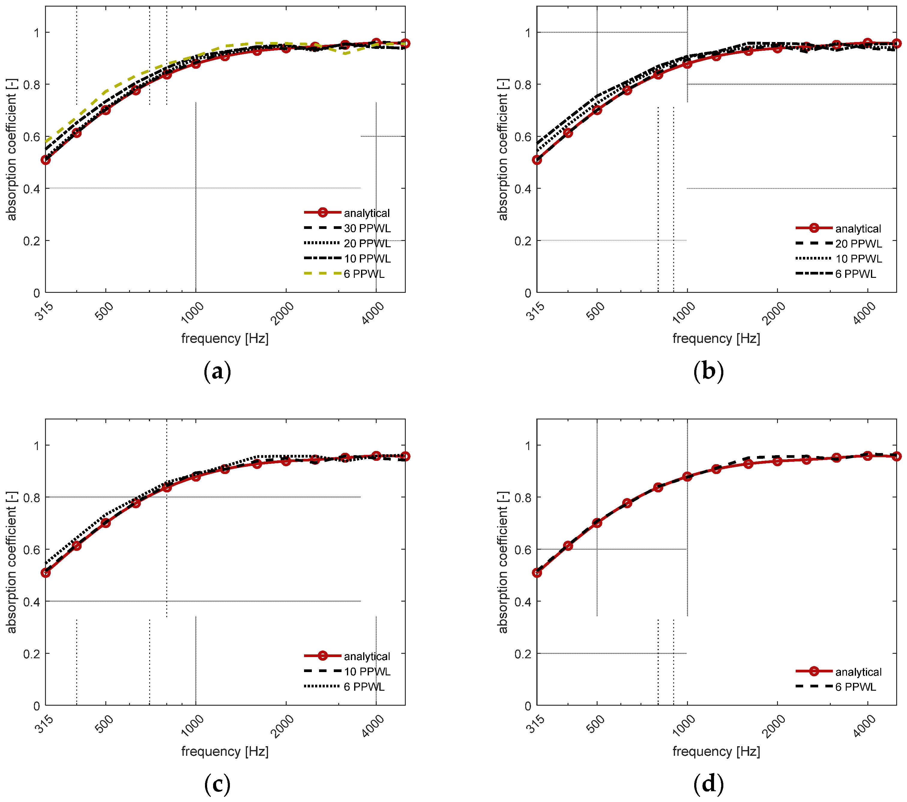
3.4.2. Minimum PPWL
3.4.3. Domain Dimensions
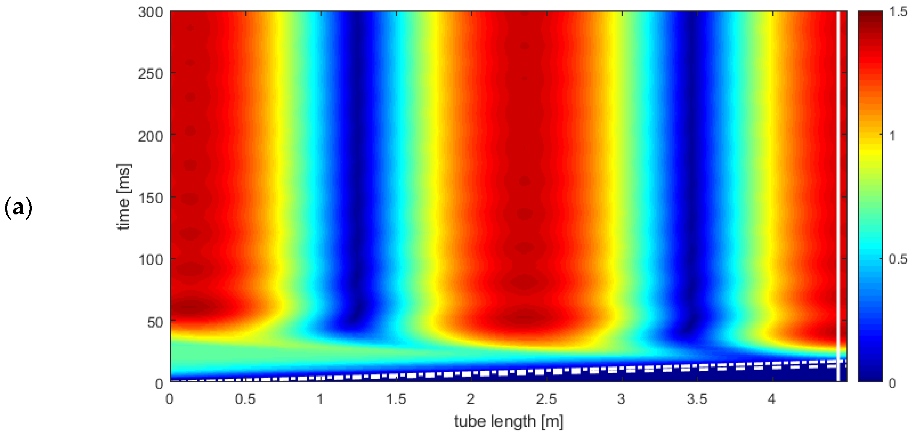
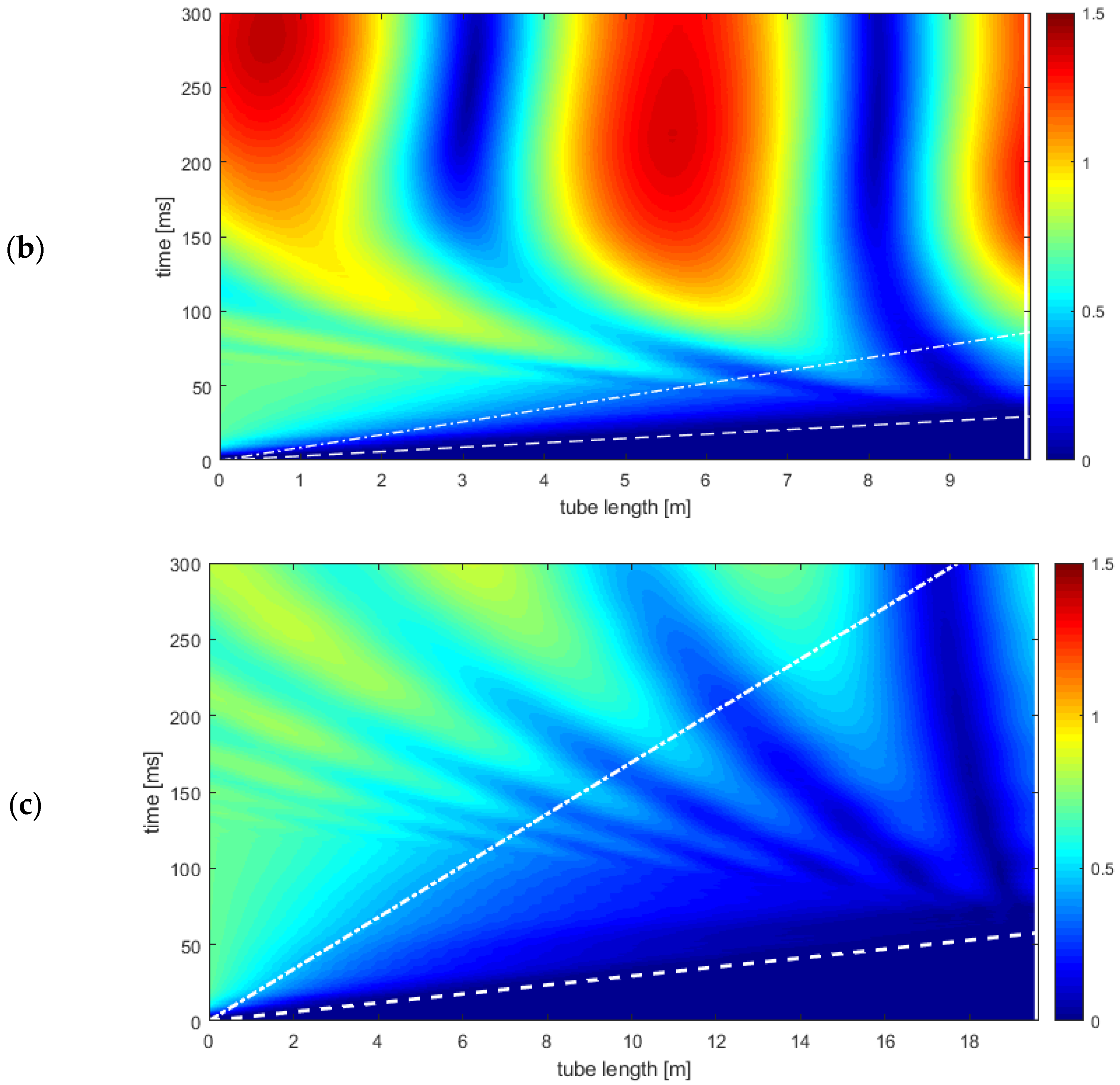
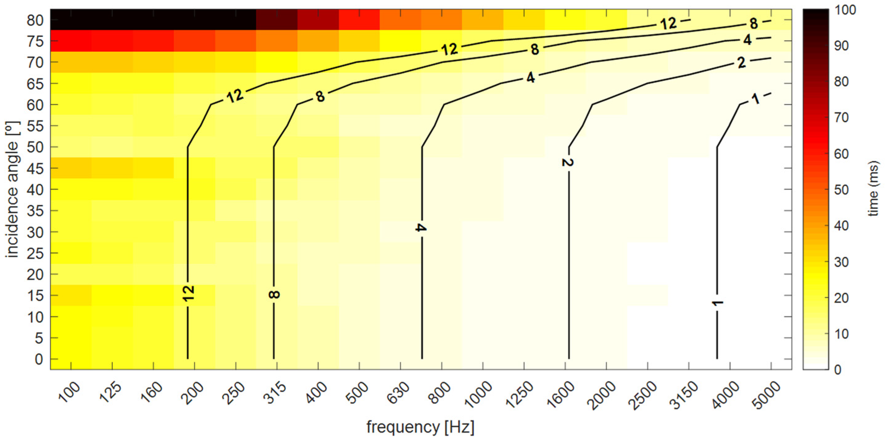
3.4.4. Propagation Time
3.4.5. Computing Time
4. Conclusions
Author Contributions
Funding
Institutional Review Board Statement
Informed Consent Statement
Data Availability Statement
Conflicts of Interest
References
- Attenborough, K. Acoustical characteristics of porous materials. Phys. Rep. 1982, 82, 179–227. [Google Scholar] [CrossRef]
- Biot, M.A. Theory of propagation of elastic waves in a fluid-saturated porous solid. I. Low-frequency range. J. Acoust. Soc. Am. 1956, 28, 168–178. [Google Scholar] [CrossRef]
- Biot, M.A. Theory of propagation of elastic waves in a fluid-saturated porous solid. II. Higher frequency range. J. Acoust. Soc. Am. 1956, 28, 179–191. [Google Scholar] [CrossRef]
- Delany, M.E.; Bazley, E.N. Acoustical properties of fibrous absorbent materials. Appl. Acoust. 1970, 3, 105–116. [Google Scholar] [CrossRef]
- Fellah, Z.E.A.; Depollier, C. Transient acoustic wave propagation in rigid porous media: A time-domain approach. J. Acoust. Soc. Am. 2000, 107, 683–688. [Google Scholar] [CrossRef] [PubMed]
- Fellah, M.; Fellah, Z.E.A.; Depollier, C. Generalized hyperbolic fractional equation for transient-wave propagation in layered rigid-frame porous materials. Phys. Rev. E 2008, 77, 016601. [Google Scholar] [CrossRef] [PubMed]
- Lafarge, D.; Lemarinier, P.; Allard, J.F.; Tarnow, V. Dynamic compressibility of air in porous structures at audible frequencies. J. Acoust. Soc. Am. 1997, 102, 1995–2006. [Google Scholar] [CrossRef]
- Johnson, D.L.; Koplik, J.; Dashen, R. Theory of dynamic permeability and tortuosity in fluid-saturated porous media. J. Fluid Mech. 1987, 176, 379–402. [Google Scholar] [CrossRef]
- Jaouen, L.; Gourdon, E.; Glé, P. Estimation of all six parameters of Johnson-Champoux-Allard-Lafarge model for acoustical porous materials from impedance tube measurements. J. Acoust. Soc. Am. 2020, 148, 1998–2005. [Google Scholar] [CrossRef]
- Niskanen, M.; Groby, J.-P.; Duclos, A.; Dazel, O.; Le Roux, J.C.; Poulain, N.; Huttunen, T.; Lähivaara, T. Deterministic and statistical characterization of rigid frame porous materials from impedance tube measurements. J. Acoust. Soc. Am. 2017, 142, 2407–2418. [Google Scholar] [CrossRef]
- Cortis, A. Dynamic Acoustic Parameters of Porous Media. Ph.D. Thesis, Technische Universiteit Delft, Delft, The Netherlands, 2002. [Google Scholar]
- Horoshenkov, K.V.; Hurrell, A.; Groby, J.-P. A three-parameter analytical model for the acoustical properties of porous media. J. Acoust. Soc. Am. 2019, 145, 2512–2517. [Google Scholar] [CrossRef]
- Kosten, C.W.; Zwikker, C. Sound Absorbing Materials; Elsevier: Amsterdam, The Netherlands, 1949. [Google Scholar]
- Escolano, J.; Pueo, B. Acoustic equations in the presence of rigid porous materials adapted to the finite-difference time-domain method. J. Comput. Acoust. 2007, 15, 255–269. [Google Scholar] [CrossRef]
- Wilson, D.K.; Collier, S.L.; Ostashev, V.E.; Aldridge, D.F.; Symons, N.P.; Marlin, D.H. Time-domain modeling of the acoustic impedance of porous surfaces. Acta Acust. United Acust. 2006, 92, 965–975. [Google Scholar]
- Wilson, D.K. Simple, relaxational models for the acoustical properties of porous media. Appl. Acoust. 1997, 50, 171–188. [Google Scholar] [CrossRef]
- Van Renterghem, T.; Botteldooren, D. Numerical evaluation of sound propagating over green roofs. J. Sound Vib. 2008, 317, 781–799. [Google Scholar] [CrossRef]
- Ferreira, N.; Hopkins, C. Using finite-difference time-domain methods with a Rayleigh approach to model low-frequency sound fields in small spaces subdivided by porous materials. Acoust. Sci. Technol. 2013, 34, 332–341. [Google Scholar] [CrossRef]
- Suzuki, H.; Omoto, A.; Fujiwara, K. Treatment of boundary conditions by finite difference time domain method. Acoust. Sci. Technol. 2007, 28, 16–26. [Google Scholar] [CrossRef]
- Zhao, J.; Chen, Z.; Bao, M.; Sakamoto, S. Prediction of sound absorption coefficients of acoustic wedges using finite-difference time-domain análisis. Appl. Acoust. 2019, 155, 428–441. [Google Scholar] [CrossRef]
- Alomar, A.; Dragna, D.; Galland, M.-A. Time-domain simulation of a flow duct with extended-reacting acoustic liners. Eforum Acusticum 2020, 407–409. [Google Scholar]
- Dragonetti, R.; Ianniello, C.; Romano, R. The use of an optimization tool to search non-acoustic parameters of porous materials. In Proceedings of the 33rd International Congress and Exposition on Noise Control Engineering, Prague, Czech Republic, 22–25 August 2004; pp. 3171–3177. [Google Scholar]
- Hamet, J.-F.; Berengier, M. Acoustical Chaacteristics of Porous Pavements: A New Phenomenological Model. In Proceedings of the 1993 International Congress on Noise Control Engineering—Internoise 93—People versus Noise, Leuven, Belgium, 24–26 August 1993. [Google Scholar]
- Leclaire, P.; Dupont, T.; Sicot, O.; Gong, X.-L. Propriétés acoustiques des matériaux poreux saturés d’air et théorie de Biot. J. D’acoustique 1990, 3, 29–38. [Google Scholar]
- Dragonetti, R.; Ianniello, C.; Romano, R.A. The evaluation of intrinsic non-acoustic parameters of polyester fibrous materials by an optimization procedure. In Proceedings of the 6th European Conference on Noise Control, Tampere, Finland, 30 May–1 June 2006. [Google Scholar]
- Moufid, I.; Matignon, D.; Roncen, R.; Piot, E. Energy analysis and discretization of the time-domain equivalent fluid model for wave propagation in rigid porous media. J. Comput. Phys. 2022, 451, 110888. [Google Scholar] [CrossRef]
- Wang, H.; Hornikx, M. Extended reacting boundary modeling of porous materials with thin coverings for time-domain room acoustic simulations. J. Sound Vib. 2023, 548, 117550. [Google Scholar] [CrossRef]
- ISO 10534-2:1998; Acoustics—Determination of Sound Absorption Coefficient and Impedance in Impedance Tubes—Part 2: Transfer-Function Method. International Organization for Standardization: Geneva, Switzerland, 1998.
- Kuttruff, H. Acoustics: An Introduction; CRC Press: Boca Raton, FL, USA, 2007. [Google Scholar]
- Kane, Y.E.E. Numerical solution of initial boundary value problems involving Maxwell’s equations in isotropic media. IEEE Trans. Antennas Propag. 1966, 14, 302–307. [Google Scholar] [CrossRef]
- Taflove, A.; Hagness, S.C. Computational Electrodynamics: The Finite-Difference Time-Domain Method, 3rd ed.; Artech House Publishers: Norwood, MA, USA, 2005. [Google Scholar]
- Schneider, J.B. Understanding the Finite-Difference Time-Domain Method; School of Electrical Engineering and Computer Science Washington State University: Pullman, DC, USA, 2010; Volume 28. [Google Scholar]
- ISO 10534-1:1996; Acoustics—Determination of Sound Absorption Coefficient and Impedance in Impedance Tubes—Part 1: Method Using Standing Wave Ratio. International Organization for Standardization: Geneva, Switzerland, 1996.
- Kuttruff, H. Room Acoustics, 5th ed.; Spon Press: London, UK, 2009. [Google Scholar]
- Cox, T.J.; D’antonio, P. Acoustic Absorbers and Diffusers: Theory, Design and Application; CRC Press: Boca Raton, FL, USA, 2009. [Google Scholar]
- ISO 354:2003; Acoustics—Measurement of Sound Absorption in a Reverberation Room. International Organization for Standardization: Geneva, Switzerland, 2003.
- Pereira, M.; Mareze, P.; Godinho, L.; Amado-Mendes, P.; Ramis, J. Proposal of numerical models to predict the diffuse field sound absorption of finite sized porous materials—BEM and FEM approaches. Appl. Acoust. 2021, 180, 108092. [Google Scholar] [CrossRef]
- Tormos, R.; Fernández, A.; Ramis-Soriano, J.; Rico, S.; Vicente, J. Nuevos materiales absorbentes acústicos obtenidos a partir de restos de botellas de plástico. Mater. Construcción 2011, 61, 547–558. [Google Scholar]


| [-] | [Pa] | [Pa·s] | [-] | th. [mm] |
|---|---|---|---|---|
| 1.0953957103 1 | 9 × 10⁻¹⁰ | 18 × 10−6 | 0.98 | 50 |
| PPWL | Rounded | Not Rounded | Rounded | Not Rounded |
|---|---|---|---|---|
| 6 | 1.0000017548 | 1.0000017548 | 13,833 | 13,790 |
| 10 | 1.0390070343 | 1.0301187897 | 18,225 | 18,582 |
| 20 | 1.0419824982 | 1.0337904358 | 18,395 | 18,728 |
| 30 | 1.0826280975 | 1.0741842651 | 19,084 | 19,429 |
| 40 | 1.1039675140 | 1.0953920746 | 19,450 | 19,800 |
| low. freq. model | 1.0953957103 | 19,800 | ||
| 1D PPWL | 2D PPWL | |||||
|---|---|---|---|---|---|---|
| 30 | 30 | 20 | 10 1 | 6 1 | ||
| 20 | 20 | 10 1 | 6 1 | |||
| 10 | 10 1 | 6 1 | ||||
| 6 | 6 1 | |||||
Disclaimer/Publisher’s Note: The statements, opinions and data contained in all publications are solely those of the individual author(s) and contributor(s) and not of MDPI and/or the editor(s). MDPI and/or the editor(s) disclaim responsibility for any injury to people or property resulting from any ideas, methods, instructions or products referred to in the content. |
© 2024 by the authors. Licensee MDPI, Basel, Switzerland. This article is an open access article distributed under the terms and conditions of the Creative Commons Attribution (CC BY) license (https://creativecommons.org/licenses/by/4.0/).
Share and Cite
Iglesias, P.C.; Godinho, L.; Redondo, J. Numerical Equivalent Acoustic Material for Air-Filled Porous Absorption Simulations in Finite Different Time Domain Methods: Design and Comparison. Appl. Sci. 2024, 14, 1222. https://doi.org/10.3390/app14031222
Iglesias PC, Godinho L, Redondo J. Numerical Equivalent Acoustic Material for Air-Filled Porous Absorption Simulations in Finite Different Time Domain Methods: Design and Comparison. Applied Sciences. 2024; 14(3):1222. https://doi.org/10.3390/app14031222
Chicago/Turabian StyleIglesias, P. C., L. Godinho, and J. Redondo. 2024. "Numerical Equivalent Acoustic Material for Air-Filled Porous Absorption Simulations in Finite Different Time Domain Methods: Design and Comparison" Applied Sciences 14, no. 3: 1222. https://doi.org/10.3390/app14031222