
Establishment of a Pressure Variation Model for the State Estimation of an Underwater Vehicle
by
 , , , , and
Ji-Hye Kim
1 ,
,
Thi Loan Mai
1 ,
,
Aeri Cho
1,
Namug Heo
1,
Hyeon Kyu Yoon
1,*,
Jin-Yeong Park
2 and
Sung-Hoon Byun
2 1
Department of Smart Ocean Mobility Engineering, Changwon National University, Changwon 51140, Republic of Korea
2
Korea Research Institute of Ships and Ocean Engineering (KRISO), Daejeon 34103, Republic of Korea
*
Author to whom correspondence should be addressed.
Appl. Sci. 2024, 14(3), 970; https://doi.org/10.3390/app14030970
Submission received: 28 December 2023
/
Revised: 20 January 2024
/
Accepted: 22 January 2024
/
Published: 23 January 2024
(This article belongs to the Special Issue Recent Advances in Underwater Vehicles)
Abstract
:This study presents a pressure variation model (PVM) derived from the regression analysis of dynamic pressure computed through numerical analysis to estimate the velocity of underwater vehicles. Furthermore, the drift angle estimation algorithm was developed using predicted velocities from PVM and pressure sensor differences. This approach estimates the single-motion states of underwater vehicles, such as straight, turning, and gliding. Furthermore, it confirms the viability of state estimation even in multiple motions involving turning and gliding motion with a drift angle and spiral motion. The comparison with numerical analysis results validated prediction accuracy within 15%.
1. Introduction
Recently, significant progress has been achieved in unmanned underwater vehicles (UUVs) and related core technologies serving various purposes such as oceanographic data collection, exploration, reconnaissance, surveillance, and more. This progress has increased the demand for fundamental technological advancements in structural design, propulsion systems, control mechanisms, underwater docking, and underwater navigation technologies for these UUVs. Especially in underwater environments, the precise and rapid estimation of their state is crucial for mission execution and the subsequent analysis of acquired underwater data by unmanned underwater vehicles. Numerous methods exist to estimate the motion state of these vehicles, and research inspired by fish lateral line systems (LLSs) has developed actively. It is well known that fish can detect flow velocity and pressure in the surrounding flow field through the LLS. Inspired by the exceptional performance of the LLS in fish, there has been significant interest in research on artificial lateral line systems (ALLSs).
Chambers et al. (2014) presented a data-driven methodology enabling the simultaneous recording of 3D pressure signals while in motion and examined flow features using a sensor array placed inside a fish-shaped head [1]. Levi et al. (2014) introduced a strategy for an airfoil-shaped UUV to estimate flow properties using a bio-inspired, multi-modal artificial lateral line and demonstrate their use in feedback control. They showcased these strategies using a robotic prototype with a multi-modal artificial later line, highlighting distributed flow sensing and closed-loop control capabilities [2]. Nataliya et al. (2016) carried out investigations using an artificial later line (ALL) array for estimating bulk flow velocity and angle, demonstrating its accuracy in measuring these parameters even in river conditions, with an average velocity estimation error of 14 cm/s [3]. Wang et al. (2016) utilized an ALL for the precise evaluation of a swimming robot, proposing a nonlinear predictive model based on pressure analysis and motion kinematics data [4]. Xu and Mohseni (2016) introduced a sensor system that uses differential pressure sensors for precise measurements, demonstrating its ability to estimate hydrodynamic force and detect nearby walls by analyzing pressure distribution [5]. Ali et al. (2017) investigated optimal 3D design strategies for dipole source characterization using ALLS. They proposed strategies to overcome design limitations, cooperatively explored ALL swarms, and analyzed the trade-offs between sensor quantity and characterization accuracy [6]. Yen et al. (2018) focused on measuring the hydrodynamic pressure of a robotic fish during its movements near a straight wall and using the pressure data for feedback control of its motion [7]. Liu et al. (2018) explored improving the ALLS in underwater technology using a cylindrical carrier. This study examined biomechanics, developed optimal sensor distribution, and validated the system through experiments, offering effective methods for flow velocity estimation and obstacle identification [8]. Zheng et al. (2018) examined the hydrodynamic features of the reverse KVS (Kármán vortex street)-like vortex wake with an ALLS. Furthermore, they demonstrated the efficiency and viability of using an ALL for local sensing in nearby underwater robots [9]. Zheng et al. (2020) investigated the state estimation of a swimming robotic fish across various motions using a pressure variation (PV) model and regression analysis. Additionally, they proposed a trajectory estimation method and demonstrated it with minimal errors [10].
This paper proposes a pressure variation model (PVM) designed to predict the motion state, particularly the speed and direction, of underwater vehicles. Computational fluid dynamics (CFD), known for its precision and adaptability in simulating motion, is utilized to construct this model. Additionally, dynamic pressures observed during 3D motions, such as straight, turning, gliding, and spiral motions, are measured using pressure sensors arranged on the top, bottom, left, and right sides of arbitrary-shaped underwater vehicles. After determining the coefficients through regression analysis based on the acquired data, the PVM can estimate the velocity, direction, and localization of underwater vehicles.
2. Methodology and Results
2.1. Test Model
The autonomous underwater vehicle (AUV) used in this study is a slender body by REMUS. The primary dimensions are 1.345 m in length and 0.191 m in diameter (Table 1).
Figure 1 shows the shape of the AUV and the arrangement of 0.01 m diameter pressure sensors (red circles with numbers) located on the front and sides. Each of the pressure sensors is named and positioned as described in the bottom left of Figure 1, with R, L, T and B representing the pressure sensors on the right (starboard), left (port), top, and bottom sides, respectively. Through prior research, it was confirmed that placing sensors in locations with significant changes in pressure with speed leads to a higher accuracy in predicting the speed and drift angle of AUVs. Therefore, pressure sensors were arranged at the front of the vehicle, considering the size of the pressure sensors, and 11 sensors were arranged at appropriate intervals.
2.2. Pressure Variation Model (PVM)
Zheng et al. (2020) proposed PV models correlating motion parameters with pressure variations (PVs) observed during the movement of a robotic fish. According to Lighthill’s discussion [11], the hydrodynamic PVs across the body surface of the robotic fish can be approximated by the unsteady Bernoulli equation, assuming an irrotational flow and the absence of a boundary layer. Here, the linearized velocity potential is related to the robot fish’s body with the translational velocity U, the pitch angle θ, and body sway angular velocity ω, forming the expression of the PV model. Then, the dynamic pressure, Pd, can be expressed as shown in Equation (1), and the coefficients for each motion are derived through linear regression analysis using experimental data.
However, this model has limitations. It requires the prior identification of the body’s movements and using coefficients specific to each motion, making it challenging to apply to multiple movements. So, in this study, the PVM was designed to utilize identical coefficients for the entire motion range, and it was structured to encompass both velocity estimation algorithms and state estimation algorithms.
2.2.1. Velocity Estimation
First, to estimate the velocity U of the AUV, a single equation (Equation (2)) is used, similar to Zheng et al. (2020), but the same coefficients of PVM are set for all motion conditions. Representative captive model tests called PMM (planar motion mechanism) determine non-dimensional hydrodynamic maneuvering coefficients. Following the model’s path and acquiring forces and moments under specific yaw and sway conditions, it measures hydrodynamic forces and estimates the hydrodynamic coefficient.
where α and β represent the drift angle on the vertical and horizontal plane, and q and r denote the angular velocities on the vertical and horizontal plane. Figure 2 depicts the definitions of these variables and Figure 3 depicts the specific definitions of each founded motion. We employed numerical analysis to predict the dynamic pressure in three motion conditions (straight, gliding, and turning). Based on these results, we derived PVM coefficients (C1~C6) through linear regression. At this point, the velocity and drift angles are known, and the angular velocity is assumed to be measured from the inertial sensor.
Table 2 depicts the test conditions for obtaining PVM coefficients, and the performance of the acquired PVM evaluates the coefficient of determination R2 and the mean absolute error (MAE) between the estimated value and the measured one.
Here, n is the number of test cases, Pd,est is the estimated hydrodynamic pressure using Equation (2), and Pd is the calculated hydrodynamic pressure using CFD. Table 3 shows the coefficients of determination obtained from regression analysis for each motion condition concerning sensor 1 through 11. Figure 4 shows the overall process of AUV state estimation in this paper, and the details about the numerical analysis are described in Section 2.3.
Equation (2) enables us to predict the sum of the square of the drift angle. Still, it requires a second step to overcome the limitation of being able to separate individual components. Here, the difference in dynamic pressure between sensors located at the top and bottom, right and left sides, was formulated with the following equations (Equations (7) and (8)) and coefficients (D1~D4) obtained through linear regression using the velocity predicted at the previous step. Furthermore, as the AUV is axisymmetric, the coefficients for the pressure difference between sensors located at the top, bottom, right, and left sides can be equally applied.
Then, Table 4 shows the coefficients of determination obtained from regression analysis for each motion condition concerning sensor 1 through 11.
Based on the results in Table 3, it can be confirmed that sensors 4 to 7 exhibited better estimation performance for velocity estimation, and based on the results in Table 4, it can be confirmed that sensors 2 to 5 showed reasonable performance for drift angle estimation. Then, sensors 4 to 7 were used for velocity estimation, and sensors 2 to 5 were utilized for drift angle estimation to construct the inverse matrix. The PVM coefficients for each pressure sensor obtained using regression analysis are shown in Table 5, and details on the state estimation process are described in Section 2.2.2.
2.2.2. State Estimation
To estimate velocity as the initial step from the established PVM, an inverse matrix is constructed using the dynamic pressures of four sensors and its regression coefficients obtained from the previous step. Based on the last analysis, the regression outcomes select pressure sensors 4 to 7, and the second subscript indices of the PVM coefficients in Equation (9) represent the sensor number. The estimated velocities for straight, turning, and gliding motions are presented in Table 6, Table 7 and Table 8, demonstrating accurate predictions of the AUV’s velocity.
For straight, turning, and gliding motions, it is confirmed that the maximum error is within 1%, 2.5%, and 7%, respectively, demonstrating accurate velocity predictions. Furthermore, utilizing the predicted velocity and dynamic pressure, the drift angles are estimated through Equation (11) to Equation (12), and the second subscript indices of the PVM coefficients in Equations (10) and (11) represent the sensor number. Based on the previous regression analysis, pressure sensors 2 to 5 were used to estimate the drift angles (, and the relative error for straight, turning, and gliding motions is provided in Table 9, Table 10 and Table 11.
For straight and turning motions with zero drift angles, the state estimation results indicate proximity to zero across all velocity and angular velocity conditions, affirming accurate predictions. Moreover, during the gliding motion, when the angle of attack varied from 0 to −30 degrees in intervals of 5 degrees at speeds ranging from 1 to 4 knots, the error stayed within 10%, excluding the low-speed 1 knot condition. The numerical results (Section 2.4) indicate that as the speed increases, the pressure variations corresponding to the drift angle become more pronounced, leading to higher prediction accuracy. Conversely, under low-speed conditions, the pressure variations are relatively small, resulting in lower prediction accuracy. Additionally, this confirms that the drift angle was well-predicted, closely approximating zero.
Previously, regression coefficients were derived from single-motion data, enabling the prediction of the velocity and drift angles of the AUV using an array of pressure sensors. As the objective of this study was to apply this PVM to estimate the state during multiple motions, the aim was to validate the PVM and state estimation methods based on the numerous motion conditions listed in Table 12. Figure 5 depicts the definitions for each motion.
For the turning with drift motion, velocity predictions were made for angular velocities between 10 and 30 rad/s and drift angles between 0 and 20 deg at a designed speed of 3 knots. With an angle of attack of zero, the model predicts velocities within approximately 10% across all angular velocity and drift angle conditions (Table 13).
For the gliding with drift motion, velocity predictions were made for angle of attacks between −10 and −20 deg and drift angles between 0 and 20 deg, at speeds of 1.5 and 3 knots. Then, the predicted velocity was within approximately 3% across all drift angle conditions (Table 14). Velocity predictions were made for spiral motion at an angle of attack between −10 and −30 degrees and angular velocities between 10 and 30 rad/s, at a design speed of 3 knots. The predicted velocity was accurate within 12.5% for all angles and angular velocities (Table 15). Then, the model estimates the drift angles using the previously predicted velocity and pressure difference data. At the design speed of 3 knots, the angle of attack for the turning with drift motion is expected to be near zero. For the drift angle, except for the condition at 20 deg when the angular velocity is 10 deg/s, the maximum error is approximately 8%. For the 20 deg drift angle with an angular velocity of 10 rad/s, the prediction showed a higher error rate of about 20%, due to the slightly lower accuracy in the earlier velocity prediction (Table 16).
Drift angles practice for speeds of 1.5 and 3 knots, with the angle of attacks between −10 and −20 deg and drift angles between 0 and 30 deg for gliding with drift motion. The drift angles predict within approximately 10% across all drift angle conditions (Table 17). In addition, for spiral motion, drift angles predict angles of attack between −10 and −30 deg and angular velocities between 10 and 30 deg, at a design speed of 3 knots. The angle of attack was predicted within 15% across all drift angle conditions, except for the condition at −20 deg when the angular velocity is 10 deg/s. For the −20 deg angle of attack with angular velocity 10 rad/s, the prediction showed a higher error rate of about 40% due to the relatively lower accuracy in the earlier velocity prediction (Table 18).
Ultimately, using the PVM constructed through the regression analysis based on CFD results, the estimated states of the AUV predict velocities and drift angles within the target range initially expected, with an error margin of 15% or less, similar to the prediction accuracy level of advanced research groups [10]. However, during the estimation of states in multiple motions, certain conditions display relatively high errors in the estimated drift angles, and it appears that there might be some discrepancies due to the absence of terms in the PVM that account for the correlation between drift angle and angular velocity. Therefore, further improvements in the PVM are needed to correct these issues.
2.3. Flow Simulation
2.3.1. Governing Equation and Boundary Condition
To examine the unsteady flow around the underwater vehicle, every cell in the control volume adheres to the governing equations, which encompass the continuity equation, formulated as:
and the Reynolds-averaged Navier–Stokes (RANS) momentum equation, expressed as:
where u, P, and F denote the velocity, pressure, and external force, respectively. A commercial program, STAR-CCM+ ver. 13.06.012, was used for the flow analysis of the underwater vehicle in specific motions. The diffusion and convection terms of the governing equations discretize to second-order accuracy, and the velocity and pressure were analyzed using the SIMPLE (semi-implicit method for pressure-linked equations) algorithm. A turbulence model applying the k-ω SST (shear stress transport) model and the wall functions uses the submerged body’s boundary condition.
2.3.2. Simulation Set-Up
The computational domain adheres to the recommended ITTC (International Towing Tank Conference) procedure (2011) [12], ensuring it is sufficiently large to prevent backflow or reflection. Physical conditions apply the boundary domain with a velocity inlet defined at the fluid domain’s upstream, top, bottom, and sidewalls, and a pressure outlet imposing the downstream. A no-slip wall surrounds the AUV, while an elliptical cover serves as an overset region to facilitate the AUV’s movement in straight, turning, gliding, and spiral motions. Mesh generation was automated using the cut-cell method for volume and surface, employing a trimmed cell mesher for volume grids and a surface remesher for high-quality surface mesh. The AUV encompasses a boundary layer consisting of 10 layers of prismatic cells. The simulation consistently maintained a y+ value below one, refining the conditions around the AUV’s trajectory using volumetric control to enhance calculation precision. Figure 6 illustrates the computational mesh, boundary conditions, and boundary domain for straight, turning, and gliding motions. The AUV simulation was conducted at a water depth of 7 m from the surface for straight and turning motions and at the same depth for gliding motion.
2.4. Numerical Results
Figure 7, Figure 8, Figure 9, Figure 10, Figure 11 and Figure 12 illustrate the pressure for each motion condition obtained through the numerical analysis to find the PVM coefficients. The pressure values used for the regression analysis were obtained by subtracting the hydrostatic pressure from the gauge pressure, which was considered sufficiently converged at a physical time of 2.5 s. We summarized the results for sensors 2 to 7, selected based on the coefficient of determination and MAE among pressure sensors 1 to 11. Sensors 8 to 11 on the parallel body part exhibited pressure characteristics similar to seshinsor 7; hence, we excluded their results. Figure 7 presents the calculated pressure results at the positions of each sensor of the AUV during straight motion. For straight motion, the pressure characteristics of only the left sensor concerning velocity are shown since the pressures for all sensors are equal. The pressure differences among sensors are approximately 500 Pa across all velocity conditions, demonstrating a distinct pressure characteristic concerning velocity. Furthermore, it can be observed that the pressure clearly varies in proportion to the square of the velocity.
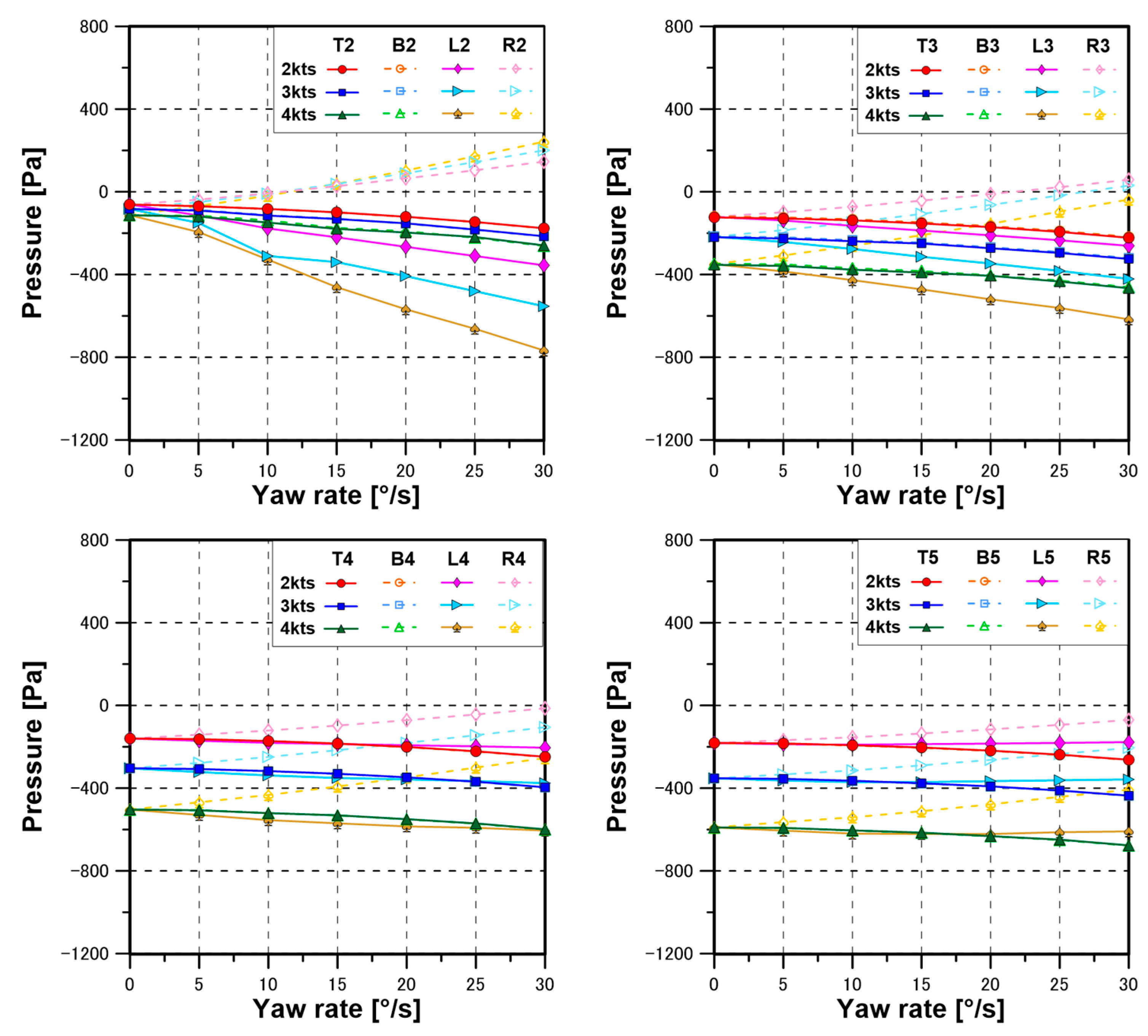
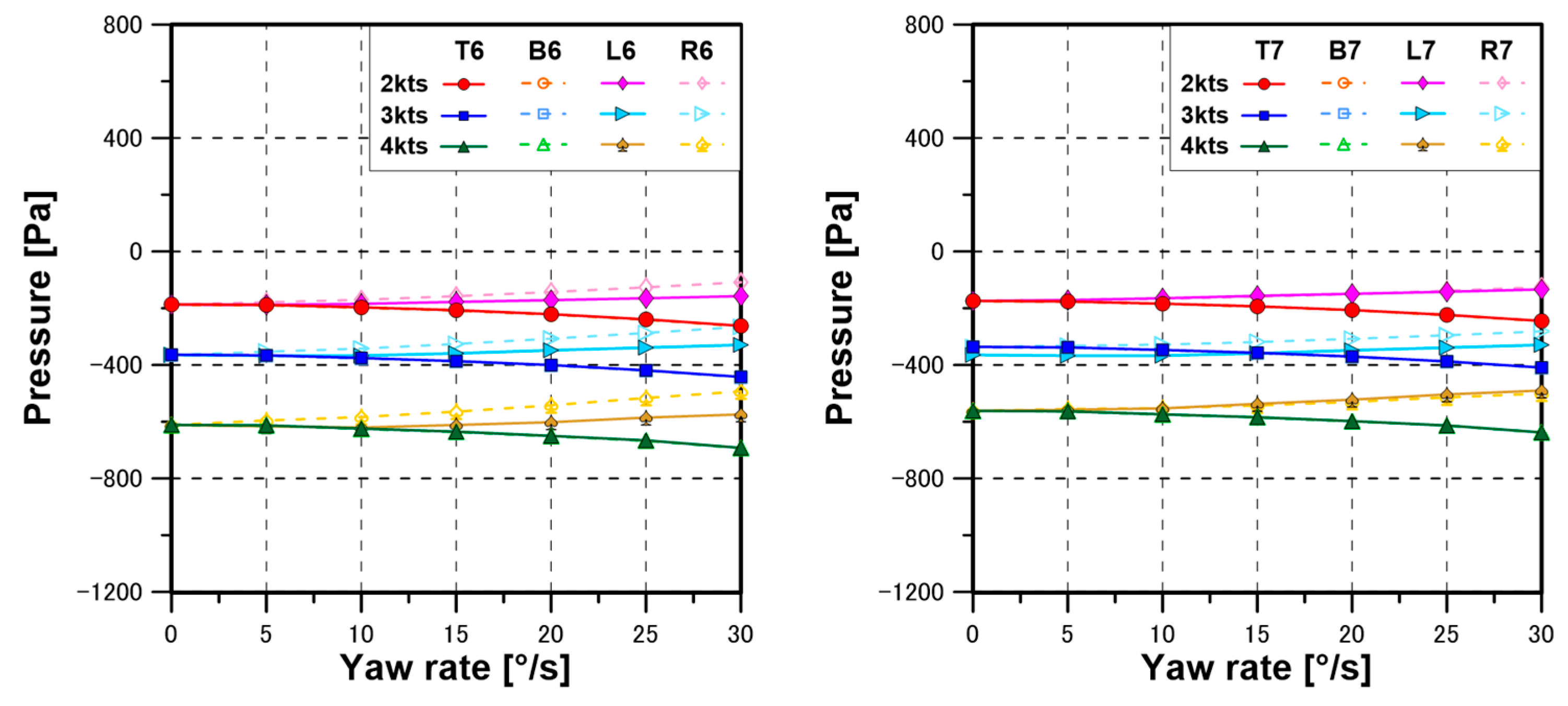
Figure 8 shows the pressure characteristics of the top, bottom, left, and right sensors concerning velocity and angular velocity during turning motion. In this case, only right turns were considered, resulting in pressure differences between the left and right sensors, while the pressure between the top and bottom sensors remained consistent. The disparity in pressure between the left and right sensors notably appears more pronounced in the front sensors, with substantial changes in the AUV’s shape. Then, it seems logical to estimate the drift angle using the pressure data from front-positioned sensors. Figure 9 shows the pressure characteristics of sensors located on the AUV’s top, bottom, left, and right sides concerning drift angles during gliding motion at a design speed of 3 knots. Uniform pressures are confirmed at the left and right sensors, and differences are noticeable between the top and bottom sensors, with these differences becoming more pronounced as the sensors are positioned towards the front. The pressure values calculated from the upper sensors are higher than those from the lower sensors due to the negative angle of attack.
Figure 9.
Pressure on the array of sensors during gliding motion.


Figure 10 shows the pressure characteristics of the top, bottom, left, and right sensors concerning velocity and angular velocity during turning motion with drift angle. As the drift angle increases, the pressure difference between the left and right sensors becomes more significant, while higher angular velocities are associated with more minor pressure differences.
Figure 10.
Pressure on the array of sensors during turning motion with drift angle.
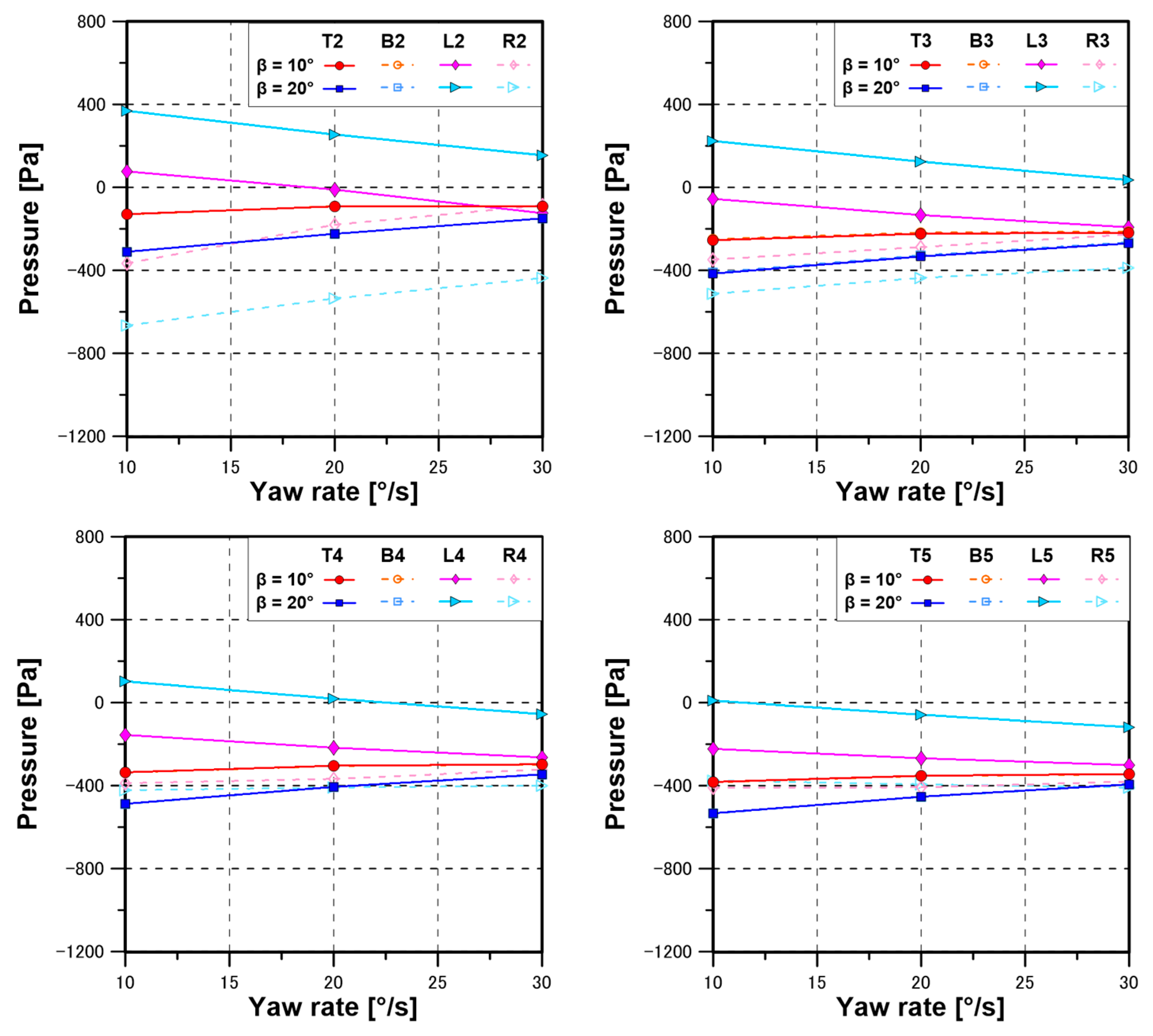

Figure 11 presents the pressure characteristics of the sensors concerning the drift angles during gliding motion with drift angle at a design speed of 3 knots. As drift angles increase, the pressure differences also increase. Moreover, as in the previous cases, it is noticeable that the pressure difference is more pronounced in the sensors located towards the front. Figure 12 shows the pressure characteristics of sensors concerning the angle of attack and angular velocities during spiral motion at a design speed of 3 knots. As the angle of attack and angular velocity increase, the pressure differences also increase.
Figure 11.
Pressure on the array of sensors during gliding motion with drift angle.
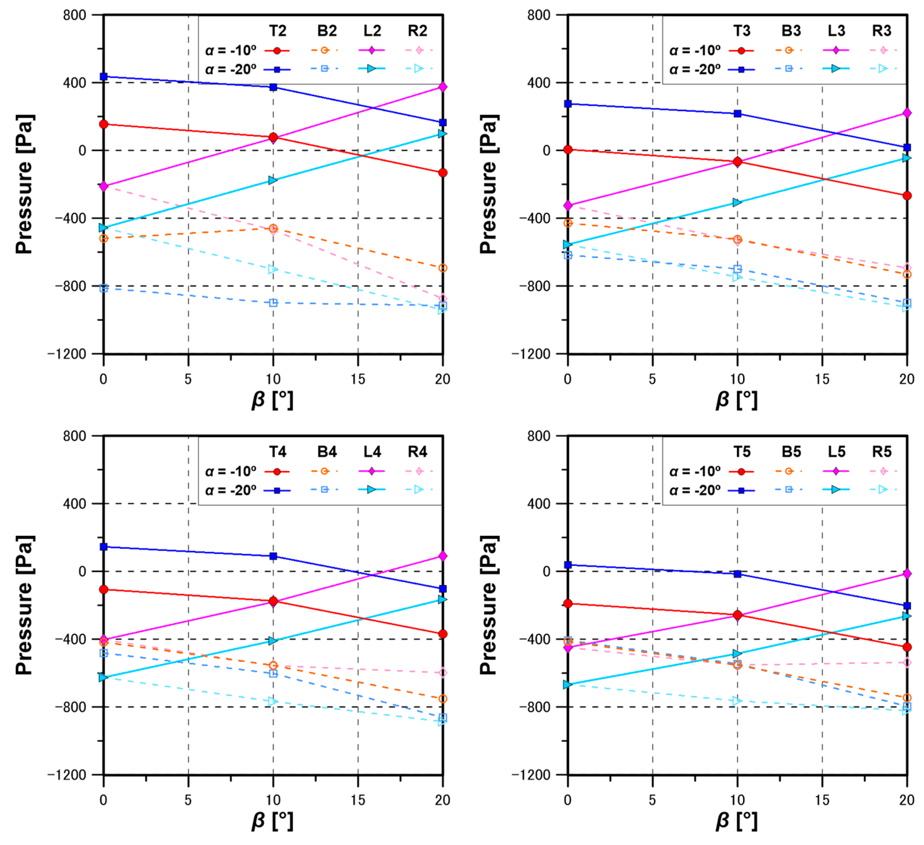
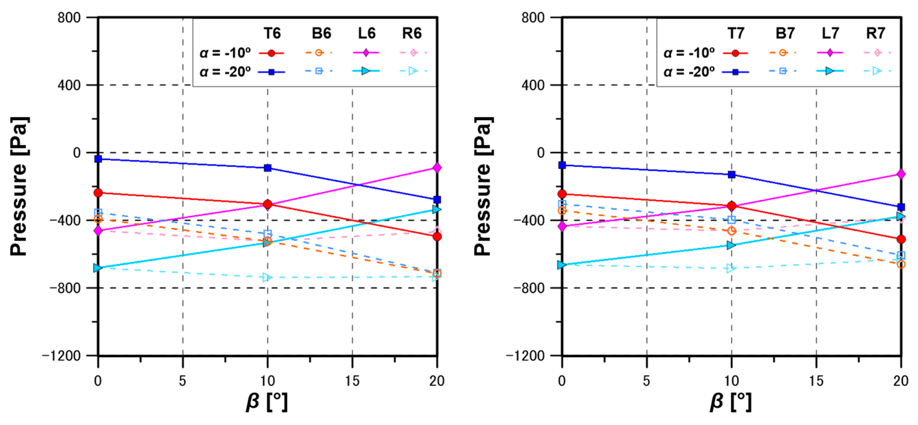
Figure 12.
Pressure on the array of sensors during spiral motion.

3. Conclusions
This study aimed to establish a pressure variation model (PVM) for the state estimation of the AUV based on dynamic pressure data obtained through numerical analysis. The study yielded the following results.
- The dynamic pressure characteristics were analyzed by numerical simulations for straight, turning, and gliding motions under speed, angular velocity, and angle of attack conditions.
- The coefficients for the PVM were derived by performing regression analysis on the dynamic pressure obtained from numerical simulations, considering the coefficient of determination and the MAE for evaluation.
- The state estimation algorithm was presented by combining the regression equations of the pressure sensors array to form an inverse matrix. Furthermore, it was validated for single and multiple motions, confirming the targeted prediction accuracy within 15%.
In this research process, it was confirmed that as the velocity of the AUV increases, the pressure difference becomes more pronounced, enhancing the accuracy of predicting both the speed and drift angle. Therefore, it is anticipated that the accuracy of estimating the state of the AUV will be higher when the size and speed of AUVs are larger than the present target. However, due to the concern about nonlinearity, such as the correlation between angular velocity and drift angle, potentially leading to a decrease in prediction accuracy, plans are in progress to further improve the PVM to address this issue. Additionally, in future research, we plan to validate the PVM based not only on pressure data obtained through the numerical analysis but also using pressure data acquired through experiments.
Author Contributions
Conceptualization, methodology and writing, J.-H.K. and H.K.Y.; CFD calculation, T.L.M.; data analysis, A.C. and N.H.; resources, J.-Y.P. and S.-H.B. All authors have read and agreed to the published version of the manuscript.
Funding
This research was supported by a grant from the Endowment Project of “Development of smart sensor technology for underwater environment monitoring”, funded by the Korea Research Institute of Ships and Ocean Engineering (PES4400) and the National Research Foundation of Korea (NRF) grant funded by the Korea government (MSIT) (NRF-2022R1A2C1093055).
Institutional Review Board Statement
Not applicable.
Informed Consent Statement
Not applicable.
Data Availability Statement
The raw data supporting the conclusions of this article will be made available by the authors on request.
Conflicts of Interest
The authors declare no conflicts of interest. The funders had no role in the design of the study; in the collection, analyses, or interpretation of data; in the writing of the manuscript, or in the decision to publish the results.
Abbreviations
| PVM | pressure variation model |
| UUVs | unmanned underwater vehicles |
| LLSs | lateral line systems |
| ALLSs | artificial lateral line systems |
| ALL | artificial lateral line |
| AUV | autonomous underwater vehicle |
| R, L, T, B | pressure sensor position: right (starboard), left (port), top, bottom |
| PVs | pressure variations |
| MAE | mean absolute error |
| CFD | computational fluid dynamics |
| EFD | experimental fluid dynamics |
| RANS | Reynolds-averaged Navier–Stokes |
| SIMPLE | semi-implicit method for pressure-linked equation |
| SST | shear stress transport |
| ITTC | International Towing Tank Conference |
References
- Chamber, L.D.; Akanyeti, O.; Venturelli, R.; Jezov, J.; Brown, J.; Kruusmaa, M.; Fiorini, P.; Megill, W.M. A fish perspective: Detecting flow features while moving using an artificial lateral line in steady and unsteady flow. J. R. Soc. Interface 2014, 11, 20140467. [Google Scholar] [CrossRef] [PubMed]
- Levi, D.V.; Francis, D.L.; Hong, L.; Xiaobo, T.; Derek, A.P. Distributed flow estimation and closed-loop control of an underwater vehicle with a multi-modal artificial lateral line. Bioinspir. Biomim. 2014, 10, 025002. [Google Scholar]
- Strokina, N.; Kamarainen, J.K.; Tuhtan, J.A.; Fuentes-Perez, J.F.; Kruusmaa, M. Joint estimation of bulk flow velocity and angle using a later line probe. IEEE Trans. Instrum. Meas. 2016, 65, 601–613. [Google Scholar] [CrossRef]
- Wang, W.; Li, Y.; Zhang, X.; Wang, C.; Chen, S.; Xie, G. Speed evaluation of a freely swimming robotic fish with an artificial lateral line. In Proceedings of the 2016 IEEE International Conference on Robotics and Automation (ICRA), Stockholm, Sweden, 16–21 May 2016; pp. 4737–4742. [Google Scholar]
- Xu, Y.; Mohseni, K. A pressure sensory system inspired by the fish lateral line: Hydrodynamic force estimation and wall detection. IEEE J. Ocean. Eng. 2016, 42, 532–543. [Google Scholar] [CrossRef]
- Ali, A.; Hong, L.; Montassar, A.S.; Kalyanmoy, D.; Xiaobo, T. Reliable underwater dipole source characteristics in 3D space by an optimally designed artificial lateral line system. Bioinspir. Biomim. 2017, 12, 036010. [Google Scholar]
- Yen, W.K.; Sierra, D.M.; Guo, J. Controlling a robotic fish to swim along a wall using hydrodynamic pressure feedback. IEEE J. Ocean. Eng. 2018, 43, 369–380. [Google Scholar] [CrossRef]
- Liu, G.; Wang, M.; Wang, A.; Wang, S.; Yang, T.; Malekian, R.; Li, Z. Research on flow field perception based on artificial lateral line sensor system. Sensors 2018, 18, 838. [Google Scholar] [CrossRef]
- Zheng, X.; Wang, C.; Fan, R.; Xie, G. Artificial lateral line based local sensing between two adjacent robotic fish. Bioinspir. Biomim. 2018, 13, 016002. [Google Scholar] [CrossRef] [PubMed]
- Zheng, X.; Wang, W.; Xiong, M.; Xie, G. Online state estimation of a fin-actuated underwater robot using artificial lateral line system. IEEE Trans. Robot. 2020, 36, 472–487. [Google Scholar] [CrossRef]
- Lighthill, J. Estimates of pressure differences across the head of a swimming clupeid fish. Philos. Trans. Biol. Sci. 1993, 341, 129–140. [Google Scholar]
- ITTC. ITTC-Recommended Procedures and Guidelines: Practical Guidelines for Ship CFD Application. Tech. Rep. 2011, 3, 1–18. [Google Scholar]
Figure 1.
AUV shape and pressure sensor position.
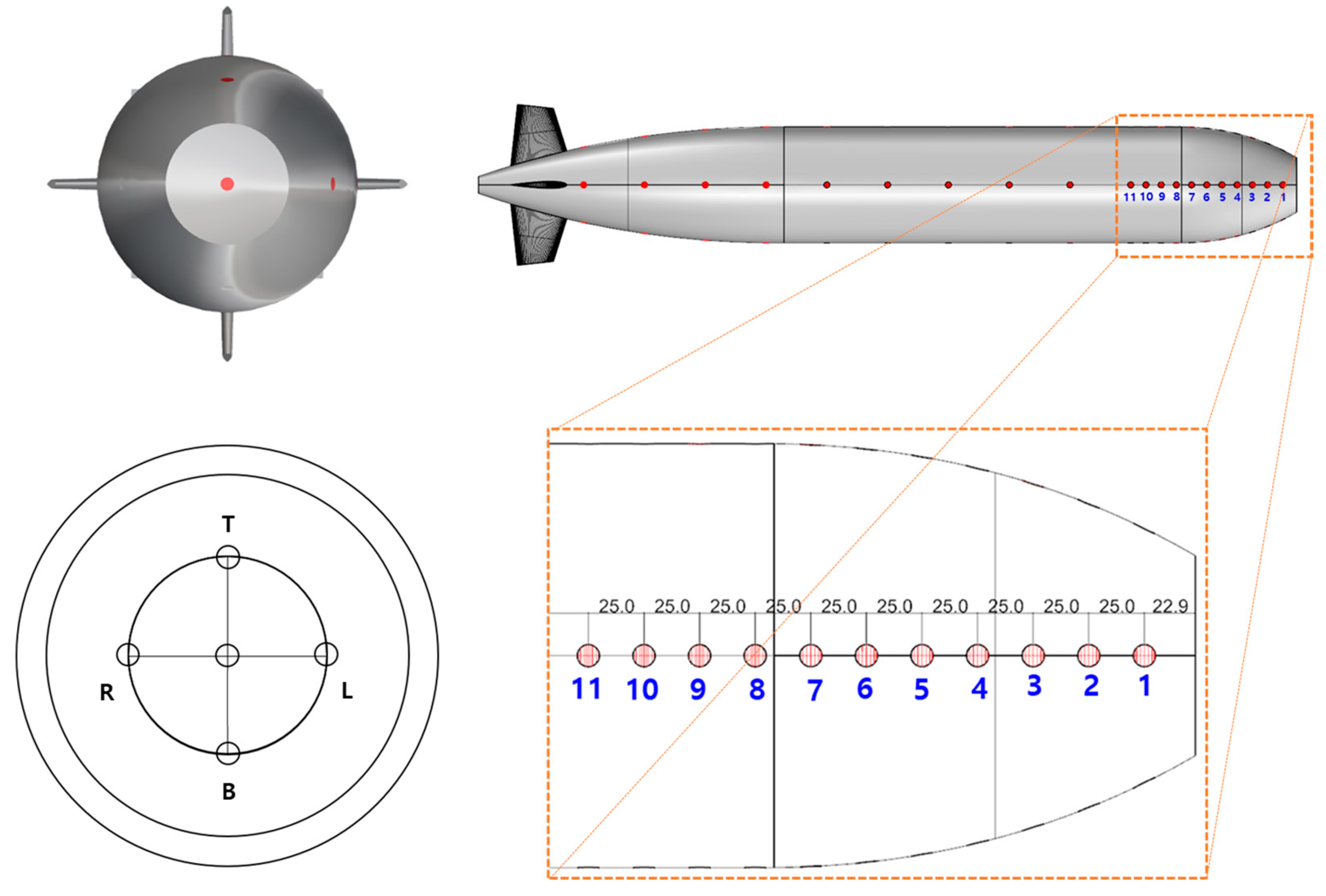
Figure 2.
Coordinate system and motion variables.
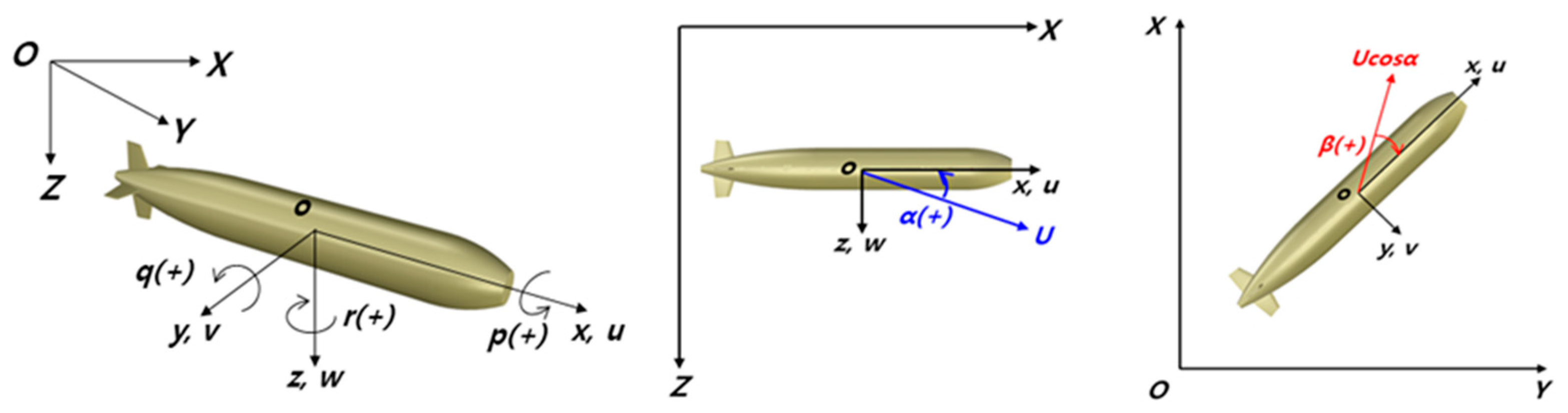
Figure 3.
AUV motion patterns (single).
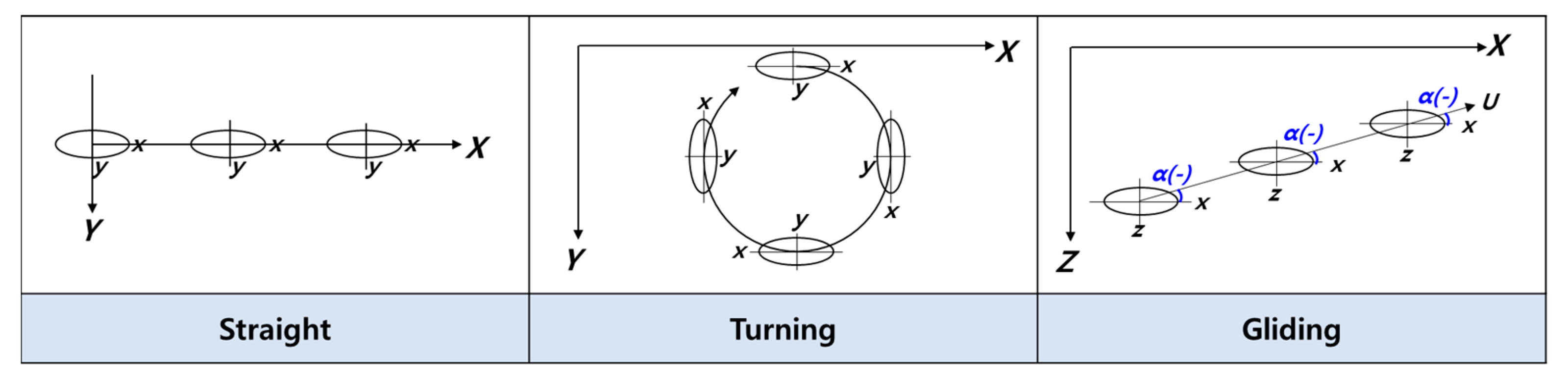
Figure 4.
Flow chart of AUV state estimation.
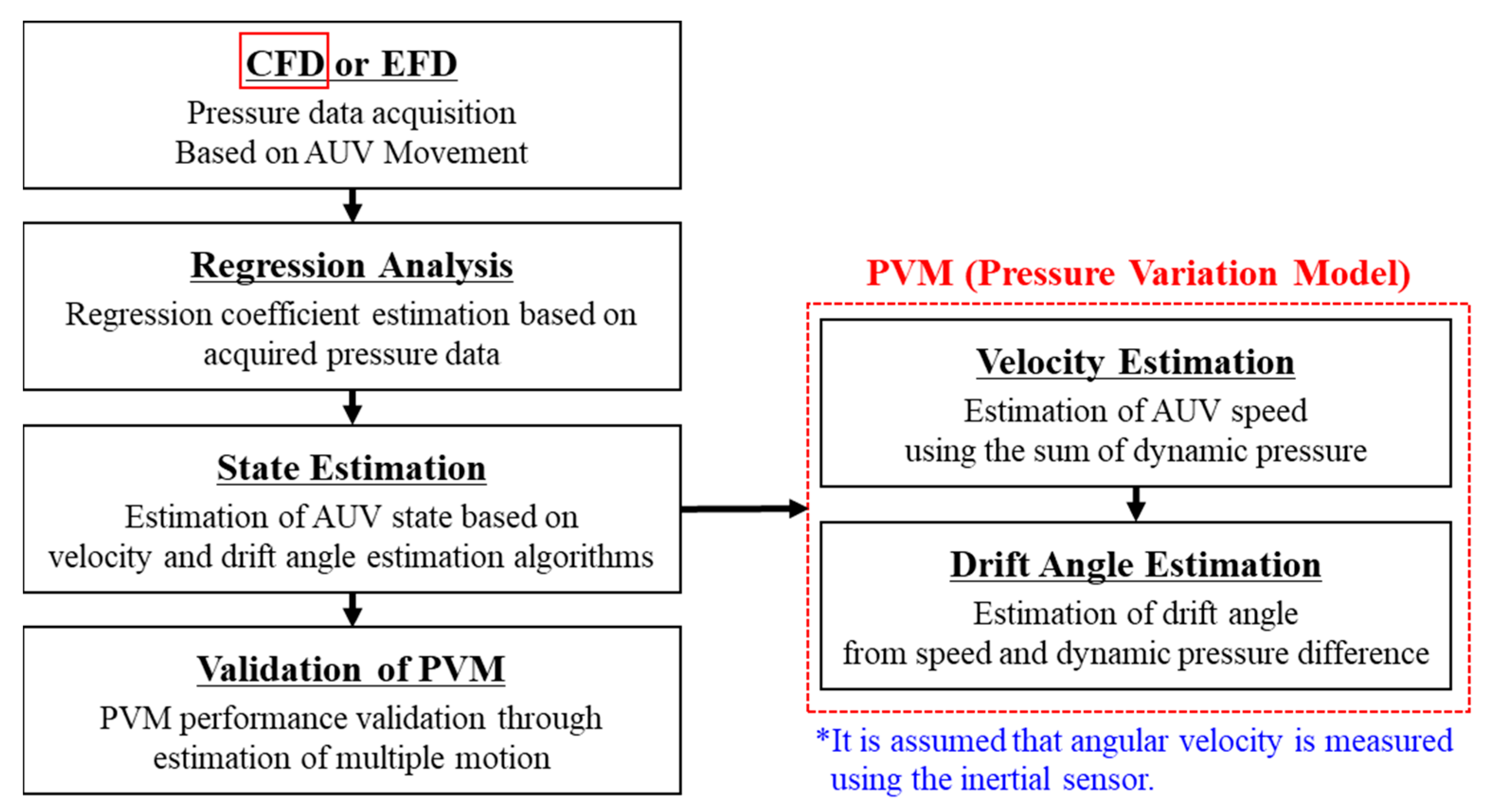
Figure 5.
AUV motion patterns (multiple).
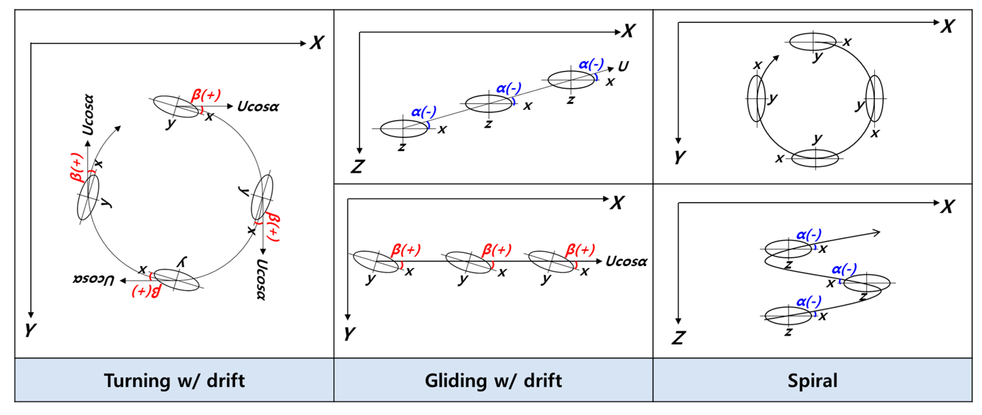
Figure 6.
Numerical simulation domain.
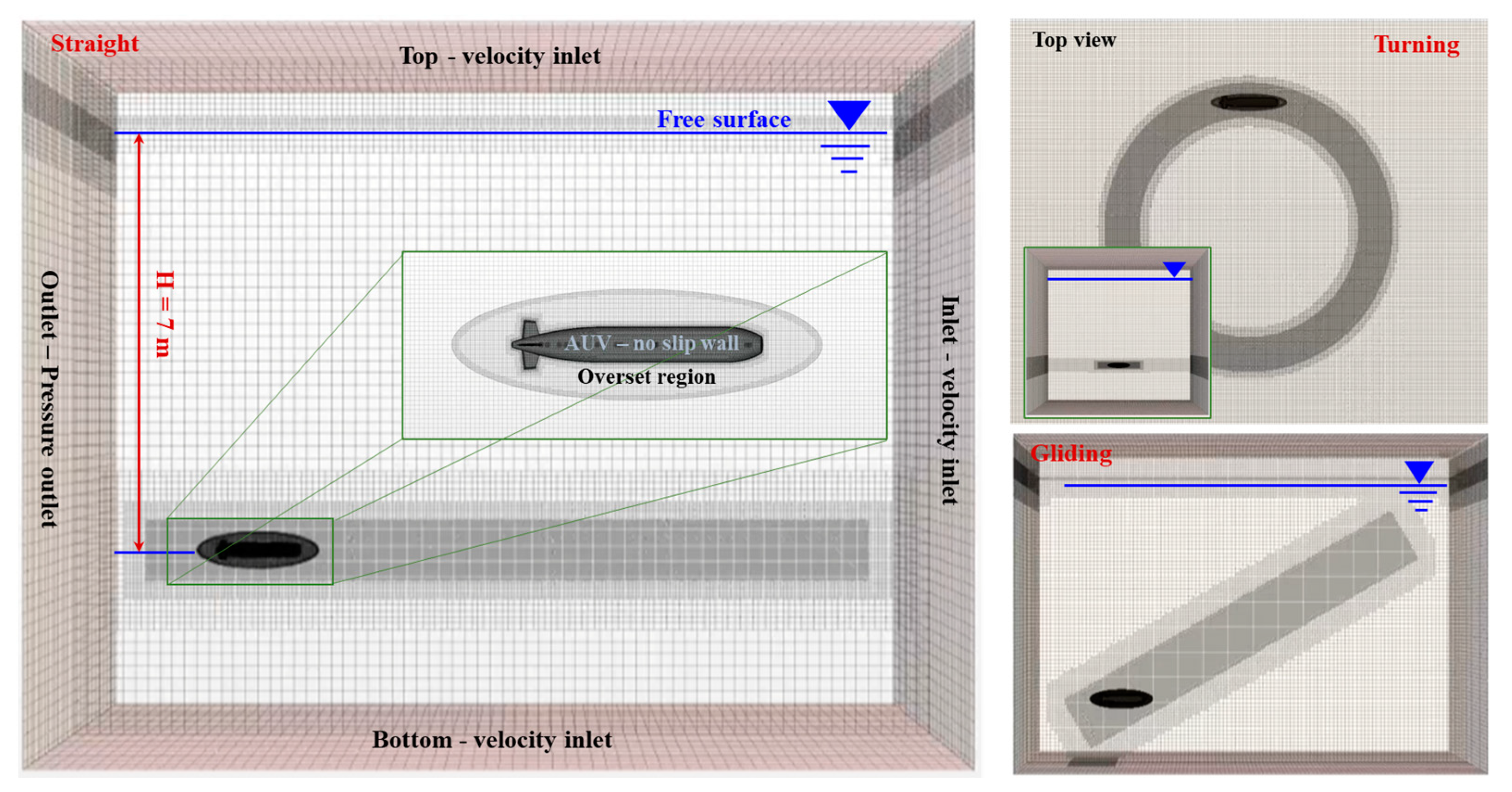
Figure 7.
Pressure on the array of sensors during straight motion.
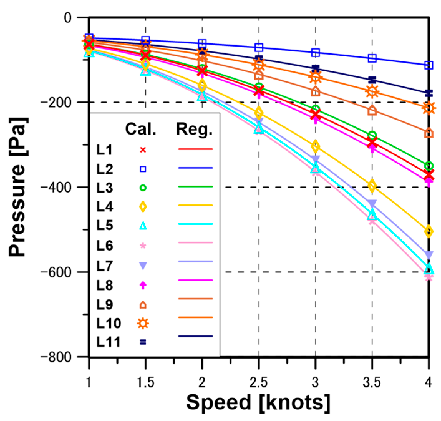
Figure 8.
Pressure on the array of sensors during turning motion.

Table 1.
Geometric details of the test model.
| Length overall [m] | 1.345 |
| Max. diameter [m] | 0.191 |
| Design speed [knots] | 3.0 |
Table 2.
Test conditions.
| Motion | Motion Variable | Note |
|---|---|---|
| Straight | U = 1.0~4.0 [knots] *Interval 0.5 knots | α = 0, β = 0, r = 0, q = 0 |
| Turning | U = 2.0~4.0 [knots] *Interval 1.0 knots r = 0~30 [deg/s] *Interval 5 deg/s | α = 0, β = 0, r ≠ 0, q = 0 |
| Gliding | U = 1.0~4.0 [knots] *Interval 0.5 knots α = 0~−30 [deg] *Interval 5 deg | α ≠ 0, β = 0, r = 0, q = 0 |
Table 3.
The R2 and the MAE for each motion condition and pressure sensor.
| Motion | Sensor | 1 | 2 | 3 | 4 | 5 | 6 | 7 | 8 | 9 | 10 | 11 |
|---|---|---|---|---|---|---|---|---|---|---|---|---|
| Straight (C1, C6) | R2 | 1.00 | 0.99 | 1.00 | 1.00 | 1.00 | 1.00 | 1.00 | 1.00 | 0.99 | 0.99 | 0.99 |
| MAE | 0.24 | 0.24 | 0.28 | 0.27 | 0.25 | 0.23 | 0.21 | 0.38 | 0.42 | 0.42 | 0.42 | |
| Turning (C2, C3) | R2 | 0.93 | 0.94 | 0.95 | 0.90 | 0.74 | 0.70 | 0.84 | 0.94 | 0.94 | 0.94 | 0.94 |
| MAE | 6.62 | 2.34 | 0.27 | 0.33 | 0.32 | 0.30 | 0.26 | 0.24 | 0.37 | 0.39 | 11.48 | |
| Gliding (C4, C5) | R2 | 0.12 | 0.92 | 0.97 | 0.97 | 0.96 | 0.96 | 0.97 | 0.97 | 0.97 | 0.97 | 0.97 |
| MAE | 24.87 | 17.28 | 5.25 | 3.18 | 3.30 | 3.22 | 3.30 | 4.36 | 5.60 | 6.26 | 6.67 |
Table 4.
The R2 and the MAE for each motion condition and pressure sensor.
| Motion | Sensor | 1 | 2 | 3 | 4 | 5 | 6 | 7 | 8 | 9 | 10 | 11 |
|---|---|---|---|---|---|---|---|---|---|---|---|---|
| Gliding (D1, D4) | R2 | 0.93 | 0.99 | 1.00 | 0.99 | 0.97 | 0.96 | 0.94 | 0.97 | 0.98 | 0.97 | 0.97 |
| MAE | 29.42 | 16.00 | 6.05 | 12.05 | 18.91 | 24.77 | 35.44 | 22.39 | 18.21 | 21.29 | 26.42 | |
| Turning (D2, D3) | R2 | 0.98 | 0.99 | 0.99 | 0.99 | 0.98 | 0.94 | 0.52 | 0.64 | 0.20 | 0.84 | 0.94 |
| MAE | 10.03 | 14.62 | 2.37 | 11.14 | 22.04 | 49.06 | 947.1 | 1097 | 1567 | 795.9 | 710.5 |
Table 5.
PVM coefficients.
| Sensor | C1 | C2 | C3 | C4 | C5 | C6 | D1 | D2 | D3 | D4 |
|---|---|---|---|---|---|---|---|---|---|---|
| 1 | −305.1 | −396.1 | −206.1 | −3803.3 | 1976.2 | −174.5 | −1533.5 | −2328.1 | 1947.2 | 145.28 |
| 2 | −64.5 | −364.6 | −2336.0 | −52.7 | −543.6 | −177.0 | −1350.0 | 97.21 | 829.76 | 46.93 |
| 3 | −288.4 | −328.4 | −1701.4 | −510.0 | −34.3 | −179.5 | −1098.3 | 264.52 | 480.09 | −10.02 |
| 4 | −433.6 | −295.8 | −1311.6 | −307.3 | 31.0 | −180.4 | −858.9 | 5.64 | 358.47 | −18.15 |
| 5 | −515.2 | −257.3 | −1119.0 | −209.4 | 36.3 | −180.5 | −656.3 | −79.53 | 248.60 | −21.85 |
| 6 | −535.6 | −232.4 | −1075.2 | −209.8 | 42.2 | −180.1 | −488.2 | −52.10 | 128.54 | −21.81 |
| 7 | −488.6 | −230.2 | −1192.8 | −252.3 | 42.4 | −179.7 | −365.5 | 11.14 | 26.08 | −22.23 |
| 8 | −323.7 | −228.5 | −1522.9 | −254.4 | −6.0 | −183.5 | −325.8 | −36.75 | 29.30 | −13.58 |
| 9 | −212.7 | −236.8 | −1743.7 | −261.3 | −25.1 | −181.9 | −297.3 | −31.41 | 11.47 | 58.43 |
| 10 | −158.8 | −244.4 | −1843.9 | −252.2 | −23.4 | −181.0 | −265.1 | −23.95 | −18.61 | 104.23 |
| 11 | −126.1 | −248.1 | −1900.1 | −20.1 | −229.9 | −180.4 | −240.3 | −24.64 | −41.54 | 144.74 |
Table 6.
Predicted velocities and relative errors for straight motion.
| U | 1.0 | 1.5 | 2.0 | 2.5 | 3.0 | 3.5 | 4.0 |
|---|---|---|---|---|---|---|---|
| Predicted (knots) | 0.991 | 1.498 | 2.002 | 2.504 | 3.004 | 3.498 | 3.999 |
| Relative Err. (%) | −0.944 | −0.109 | 0.098 | 0.163 | 0.118 | −0.048 | −0.016 |
Table 7.
Predicted velocities and relative errors for turning motion.
| U | 2.0 | 3.0 | 4.0 | |||
|---|---|---|---|---|---|---|
| r | Predicted (Knots) | Relative Err. (%) | Predicted (Knots) | Relative Err. (%) | Predicted (Knots) | Relative Err. (%) |
| 0 | 2.004 | 0.176 | 3.005 | 0.179 | 3.999 | 0.035 |
| 5 | 2.001 | 0.049 | 3.007 | 0.223 | 3.997 | 0.087 |
| 10 | 2.012 | 0.606 | 3.015 | 0.499 | 4.017 | 0.417 |
| 15 | 2.001 | 0.046 | 3.022 | 0.737 | 4.010 | 0.262 |
| 20 | 2.001 | 0.034 | 3.000 | −0.006 | 4.015 | 0.377 |
| 25 | 2.016 | 0.297 | 2.994 | −0.200 | 3.984 | −0.400 |
| 30 | 2.045 | 2.241 | 2.995 | −0.170 | 3.978 | −0.544 |
Table 8.
Predicted velocities and relative errors for gliding motion.
| U | 1.0 | 2.0 | 3.0 | 4.0 | ||||
|---|---|---|---|---|---|---|---|---|
| α | Predicted (Knots) | Relative Err. (%) | Predicted (Knots) | Relative Err. (%) | Predicted (Knots) | Relative Err. (%) | Predicted (Knots) | Relative Err. (%) |
| 0 | 0.995 | −0.484 | 2.001 | 0.057 | 3.002 | 0.079 | 4.000 | −0.008 |
| −5 | 1.022 | 2.235 | 2.026 | 1.278 | 3.018 | 0.604 | 4.012 | 0.293 |
| −10 | 1.041 | 4.099 | 2.012 | 0.605 | 2.984 | −0.537 | 3.952 | −1.201 |
| −15 | 1.058 | 5.775 | 1.998 | −0.112 | 2.966 | −1.145 | 3.911 | −2.215 |
| −20 | 1.065 | 6.492 | 2.003 | 0.132 | 2.933 | −2.225 | 3.868 | −3.305 |
| −25 | 1.008 | 0.761 | 1.977 | −1.142 | 2.905 | −3.173 | 3.835 | −4.137 |
| −30 | 0.997 | −0.315 | 2.089 | 4.450 | 3.129 | 4.299 | 4.179 | 4.472 |
Table 9.
Predicted drift angle and relative errors for straight motion ().
| U | 1.0 | 1.5 | 2.0 | 2.5 | 3.0 | 3.5 | 4.0 |
|---|---|---|---|---|---|---|---|
| Predicted | 1.33 | 0.58 | 0.32 | 0.20 | 0.14 | 0.11 | 0.08 |
| Predicted | 1.18 | 0.51 | 0.29 | 0.18 | 0.13 | 0.09 | 0.07 |
Table 10.
Predicted drift angle and relative errors for turning motion ().
| U | 2.0 | 3.0 | 4.0 | |||
|---|---|---|---|---|---|---|
| r | Predicted | Predicted | Predicted | Predicted | Predicted | Predicted |
| 0 | 0.32 | 0.29 | 0.14 | 0.13 | 0.08 | 0.07 |
| 5 | 0.38 | 0.39 | 0.19 | 0.31 | 0.12 | 0.23 |
| 10 | 0.32 | 0.15 | 0.17 | −0.31 | 0.14 | 0.14 |
| 15 | 0.33 | 0.21 | 0.16 | 0.02 | 0.14 | 0.01 |
| 20 | 0.33 | 0.18 | 0.14 | 0.04 | 0.10 | −0.03 |
| 25 | 0.33 | 0.21 | 0.14 | 0.00 | 0.07 | −0.04 |
| 30 | 0.31 | 0.37 | 0.14 | −0.07 | 0.07 | −0.12 |
Table 11.
Predicted drift angle and relative errors for gliding motion ().
| U | 1.0 | 2.0 | 3.0 | 4.0 | ||||
|---|---|---|---|---|---|---|---|---|
| Predicted | Relative Err. (%) | Predicted | Relative Err. (%) | Predicted | Relative Err. (%) | Predicted | Relative Err. (%) | |
| 0 | 1.32 | - | 0.32 | - | 0.14 | - | 0.08 | - |
| −5 | −3.75 | −25.07 | −4.84 | −3.23 | −5.09 | 1.86 | −5.19 | 3.78 |
| −10 | −8.36 | −16.43 | −9.91 | −0.93 | −10.31 | 3.12 | −10.50 | 5.04 |
| −15 | −12.57 | −16.22 | −14.99 | −0.04 | −15.46 | 3.08 | −15.82 | 5.48 |
| −20 | −16.90 | −15.48 | −19.80 | −0.99 | −20.82 | 4.11 | −21.27 | 6.34 |
| −25 | −24.10 | −3.61 | −25.74 | 2.95 | −26.81 | 7.23 | −27.27 | 9.07 |
| −30 | −30.18 | 0.60 | −27.66 | −7.81 | −27.58 | −8.08 | −27.28 | −9.08 |
| U | 1.0 | 2.0 | 3.0 | 4.0 | ||||
| Predicted | ||||||||
| 0 | 1.17 | 0.29 | 0.13 | 0.07 | ||||
| −5 | 1.12 | 0.28 | 0.13 | 0.07 | ||||
| −10 | 1.08 | 0.29 | 0.13 | 0.07 | ||||
| −15 | 1.00 | 0.29 | 0.13 | 0.08 | ||||
| −20 | 1.06 | 0.29 | 0.13 | 0.08 | ||||
| −25 | 1.13 | 0.30 | 0.14 | 0.08 | ||||
| −30 | 1.16 | 0.27 | 0.12 | 0.07 | ||||
Table 12.
Validation conditions.
| Motion | Motion Variable | Note |
|---|---|---|
| Turning w/drift | U = 3.0 [knots] β = 10, 20 [deg] r = 10, 20, 30 [deg/s] | α = 0, β ≠ 0, r ≠ 0, q = 0 |
| Gliding w/drift | U = 1.5, 3.0 [knots] α = −10, −20 [deg] β = 10, 20 [deg] | α ≠ 0, β ≠ 0, r = 0, q = 0 |
| Spiral | U = 3.0 [knots] α = −10, −20, −30 [deg] r = 10, 20, 30 [deg/s] | α ≠ 0, β = 0, r ≠ 0, q = 0 |
Table 13.
Predicted velocities and relative errors for turning with drift motion (U = 3.0 knots, ).
| r | 10 | 20 | 30 | ||||||
|---|---|---|---|---|---|---|---|---|---|
| β | 0 | 10 | 20 | 0 | 10 | 20 | 0 | 10 | 20 |
| Predicted (knots) | 3.004 | 2.960 | 2.681 | 2.994 | 3.059 | 2.934 | 2.996 | 3.182 | 3.116 |
| Relative Err. (%) | 0.119 | 1.354 | 10.64 | 0.196 | 1.947 | 2.204 | 0.134 | 6.071 | 3.865 |
Table 14.
Predicted velocities and relative errors for gliding with drift motion.
| U | 1.5 | 3.0 | ||||||||||
|---|---|---|---|---|---|---|---|---|---|---|---|---|
| α | −10 | −20 | −10 | −20 | ||||||||
| β | 0 | 10 | 20 | 0 | 10 | 20 | 0 | 10 | 20 | 0 | 10 | 20 |
| Predicted (knots) | 1.525 | 1.527 | 1.483 | 1.534 | 1.546 | 1.475 | 2.984 | 3.004 | 2.921 | 2.933 | 2.987 | 2.910 |
| Relative Err. (%) | 1.655 | 1.765 | 1.109 | 2.227 | 3.040 | 1.693 | 0.545 | 0.110 | 2.631 | 2.233 | 0.426 | 3.010 |
Table 15.
Predicted velocities and relative errors for spiral motion (U = 3.0 knots, ).
| α | −10 | −20 | −30 | ||||||
|---|---|---|---|---|---|---|---|---|---|
| r | 10 | 20 | 30 | 10 | 20 | 30 | 10 | 20 | 30 |
| Predicted (knots) | 3.115 | 3.019 | 3.084 | 2.625 | 3.082 | 3.129 | 2.982 | 2.982 | 3.352 |
| Relative Err. (%) | 3.810 | 0.619 | 2.799 | 12.52 | 2.733 | 4.297 | 0.623 | 0.612 | 11.73 |
Table 16.
Predicted drift angle and relative errors for turning with drift motion (U = 3.0 knots, ).
Table 16.
Predicted drift angle and relative errors for turning with drift motion (U = 3.0 knots, ).
| r | 10 | 20 | 30 | |||
|---|---|---|---|---|---|---|
| β | ||||||
| 0 | 0.17 | 0.14 | 0.14 | |||
| 10 | 0.15 | 0.15 | 0.13 | |||
| 20 | 0.19 | 0.16 | 0.14 | |||
| r | 10 | 20 | 30 | |||
| β | Predicted | Relative Err. (%) | Predicted | Relative Err. (%) | Predicted | Relative Err. (%) |
| 0 | −0.32 | - | 0.03 | - | −0.06 | - |
| 10 | 10.83 | 8.29 | 10.21 | 2.07 | 10.34 | 3.44 |
| 20 | 24.79 | 23.93 | 20.70 | 3.50 | 19.41 | −2.94 |
Table 17.
Predicted drift angle and relative errors for gliding with drift motion.
| −10 | ||||||||
| U | 1.5 | 3.0 | ||||||
| Predicted | Relative Err. (%) | Predicted | Relative Err. (%) | Predicted | Relative Err. (%) | Predicted | Relative Err. (%) | |
| 0 | −9.45 | −5.48 | 0.49 | - | −10.31 | 3.12 | 0.13 | - |
| 10 | −8.83 | −11.72 | 10.17 | 1.66 | −9.88 | −1.18 | 10.16 | 1.64 |
| 20 | −9.97 | −0.31 | 22.04 | 10.19 | −10.70 | 7.01 | 22.06 | 10.30 |
| −20 | ||||||||
| U | 1.5 | 3.0 | ||||||
| Predicted | Relative Err. (%) | Predicted | Relative Err. (%) | Predicted | Relative Err. (%) | Predicted | Relative Err. (%) | |
| 0 | −18.85 | −5.73 | 0.49 | - | −20.82 | 4.11 | 0.13 | - |
| 10 | −19.45 | −2.73 | 9.63 | −3.69 | −21.07 | 5.33 | 9.86 | −1.44 |
| 20 | −21.16 | 5.82 | 20.90 | 4.51 | −21.22 | 6.09 | 20.59 | 2.97 |
Table 18.
Predicted drift angle and relative errors for spiral motion (U = 3.0 knots, ).
| −10 | −20 | −30 | ||||
|---|---|---|---|---|---|---|
| r | Predicted | Relative Err. (%) | Predicted | Relative Err. (%) | Predicted | Relative Err. (%) |
| 10 | −10.03 | 0.29 | −28.71 | 43.57 | −33.94 | 13.12 |
| 20 | −9.96 | −0.38 | −20.89 | 4.45 | −33.87 | 12.92 |
| 30 | −9.89 | −1.14 | −20.55 | 2.77 | −26.94 | −10.20 |
| U | −10 | −20 | −30 | |||
| r | Predicted | |||||
| 10 | 0.29 | −0.57 | −0.03 | |||
| 20 | 0.42 | 0.22 | 0.08 | |||
| 30 | 0.69 | 0.43 | 0.91 | |||
Disclaimer/Publisher’s Note: The statements, opinions and data contained in all publications are solely those of the individual author(s) and contributor(s) and not of MDPI and/or the editor(s). MDPI and/or the editor(s) disclaim responsibility for any injury to people or property resulting from any ideas, methods, instructions or products referred to in the content. |
© 2024 by the authors. Licensee MDPI, Basel, Switzerland. This article is an open access article distributed under the terms and conditions of the Creative Commons Attribution (CC BY) license (https://creativecommons.org/licenses/by/4.0/).
Share and Cite
MDPI and ACS Style
Kim, J.-H.; Mai, T.L.; Cho, A.; Heo, N.; Yoon, H.K.; Park, J.-Y.; Byun, S.-H. Establishment of a Pressure Variation Model for the State Estimation of an Underwater Vehicle. Appl. Sci. 2024, 14, 970. https://doi.org/10.3390/app14030970
AMA Style
Kim J-H, Mai TL, Cho A, Heo N, Yoon HK, Park J-Y, Byun S-H. Establishment of a Pressure Variation Model for the State Estimation of an Underwater Vehicle. Applied Sciences. 2024; 14(3):970. https://doi.org/10.3390/app14030970
Chicago/Turabian StyleKim, Ji-Hye, Thi Loan Mai, Aeri Cho, Namug Heo, Hyeon Kyu Yoon, Jin-Yeong Park, and Sung-Hoon Byun. 2024. "Establishment of a Pressure Variation Model for the State Estimation of an Underwater Vehicle" Applied Sciences 14, no. 3: 970. https://doi.org/10.3390/app14030970
Note that from the first issue of 2016, this journal uses article numbers instead of page numbers. See further details here.