
A Helly Model-Based MPC Control System for Jam-Absorption Driving Strategy against Traffic Waves in Mixed Traffic


1
School of Electronics and Control Engineering, Chang’an University, Xi’an 710064, China
2
Department of Built Environment, School of Engineering, Aalto University, P.O. Box 14100, FI-00076 Aalto, Finland
*
Authors to whom correspondence should be addressed.
Appl. Sci. 2024, 14(4), 1424; https://doi.org/10.3390/app14041424
Submission received: 6 January 2024
/
Revised: 2 February 2024
/
Accepted: 3 February 2024
/
Published: 9 February 2024
(This article belongs to the Special Issue Transportation Planning, Management and Optimization)
Abstract
:Traffic waves in traffic flow significantly impact road throughput and fuel consumption and may even lead to severe safety issues. Currently, in connected and autonomous environments, the jam-absorption driving (JAD) strategy shows good performance in dissipating traffic waves. However, the previous JAD strategy has mostly focused on wave dissipation without adequately assessing traffic efficiency and safety. To address this gap, an optimal control problem for JAD in mixed traffic is proposed to reduce traffic waves. The prediction model is developed using the car-following model within a model predictive control (MPC) framework. The Helly model is selected for the manual vehicle. This is because the Helly model is a linear model that describes the car-following phenomenon accurately without delay effect. In addition, the objective function of the prediction model considers both traffic safety and efficiency while satisfying mechanical and safety constraints. Simulation results indicate that the proposed methodology can effectively reduce traffic jams and improve traffic performance on a one-lane freeway. The optimal method is more applicable to complex traffic wave scenarios, providing a new perspective for reducing traffic jams on the freeway.
1. Introduction
Stop-and-go waves are a special traffic phenomenon that is well-known empirically, but it is a little difficult to describe them in traffic models. This is because there are disturbances in the traffic flow that typically arise. Stop-and-go waves are amplified due to the hysteresis effect of the acceleration and deceleration of the vehicle as they propagate upstream [1,2]. Such irregular behavior in traffic flow can cause a series of traffic problems, such as congested traffic, increased fuel consumption, and even a potential safety hazard. Therefore, it is necessary to investigate the problem of traffic wave dissipation.
Many empirical studies have been developed and expanded on how to improve the impact of traffic oscillation on traffic safety and traffic efficiency, and many theories and models have been used to explain the mechanism of traffic oscillation. The key to dissipating stop-and-go waves is to smooth traffic speed on both the temporal and spatial dimensions, by which a stabler and safer flow can be achieved [3]. In the early stage, control approaches using variable speed limits (VSLs) have been proposed, which can smooth the traffic flow speed, optimize the traffic flow, and avoid stop-and-go waves and other unstable states [4,5,6]. One notable example is SPECIALIST [7], using a controlled moving bottleneck to stop-and-go wave dissipation. However, the disturbance cannot be handled due to its feed-forward structure when the VSLs are activated with a demand increment. Some studies developed a model predictive control (MPC) approach of VSLs to resolve jam waves, where the design was based on extended cell transmission models and Eulerian Lighthill–Whitham and Richards (LWR) models [8,9]. However, the performance of VSLs largely relies on the compliance rate and is limited to the installation location and number of variable message signs on the road.
In recent years, with the advent of autonomous driving and communication technology, more precise and emerging control strategies have provided new ideas for improving traffic performance. Some studies have considered vehicle automation and communication systems, and a model-based quadratic programming problem has been developed to minimize traffic congestion [10,11]. Many researchers concluded that cooperative ACC-equipped vehicles can detect and suppress stop-and-go waves [12]. Some researchers have experimentally demonstrated that autonomous vehicle (AV) driving algorithms can be specifically designed to dissipate stop-and-go waves and have created an automated vehicle control strategy called FollowerStopper (FS) [13,14]. Interestingly, the results showed that FS can make the system more uniform, but it cannot increase the average velocity [15]. In connected and autonomous environments, some researchers have proposed a theoretical jam-absorption driving (JAD) strategy to eliminate traffic jams [16] and have derived the theoretical conditions for restricting secondary jams [17]. Additionally, a real-time control system for operating JAD against multiple moving jams was presented on freeway sections [18]. Similarly, some studies have proposed the JAD based on different car-following models to reduce traffic waves and improve traffic performance [19,20,21]. Some studies focus on guiding vehicle trajectories to enhance traffic performance. Taking into account fuel consumption and driving comfort, a piecewise trajectory optimization model was proposed to smooth the platoon of CAVs [22].
MPC has been widely used in traffic control due to its capability of solving multivariable optimization problems, systematically accounting for constraints on both state and control actions, and considering the anticipated future behavior of the system [23]. Recently, some researchers have conducted a review of model predictive path tracking (PT) control for automated road vehicles [24], considering the following MPC methods for PT control: linear MPC [25,26], linear time-varying MPC [27], linear parameter-varying MPC [28], nonlinear MPC [29], hybrid MPC [30], neural network MPC [31], robust MPC [32], and learning MPC [33]. Some researchers have proposed a learning-based model predictive control (LMPC) algorithm for a Formula Student (FS) autonomous vehicle to improve the dynamic model accuracy of the vehicle [34]. Some researchers have summarized the studies on learning-based MPC, focusing on the following three aspects [35]: (1) learning the system dynamics: taking into account the automatic adjustment of the system dynamic model [36], both during operation and between different operational instances; (2) learning the controller design: emphasizing the problem formulation [37,38], such as defining cost functions, constraints, or terminal components, leading to improved closed-loop performance; (3) MPC for safe learning: decoupling the optimization of the objective function subject to constraint conditions [39]. To reduce traffic congestion and improve the safety of bottleneck areas, a dynamic speed control method was proposed using connected and autonomous vehicle (CAV) technology [40]. Based on the model predictive control (MPC) framework and safety potential field (SPF) model, an alternative CAV platoon dynamic control method was developed [41]. Some researchers proposed a multi-objective, guaranteed feasible connected and autonomous vehicle (CAV) platoon control method for signalized isolated intersections with priorities [42]. To capture hybrid traffic flow dynamics, an MPC model embedded with a mixed-integer nonlinear program was developed [43]. To optimize a vehicle platoon system in terms of car-following behavior, a decentralized MPC strategy for longitudinal velocity control was established [44]. Some researchers proposed a comprehensive linear time-varying MPC design for a type of AV to achieve good trajectory tracking in a practical driving scenario [45]. Some researchers proposed a model of predictive control based on ACC to dampen traffic waves and reduce traffic congestion [46,47]. A safety-enhancing eco-driving strategy for CAVs based on a hierarchical distributed framework was proposed to optimize the trajectory of CAVs on a signalized arterial in mixed traffic flow [48]. A polytopic model-based robust predictive control scheme was proposed to construct the path tracking of AVs [49]. For the cooperative control system of CAVs, a distributed control architecture and hierarchical controller based on a multi-agent system (MAS) were proposed to handle complex traffic scenarios [50]. Some researchers have proposed a hierarchical model predictive control framework that can be used for the coordinated and integrated control of a motorway system to achieve traffic flow efficiency, considering that serval vehicles were equipped with specific vehicle automation and communication systems [51].
JAD is a behavior of mitigating traffic jams by dynamically changing the headway of a single vehicle and consists of two actions termed “slow-in” and “fast-out” [52]. The “slow-in” is the action to avoid being captured by a jam and to eliminate it by decelerating and creating a long space headway proactively. The “fast-out” is an action that follows the leading vehicle by quickly accelerating without unnecessary time intervals after the “slow-in”. However, the JAD strategy focused on dissipating traffic waves without evaluating both traffic efficiency and traffic safety fully. To address the gap, this study develops an optimal control problem for JAD against traffic waves, which provides a good trade-off between traffic efficiency and traffic safety. More specifically, the optimal controller is established based on a microscopic car-following model formulated in a model predictive control (MPC) scheme. The objective function of the proposed approach is to minimize acceleration and safety indicators, minimize speed deviation of the last vehicle from the maximum allowable speed, and maximize the total travel distance while satisfying the mechanical and safety constraints.
This paper proceeds as follows: in Section 2, the overall framework is described. Section 3 presents the mathematical formulation, providing explanations for the traffic state dynamics and elaborating on the objective function and system constraints. Section 4 provides numerical design and simulation results. Section 5 presents the conclusions and some topics for future research.
2. The Application Framework
It is well known that the key to JAD strategy is to avoid traffic jams by controlling the headway and velocity of a single vehicle. The mechanism diagram of the JAD strategy is depicted in Figure 1.
The description of the vehicle’s trajectory over some time in Figure 1 is as follows. When the vehicles are in a congested state, absorbing vehicle m decelerates from point A to point B at speed to prevent the traffic wave from propagating upstream, and then the absorbing vehicle m accelerates from point B to point C and travels at free flow speed to eliminate the compression wave caused by a series of actions. Subsequent vehicles follow vehicle m in a car-following behavior. The absorbing vehicle induces a compression wave with speed and an expansion wave with speed arising from A and B, respectively. Eventually, these two waves cancel each other out at point C. Hence, subsequent vehicles at point C run at the initial speed .
To dissipate stop-and-go waves, an MPC scheme is developed based on a car-following model for the JAD strategy. Due to the linearity and intuitiveness of the Helly model, it is chosen for modeling manual vehicles. The MPC is employed to predict the evolution of traffic dynamics through the traffic flow model and compute the optimal control action according to the current state of the system. The schematic view of the overall framework system is depicted in Figure 2. In mixed traffic, connected vehicles use onboard sensors to obtain the position and speed of the vehicle in real time and then transmit the vehicle data back to the traffic management center through the roadside communication system. The processing system analyzes the traffic information to determine if traffic oscillations are occurring on the road. The optimal controller is activated once the phenomenon is detected. In the optimization process, the control input (acceleration) of the system is obtained according to the traffic state of the vehicle and the objective function and constraint conditions. Consequently, vehicles adhere to the advised acceleration for navigation.
3. System Description
Consider a platoon of N (N > 1) heterogeneous vehicles, with each vehicle denoted by an index . Vehicle (i − 1) is the preceding vehicle of vehicle i, for all , and vehicle N is the one in front of vehicle 1. Vehicle N is also referred to as vehicle 0.
3.1. The Manual Vehicle
In the MPC scheme, the Helly model is adopted for the manual vehicle. This decision is based on the fact that the Helly model, being a linear model, can precisely depict the phenomenon of car-following without introducing any delay effects. The Helly model is a simple differential equation, and it is related to the relative distance and speed between two vehicles [53]. To be practically applicable, the model is rewritten by the following equation:
where and are the position and velocity of vehicle i at time step t, the vehicle (i − 1) represents the preceding vehicle of vehicle i. The quantities and are sensitivity parameters; is the desired distance for vehicle i; is the minimum distance between two consecutive vehicles; and is the desired (time) headway.
However, if the gap between vehicles is infinite, the Helly model will cause the continuous acceleration of vehicles and an infinite increase in vehicle speed. Therefore, it is necessary to satisfy the collision-free behavior subjected to safety-related constraints in the traffic dynamics. The string stability of the Helly model is analyzed using Laplace transforms.
By substituting (2) into (1), the formula is as follows:
According to the relative distance and the relative velocity , the expression (3) can be written as:
According to the kinematic law, the following relationships between vehicle position , velocity , and acceleration rate are satisfied:
The derivative of both sides of (3) can be conducted:
The Laplace transform of (6) is represented as:
Using the transfer function, we get
String stability can be guaranteed if and only if [54]. Therefore, the string-stability condition is calculated as:
3.2. Traffic State Dynamics
In a mixed traffic flow environment, it is assumed that the real-time positions and speeds of every vehicle can be obtained. Traffic states of the roadway stretch are represented by the equations of motion at discrete time steps T indexed by k, where (actual) time t = kT. This discrete-time system calls for using constantly accelerated motion law for the interval (k, k + 1] (or (t, t + T]), which is described by
Substituting the discrete-time form of (4) into (10) and (11), the following formulae are derived:
which, using matrix form, results in
In the discrete system, the state vector of vehicle i at time step k is defined as:
where and are the position and speed of vehicle i, respectively. Hence, the matrix (14) can be equivalently rewritten as:
Additionally, and are the following vectors:
and is represented as:
From (5) and (15), we can obtain the following vector form:
In the optimal control scheme, the state–space system model can be formulated as follows:
where the state vector is as depicted in (15), and the control input vector is formed by the acceleration rate and the minimum distance d. Then, can be expressed as:
where N represents the total number of vehicles, m signifies the number of vehicles implementing the JAD strategy, d denotes the minimum distance, and n is the number of human-driven vehicles (HDVs). The state matrix is
where and are given by (17), is a vector for the JAD strategy, and the input matrix is
where is obtained from (18), and is a vector for the JAD strategy. The output matrix is
where represents the minimum time headway from the vehicle in front, and is set to 1 s.
3.3. Objective Function
The objective function of the optimal control problem is constructed as:
In this objective function, the first term represents the minimization of the speed deviation of the last vehicle from the maximum allowable speed over time. It encourages vehicles to maintain an appropriate speed in traffic to ensure safety and efficient driving. The second term is formulated as the minimization of acceleration to guarantee a smoother vehicle trajectory and reduce the fuel consumption for the vehicle traveling. The third term strives to optimize the total travel distance of all vehicles on the roadway. The last term avoids potential rear-end safety risks by introducing safety indicators.
3.4. System Constraints
The constraints are defined to guarantee that vehicle motion complies with the mechanical and safety constraints. Specifically, the vehicle’s speed is not allowed to reverse at any time, and it should also not exceed the maximum speed . The vehicles’ acceleration is bounded between minimum acceleration and maximum acceleration . Thus, the mechanical constraints are formulated as:
To prevent the risk of rear-end collisions between vehicles, the distance between the adjacent vehicles should be greater than or equal to the minimum distance d. Thus, the safety constraint is represented as:
where and are the preceding and following vehicles, respectively. The value of d is related to the vehicles’ length and it is set as 5 m because the length of most vehicles falls between 4 and 4.5 m.
In mixed traffic flow, another safety constraint involves ensuring the satisfaction of the safety threshold metric of the vehicle under speed control, expressed by the time-to-collision (TTC) indicator. TTC serves as a safety performance metric, representing the time required for a rear-end collision risk to occur when the leading and following vehicles maintain their current speeds. Two integrated safety metrics, time-exposed time-to-collision (TET)and time-integrated time-to-collision (TIT), are utilized to evaluate the safety of traffic flow
where l represents the length of the vehicle and l = 4.9 m; t is the time; is the total simulation time; n is the vehicle code; and N is the total number of vehicles. According to the previous literature [55], is set to 2 s.
4. Numerical Simulation
4.1. Experimental Design
To evaluate the effectiveness and practicability of the proposed optimization controller, we conduct the simulation experiment using MATLAB for analysis and modeling. Due to the randomness of the simulation experiment, the experiment is repeated 10 times, and the results are averaged.
A hypothetical single-lane freeway stretch without on-ramps and off-ramps is considered. There are 10 vehicles (20 state vectors) on the road, including the guidance vehicle (CAV, m = 1) and the human-driving vehicle (n = 9). To generate a speed-reduction traffic oscillation, the preceding vehicle decelerates at the maximum comfortable deceleration. After remaining at a low speed for a few seconds, the vehicle accelerates to its maximum speed. According to the previous literature [56], the parameters of the Helly model are set to = 0.7 s−2, = 0.5 s−1, h = 1.2 s. Moreover, the initial minimum distance for vehicles is assumed to be 5 m. The value of the maximum speed is set to 30 m/s. The temporal horizon is 600 s, and the simulation time step is 0.1 s. Additionally, the upper and lower bounds for the acceleration constraint are set to = −3 m/s2 and = 3 m/s2.
4.2. Results and Discussion
To evaluate the effectiveness of the proposed optimal control method, the experiments were tested in scenarios involving both single traffic waves and multiple traffic waves.
4.2.1. The Scenario with a Single Traffic Wave
Given these parameters, a speed-reduction traffic wave was generated. Figure 3 shows the experimental simulation results of the scenario with a single traffic wave, where the black line represents the trajectory from the initial values. The vehicle trajectories and vehicle velocity without control are shown in Figure 3a,b. The vehicle trajectories and speed profiles followed the trajectory of the initial values.
The optimized vehicle trajectories and velocity profiles were compared against those without control, as shown in Figure 3c,d. The trajectories suggested by the optimization model satisfy all constraints in the cost function. By analyzing these profiles, it is observed that the vehicle trajectories and speed profiles became smoother. Moreover, the vehicle velocity was improved within the maximum speed limit, indicating that the optimal control can enhance its fuel economy and traffic efficiency. In Figure 3e, the initial and optimized acceleration profiles are denoted by the blue and red lines, respectively. Based on the acceleration trajectories, it can be observed that optimized acceleration values were relatively small, and they eventually stabilized at zero after 485 s. This demonstrated that JAD optimal control can effectively smooth both high deceleration and acceleration rates, thereby improving the comfort of the human driver.
To better analyze the impact of the optimal control method on traffic congestion, the traffic throughput and safety indicators for different methods were compared in the same scenario. The results of the comparison of performance metrics are reported in Table 1. The results indicated that both the JAD and the proposed optimization control method have improved traffic throughput and reduced the risk of rear-end collisions compared to the no-control case. The performance of the proposed optimal control strategy was superior to that of the previous JAD strategy. Specifically, compared with JAD, the proposed optimization strategy resulted in improvements of 6.05% and 1.66% in the safety indicators TET and TIT and a traffic throughput improvement of 2.65%. This reason is that the cost function of the optimal method, taking into account traffic stability and safety, effectively reduces acceleration. Therefore, the simulation revealed that the proposed optimal control method can effectively dampen traffic waves and improve traffic performance.
4.2.2. The Scenario with Multiple Traffic Waves
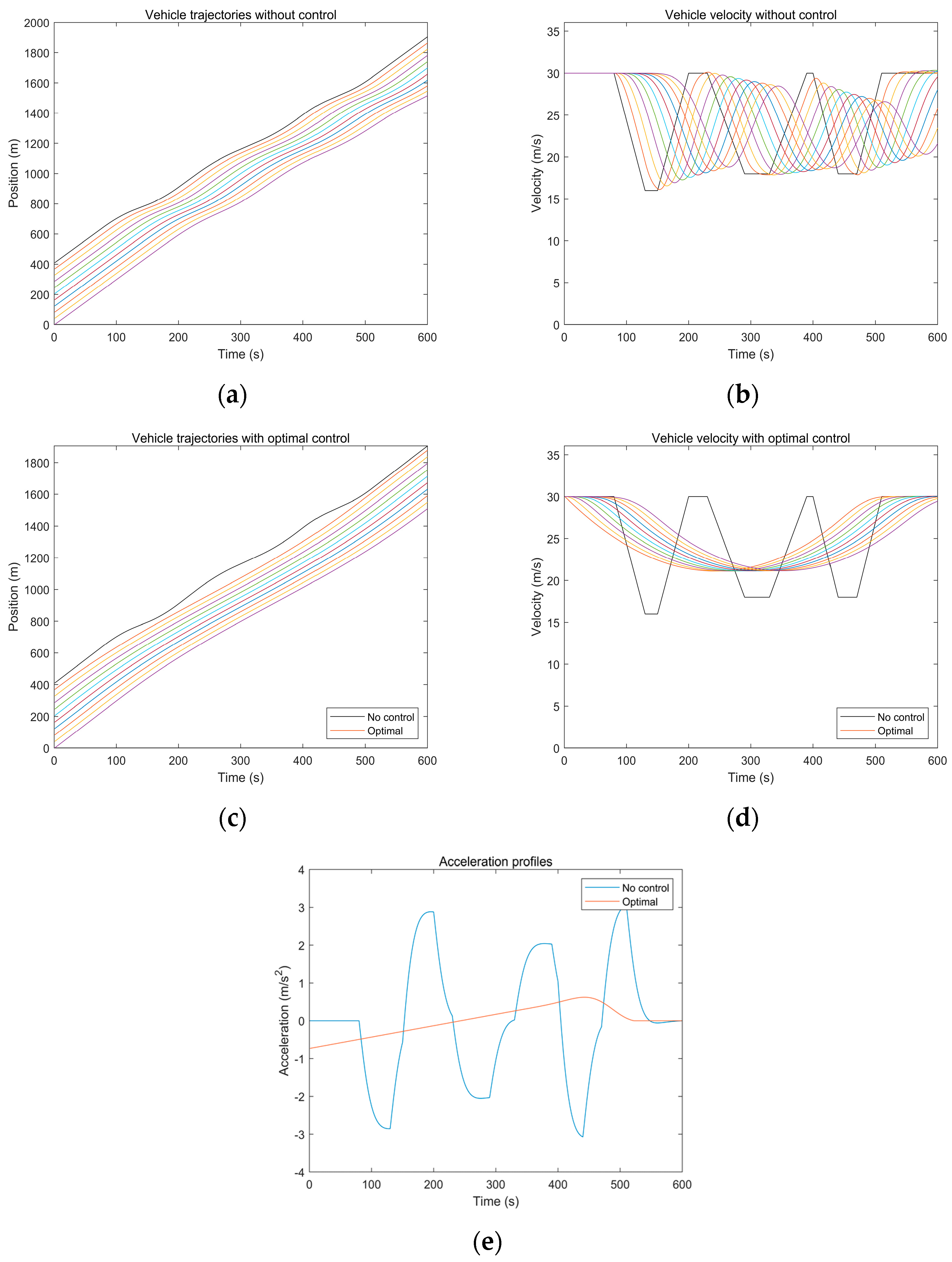
Based on experimental parameters, multiple traffic waves induced by speed were simulated. The results of a scenario with multiple traffic waves are summarized in Figure 4, where the initial trajectory is represented by a black line. In Figure 4a,b, these trajectories without control indicated that the vehicle experienced frequent acceleration and deceleration rates. Similarly, the optimized vehicle and velocity trajectories are shown in Figure 4c,d. The results indicated that, compared to the initial trajectory, the vehicle trajectories tended to become stable after optimizing for smooth speed. According to the constraint conditions, the vehicle velocity was maintained within 30 m/s and exhibited improvement. In Figure 4e, the optimized acceleration trajectory illustrated that the vehicle initially decelerated at a rate of −0.71 m/s2, gradually increased to 0.65 m/s2, and finally tended to be stable and remained at zero after about 570 s. The optimized acceleration became smoother, indicating that the JAD optimal control improved the comfort of the human driver.
The simulation results demonstrated that JAD optimal control within the MPC framework can effectively eliminate traffic oscillations. In addition, the elevation of vehicle speed and the provision of smooth acceleration contribute to an enhancement in fuel economy, traffic efficiency, and the comfort of human drivers. Most importantly, the cost function takes into account the speed difference between the last vehicle and the maximum allowed speed, ensuring the safety of the vehicles.
To demonstrate the feasibility of the proposed optimization control, the change in traffic throughput and traffic safety for the JAD strategy and the optimal control method were quantified in Table 2. It is evident that compared to the JAD strategy, the safety performance indicators of the optimized method showed significant improvement, with a reduction rate of 8.14% in TET and 4.22% in TIT. Simultaneously, there is a notable increase in traffic throughput by 4.25%. The results indicated that the optimal method has better performance in terms of traffic throughput and safety.
Considering the comprehensive analysis above, it can be readily inferred that the proposed optimization control is capable of efficiently mitigating traffic oscillations, enhancing both traffic efficiency and safety, thereby alleviating traffic congestion. It can be found that the performance improvement of the optimized method in the scenario of multiple traffic waves is slightly better than that in the scenario of a single wave. This reveals the proposed method is robust and makes complex traffic flow more stable on a single-lane freeway.
5. Conclusions
To mitigate traffic waves and improve traffic performance, a Helly model-based optimal control problem was developed in mixed flow. This optimal controller takes into account both traffic safety and traffic efficiency. In the MPC scheme, the optimal commands (suitable acceleration values) for all vehicles are calculated to update optimal trajectories, ultimately resulting in a smooth guidance speed. To validate the effectiveness of the proposed methodology, the vehicle trajectories, velocity trajectories, and acceleration trajectories under the optimal method and the no-control case were compared and analyzed. The changes in traffic throughput and safety indicators were computed for different methods (no control, the JAD, and the proposed method). The results showed that the proposed method made the vehicle trajectories and speed trajectories smoother and led to improved speed and reduced acceleration. In terms of performance metrics, the optimization method had better performance compared to the JAD. Interestingly, the performance improvement of the optimal method in the scenario of multiple traffic waves is slightly better than that in the scenario of a single wave. In other words, compared to the no-control case, the proposed method resulted in a 61.48% increase in throughput, a 73.2% reduction in the safety indicator TET, and a 76.21% reduction in the safety indicator TIT. The simulation results demonstrated that the proposed methodology can effectively dampen traffic waves and improve traffic performance, ultimately mitigating traffic congestion and promoting a more stable traffic flow. More importantly, this result suggested that the optimization method is more applicable to complex traffic wave scenarios, which is related to the multi-objective functions. Simultaneously, this experimental simulation in mixed traffic was conducted on a single-lane highway, which holds theoretical significance for alleviating traffic congestion on the freeway.
To simulate real-world traffic conditions more accurately, this work will explore the inclusion of different penetration rates of CAVs, multi-lane configurations, or more intricate traffic scenarios in the future. Lane-changing maneuvers and external disturbances are allowed in experimental tests. Furthermore, alternative car-following models or cost functions will also be investigated to achieve system optimization.
Author Contributions
Conceptualization, C.R.; methodology, H.L.; validation, H.L., C.R. and Y.J. All authors have read and agreed to the published version of the manuscript.
Funding
This work is supported by the Natural Science Basic Research Plan in Shaanxi Province, China (2020JM-255 and 2020JM-238).
Institutional Review Board Statement
Not applicable.
Informed Consent Statement
Not applicable.
Data Availability Statement
Data is contained within the article.
Conflicts of Interest
The authors declare no conflicts of interest.
References
- Li, X.; Cui, J.; An, S.; Parsafard, M. Stop-and-go traffic analysis: Theoretical properties, environmental impacts and oscillation mitigation. Transp. Res. Part B Methodol. 2014, 70, 319–339. [Google Scholar] [CrossRef]
- Zhang, L.; Luan, H.; Zhan, J. Stabilization of stop-and-go waves in vehicle traffic flow. IEEE Trans. Autom. Control 2023, 1–14. [Google Scholar] [CrossRef]
- Ma, J.; Li, X.; Shladover, S.; Rakha, H.A.; Lu, X.Y.; Jagannathan, R.; Dailey, D.J. Freeway speed harmonization. IEEE Trans. Intell. Veh. 2016, 1, 78–89. [Google Scholar] [CrossRef]
- Müller, E.R.; Carlson, R.C.; Kraus, W.; Papageorgiou, M. Microsimulation analysis of practical aspects of traffic control with variable speed limits. IEEE Trans. Intell. Transp. Syst. 2015, 16, 512–523. [Google Scholar] [CrossRef]
- Yang, X.; Lin, Y.; Lu, Y.; Zou, N. Optimal variable speed limit control for real-time freeway congestions. Procedia-Soc. Behav. Sci. 2013, 96, 2362–2372. [Google Scholar] [CrossRef]
- van de Weg, G.S.; Hegyi, A.; Hoogendoorn, S.P.; De Schutter, B. Efficient freeway MPC by parameterization of ALINEA and a speed-limited area. IEEE Trans. Intell. Transp. Syst. 2019, 20, 16–29. [Google Scholar] [CrossRef]
- Hegyi, A.; Hoogendoorn, S.P. Dynamic speed limit control to resolve shock waves on freeways-field test results of the SPECIALIST algorithm. In Proceedings of the 13th International IEEE Conference on Intelligent Transportation Systems, Funchal, Portugal, 19–22 September 2010; pp. 519–524. [Google Scholar] [CrossRef]
- Han, Y.; Hegyi, A.; Yuan, Y.; Hoogendoorn, S.; Papageorgiou, M.; Roncoli, C. Resolving freeway jam waves by discrete first-order model-based predictive control of variable speed limits. Transp. Res. Part C Emerg. Technol. 2017, 77, 405–420. [Google Scholar] [CrossRef]
- Han, Y.; Wang, M.; He, Z.; Li, Z.; Wang, H.; Liu, P. A linear lagrangian model predictive controller of macro-and micro-variable speed limits to eliminate freeway jam waves. Transp. Res. Part C Emerg. Technol. 2021, 128, 103–121. [Google Scholar] [CrossRef]
- Roncoli, C.; Papageorgiou, M.; Papamichail, I. Traffic flow optimisation in presence of vehicle automation and communication systems–part II: Optimal control for multi-lane motorways. Transp. Res. Part C Emerg. Technol. 2015, 57, 260–275. [Google Scholar] [CrossRef]
- Roncoli, C.; Papageorgiou, M.; Papamichail, I. Traffic flow optimisation in presence of vehicle automation and communication systems-Part I: A first-order multi-lane model for motorway traffic. Transp. Res. Part C Emerg. Technol. 2015, 57, 241–259. [Google Scholar] [CrossRef]
- Kim, T.; Jerath, K. Congestion-aware cooperative adaptive cruise control for mitigation of self-organized traffic jams. IEEE Trans. Intell. Transp. Syst. 2021, 23, 6621–6632. [Google Scholar] [CrossRef]
- Stern, R.E.; Cui, S.; Delle Monache, M.L.; Bhadani, R.; Bunting, M.; Churchill, M.; Work, D.B. Dissipation of stop-and-go waves via control of autonomous vehicles: Field experiments. Transp. Res. Part C Emerg. Technol. 2018, 89, 205–221. [Google Scholar] [CrossRef]
- Cummins, L.; Sun, Y.; Reynolds, M. Simulating the effectiveness of wave dissipation by FollowerStopper autonomous vehicles. Transp. Res. Part C Emerg. Technol. 2021, 123, 102954. [Google Scholar] [CrossRef]
- Nateeboon, T.; Tawabutr, H.; Termsaithong, T.; Hirunsirisawat, E. Ability to damp traffic wave when controlling every car on the road by FollowerStopper controller. In Proceedings of the Journal of Physics: Conference Series, Siam Physics Congress 2018 (SPC2018), Pitsanulok, Thailand, 21–23 May 2018; Volume 1144. [Google Scholar] [CrossRef]
- Nishi, R.; Tomoeda, A.; Shimura, K.; Nishinari, K. Theory of jam-absorption driving. Transp. Res. Part B Methodol. 2013, 50, 116–129. [Google Scholar] [CrossRef]
- Nishi, R. Theoretical conditions for restricting secondary jams in jam-absorption driving scenarios. Phys. A Stat. Mech. Its Appl. 2020, 542, 123393. [Google Scholar] [CrossRef]
- Li, S.; Yanagisawa, D.; Nishinari, K. A jam-absorption driving system for reducing multiple moving jams by estimating moving jam propagation. Transp. Res. Part C Emerg. Technol. 2024, 158, 104394. [Google Scholar] [CrossRef]
- Taniguchi, Y.; Nishi, R.; Ezaki, T.; Nishinari, K. Jam-absorption driving with a car-following model. Phys. A Stat. Mech. Its Appl. 2015, 433, 304–315. [Google Scholar] [CrossRef]
- He, Z.; Zheng, L.; Song, L.; Zhu, N. A jam-absorption driving strategy for mitigating traffic oscillations. IEEE Trans. Intell. Transp. Syst. 2016, 18, 802–813. [Google Scholar] [CrossRef]
- Zheng, Y.; Zhang, G.; Li, Y.; Li, Z. Optimal jam-absorption driving strategy for mitigating rear-end collision risks with os-cillations on freeway straight segments. Accid. Anal. Prev. 2020, 135, 105367. [Google Scholar] [CrossRef]
- Li, X.; Ghiasi, A.; Xu, Z.; Qu, X. A piecewise trajectory optimization model for connected automated vehicles: Exact optimization algorithm and queue propagation analysis. Transp. Res. Part B Methodol. 2018, 118, 429–456. [Google Scholar] [CrossRef]
- Salzmann, T.; Kaufmann, E.; Arrizabalaga, J.; Pavone, M.; Scaramuzza, D.; Ryll, M. Real-time neural MPC: Deep learning model predictive control for quadrotors and agile robotic platforms. IEEE Robot. Autom. Lett. 2023, 8, 2397–2404. [Google Scholar] [CrossRef]
- Stano, P.; Montanaro, U.; Tavernini, D.; Tufo, M.; Fiengo, G.; Novella, L.; Sorniotti, A. Model predictive path tracking control for automated road vehicles: A review. Annu. Rev. Control 2023, 55, 194–236. [Google Scholar] [CrossRef]
- Ghandriz, T.; Jacobson, B.; Nilsson, P.; Laine, L. Trajectory-following and off-tracking minimisation of long combination vehicles: A comparison between nonlinear and linear model predictive control. Veh. Syst. Dyn. 2024, 62, 277–310. [Google Scholar] [CrossRef]
- Cao, J.; Song, C.; Peng, S.; Song, S.; Zhang, X.; Xiao, F. Trajectory tracking control algorithm for autonomous vehicle considering cornering characteristics. IEEE Access 2020, 8, 59470–59484. [Google Scholar] [CrossRef]
- Ahn, T.; Lee, Y.; Park, K. Design of integrated autonomous driving control system that incorporates chassis controllers for improving path tracking performance and vehicle stability. Electronics 2021, 10, 144. [Google Scholar] [CrossRef]
- Liang, Y.; Li, Y.; Khajepour, A.; Zheng, L. Multi-model adaptive predictive control for path following of autonomous vehicles. IET Intell. Transp. Syst. 2020, 14, 2092–2101. [Google Scholar] [CrossRef]
- Chowdhri, N.; Ferranti, L.; Iribarren, F.S.; Shyrokau, B. Integrated nonlinear model predictive control for automated driving. Control Eng. Pract. 2021, 106, 104654. [Google Scholar] [CrossRef]
- Zhang, K.; Sprinkle, J.; Sanfelice, R.G. Computationally aware control of autonomous vehicles: A hybrid model predictive control approach. Auton. Robot. 2015, 39, 503–517. [Google Scholar] [CrossRef]
- Spielberg, N.A.; Brown, M.; Gerdes, J.C. Neural network model predictive motion control applied to automated driving with unknown friction. IEEE Trans. Control Syst. Technol. 2021, 30, 1934–1945. [Google Scholar] [CrossRef]
- Hang, P.; Xia, X.; Chen, G.; Chen, X. Active safety control of automated electric vehicles at driving limits: A tube-based MPC approach. IEEE Trans. Transp. Electrif. 2021, 8, 1338–1349. [Google Scholar] [CrossRef]
- Karimshoushtari, M.; Novara, C.; Tango, F. How imitation learning and human factors can be combined in a model predictive control algorithm for adaptive motion planning and control. Sensors 2021, 21, 4012. [Google Scholar] [CrossRef]
- Costa, G.; Pinho, J.; Botto, M.A.; Lima, P.U. Online learning of MPC for autonomous racing. Robot. Auton. Syst. 2023, 167, 104469. [Google Scholar] [CrossRef]
- Hewing, L.; Wabersich, K.P.; Menner, M.; Zeilinger, M.N. Learning-based model predictive control: Toward safe learning in control. Annu. Rev. Control Robot. Auton. Syst. 2020, 3, 269–296. [Google Scholar] [CrossRef]
- Adetola, V.; Guay, M. Robust adaptive MPC for constrained uncertain nonlinear systems. Int. J. Adapt. Control Signal Process. 2011, 25, 155–167. [Google Scholar] [CrossRef]
- Borrelli, F.; Bemporad, A.; Morari, M. Predictive Control for Linear and Hybrid Systems, 1st ed.; Cambridge University Press: New York, NY, USA, 2017; pp. 9–448. [Google Scholar] [CrossRef]
- Jiang, S.; Keyvan-Ekbatani, M. Hybrid perimeter control with real-time partitions in heterogeneous urban networks: An integration of deep learning and MPC. Transp. Res. Part C Emerg. Technol. 2023, 154, 104240. [Google Scholar] [CrossRef]
- Stoffel, P.; Henkel, P.; Rätz, M.; Kümpel, A.; Müller, D. Safe operation of online learning data driven model predictive control of building energy systems. Energy AI 2023, 14, 100296. [Google Scholar] [CrossRef]
- Ding, H.; Zhang, L.; Chen, J.; Zheng, X.; Pan, H.; Zhang, W. MPC-based dynamic speed control of CAVs in multiple sections upstream of the bottleneck area within a mixed vehicular environment. Phys. A Stat. Mech. Its Appl. 2023, 613, 128542. [Google Scholar] [CrossRef]
- Li, L.; Gan, J.; Qu, X.; Lu, W.; Mao, P.; Ran, B. A dynamic control method for CAVs platoon based on the MPC framework and safety potential field model. KSCE J. Civ. Eng. 2021, 25, 1874–1886. [Google Scholar] [CrossRef]
- Wang, C.; Dai, Y.; Xia, J. A CAV platoon control method for isolated intersections: Guaranteed feasible multi-objective approach with priority. Energies 2020, 13, 625. [Google Scholar] [CrossRef]
- Qiu, J.; Du, L. Cooperative trajectory control for synchronizing the movement of two connected and autonomous vehicles separated in a mixed traffic flow. Transp. Res. Part B Methodol. 2023, 174, 102769. [Google Scholar] [CrossRef]
- Wen, J.; Wang, S.; Wu, C.; Xiao, X.; Lyu, N. A longitudinal velocity CF-MPC model for connected and automated vehicle platooning. IEEE Trans. Intell. Transp. Syst. 2022, 24, 6463–6476. [Google Scholar] [CrossRef]
- Pang, H.; Liu, N.; Hu, C.; Xu, Z. A practical trajectory tracking control of autonomous vehicles using linear time-varying MPC method. Proc. Inst. Mech. Eng. Part D J. Automob. Eng. 2022, 236, 709–723. [Google Scholar] [CrossRef]
- Zhou, H.; Zhou, A.; Li, T.; Chen, D.; Peeta, S.; Laval, J. Congestion-mitigating MPC design for adaptive cruise control based on Newell’s car following model: History outperforms prediction. Transp. Res. Part C Emerg. Technol. 2022, 142, 103801. [Google Scholar] [CrossRef]
- Wang, J.; Lian, Y.; Jiang, Y.; Xu, Q.; Li, K.; Jones, C.N. Distributed data-driven predictive control for cooperatively smoothing mixed traffic flow. Transp. Res. Part C Emerg. Technol. 2023, 155, 104274. [Google Scholar] [CrossRef]
- Zhou, Q.; Zhou, B.; Hu, S.; Roncoli, C.; Wang, Y.; Hu, J.; Lu, G. A safety-enhanced eco-driving strategy for connected and autonomous vehicles: A hierarchical and distributed framework. Transp. Res. Part C Emerg. Technol. 2023, 156, 104320. [Google Scholar] [CrossRef]
- Liang, J.; Tian, Q.; Feng, J.; Pi, D.; Yin, G. A polytopic model-based robust predictive control scheme for path tracking of autonomous vehicles. IEEE Trans. Intell. Veh. 2023, 1–11. [Google Scholar] [CrossRef]
- Liang, J.; Li, Y.; Yin, G.; Xu, L.; Lu, Y.; Feng, J.; Shen, T.; Cai, G. A MAS-based hierarchical architecture for the cooperation control of connected and automated vehicles. IEEE Trans. Veh. Technol. 2022, 72, 1559–1573. [Google Scholar] [CrossRef]
- Roncoli, C.; Papamichail, I.; Papageorgiou, M. Hierarchical model predictive control for multi-lane motorways in presence of vehicle automation and communication systems. Transp. Res. Part C Emerg. Technol. 2016, 62, 117–132. [Google Scholar] [CrossRef]
- Nishi, R.; Watanabe, T. System-size dependence of a jam-absorption driving strategy to remove traffic jam caused by a sag under the presence of traffic instability. Phys. A Stat. Mech. Its Appl. 2022, 600, 127512. [Google Scholar] [CrossRef]
- Helly, W. Simulation of bottlenecks in single lane traffic flow. In Proceedings of the Theory of Traffic Flow Symposium, Warren, MI, USA, 7–8 December 1959. [Google Scholar]
- Mattas, K.; Albano, G.; Donà, R.; He, Y.; Ciuffo, B. On the relationship between traffic hysteresis and string stability of vehicle platoons. Transp. Res. Part B Methodol. 2023, 174, 102785. [Google Scholar] [CrossRef]
- Das, S.; Maurya, A.K. Defining Time-to-Collision thresholds by the type of lead vehicle in non-lane-based traffic environments. IEEE Trans. Intell. Transp. Syst. 2020, 21, 4972–4982. [Google Scholar] [CrossRef]
- Rosas-Jaimes, O.A.; Quezada-Téllez, L.A.; Fernández-Anaya, G. Control designs and stability analyses for Helly’s car-following model. Int. J. Mod. Phys. C 2018, 29, 1850025. [Google Scholar] [CrossRef]
Figure 1.
The schematic diagram of the jam-absorption driving (JAD) strategy.
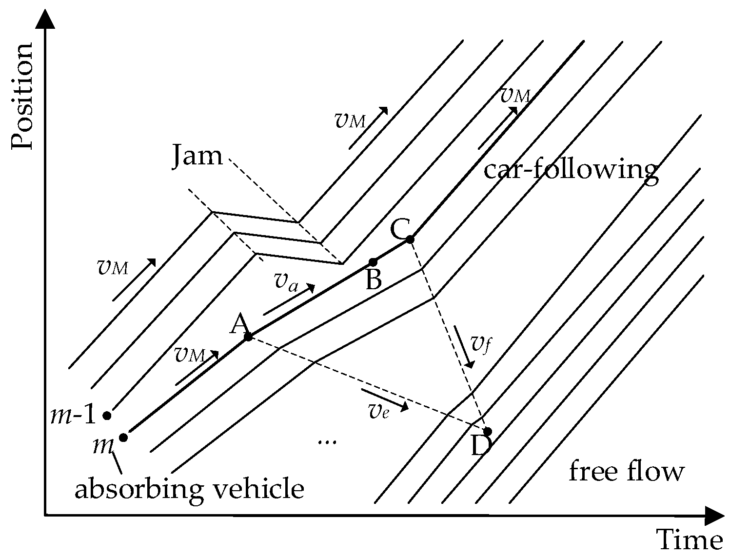
Figure 2.
The schematic view of the overall framework.
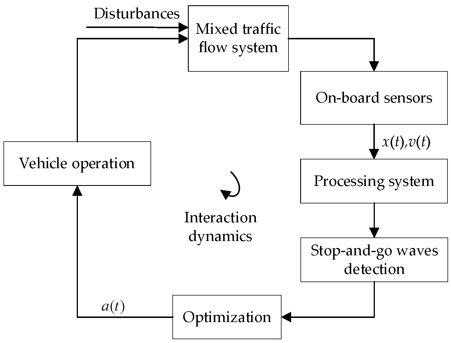
Figure 3.
The results of the scenario with a single stop-and-go wave: (a) The vehicle trajectories without control; (b) The velocity trajectories without control; (c) The optimized vehicle trajectories; (d) The optimized velocity trajectories; (e) The acceleration profiles. (The black line represents the initial trajectory without control for (a–d). For (e), the blue and red lines correspond to the initial and optimized acceleration profiles, respectively).
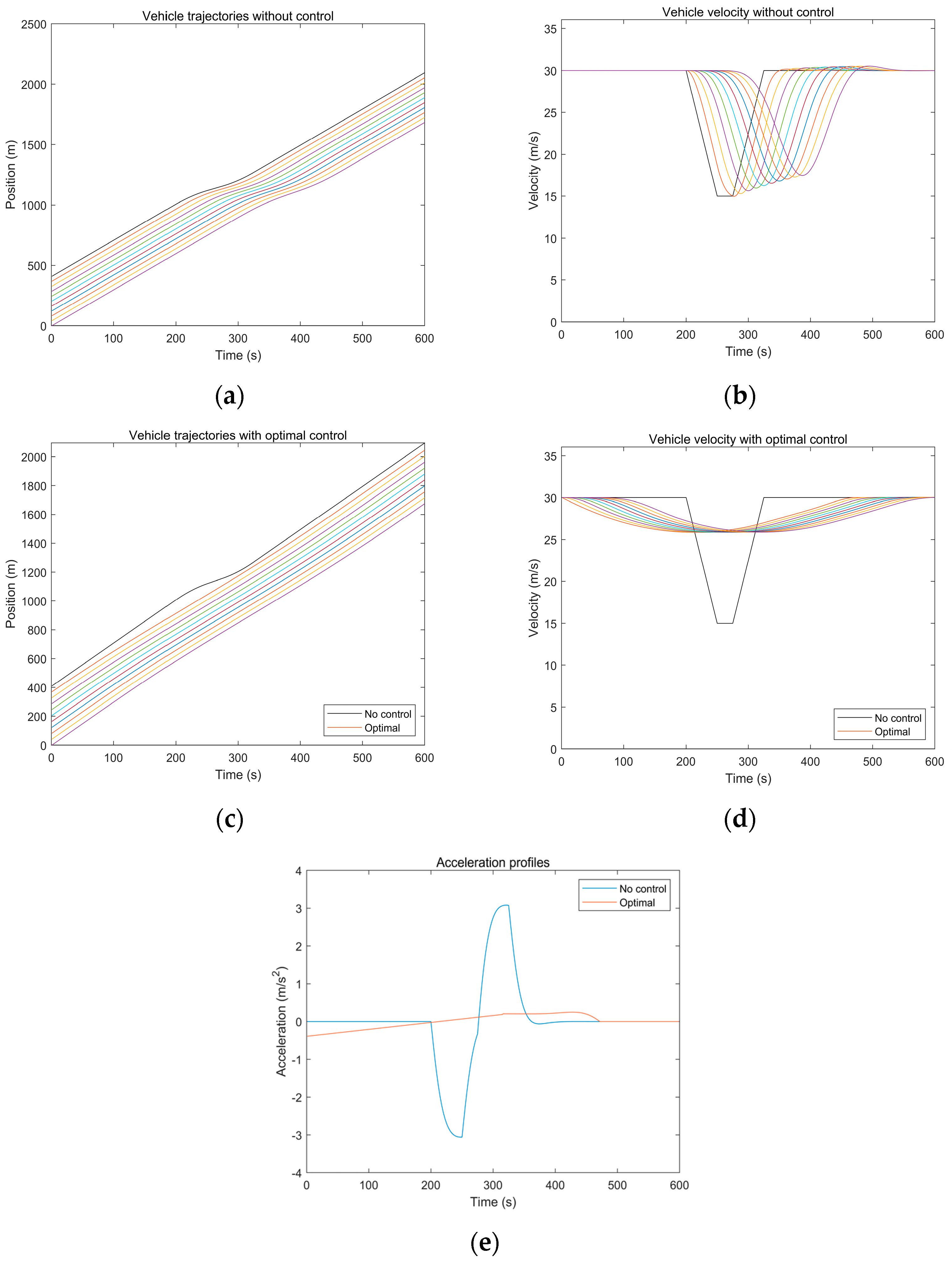
Figure 4.
The results of a scenario with multiple stop-and-go waves: (a) The vehicle trajectories without control; (b) The velocity trajectories without control; (c) The optimized vehicle trajectories; (d) The optimized velocity trajectories; (e) The acceleration profiles. (The black line represents the initial trajectory without control for (a–d). For (e), the blue and red lines correspond to the initial and optimized acceleration profiles, respectively).

Table 1.
Comparison of performance metrics for different methods in the scenario of a single stop-and-go wave.
Table 1.
Comparison of performance metrics for different methods in the scenario of a single stop-and-go wave.
| Methods | The Change in Performance Metrics (%) | ||
|---|---|---|---|
| Throughput | TET | TIT | |
| No control | 0 | 0 | 0 |
| JAD | 58.46 | −65.96 | −73.65 |
| Optimal control | 61.11 | −72.01 | −75.31 |
Table 2.
Comparison of performance metrics for different strategies.
| Methods | The Change in Performance Metrics (%) | ||
|---|---|---|---|
| Throughput | TET | TIT | |
| No control | 0 | 0 | 0 |
| JAD | 57.23 | −65.06 | −71.99 |
| Optimal control | 61.48 | −73.20 | −76.21 |
Disclaimer/Publisher’s Note: The statements, opinions and data contained in all publications are solely those of the individual author(s) and contributor(s) and not of MDPI and/or the editor(s). MDPI and/or the editor(s) disclaim responsibility for any injury to people or property resulting from any ideas, methods, instructions or products referred to in the content. |
© 2024 by the authors. Licensee MDPI, Basel, Switzerland. This article is an open access article distributed under the terms and conditions of the Creative Commons Attribution (CC BY) license (https://creativecommons.org/licenses/by/4.0/).
Share and Cite
MDPI and ACS Style
Li, H.; Roncoli, C.; Ju, Y. A Helly Model-Based MPC Control System for Jam-Absorption Driving Strategy against Traffic Waves in Mixed Traffic. Appl. Sci. 2024, 14, 1424. https://doi.org/10.3390/app14041424
AMA Style
Li H, Roncoli C, Ju Y. A Helly Model-Based MPC Control System for Jam-Absorption Driving Strategy against Traffic Waves in Mixed Traffic. Applied Sciences. 2024; 14(4):1424. https://doi.org/10.3390/app14041424
Chicago/Turabian StyleLi, Haizhen, Claudio Roncoli, and Yongfeng Ju. 2024. "A Helly Model-Based MPC Control System for Jam-Absorption Driving Strategy against Traffic Waves in Mixed Traffic" Applied Sciences 14, no. 4: 1424. https://doi.org/10.3390/app14041424
Note that from the first issue of 2016, this journal uses article numbers instead of page numbers. See further details here.