Frequency-Dependent Contrast Enhancement for Conductive and Non-Conductive Materials in Electrical Impedance Tomography

Abstract

This research investigates the critical role of frequency selection in Electrical Impedance Tomography (EIT), a non-invasive imaging technique that reconstructs internal conductivity distributions through injected electrical currents. Empirical frequency selection is paramount to maximizing the fidelity and specificity of EIT images. The study explores the impact of distinct frequency ranges—low, medium, and high—on image contrast and clarity, particularly focusing on differentiating conductive materials from non-conductive materials. The findings reveal distinct empirical frequency bands for enhancing the respective contrasts: 15–38 kHz for conductive materials (copper) and 45–75 kHz for non-conductive materials (acrylic resin). These insights shed light on the frequency-dependent nature of material contrast in EIT images, guiding the selection of empirical operating ranges for various target materials. This research paves the way for improved sensitivity and broader applicability of EIT in diverse areas.

1. Introduction

Electrical Impedance Tomography (EIT) is a non-destructive testing or non-invasive imaging modality that uses electrical currents to delineate impedance, the resistance to electric currents, within a body or object. In various scientific and medical fields, EIT has become an indispensable tool that provides deep insight into material structures. EIT is used in a variety of applications in life, medicine, and industry, typically in the following:

• Lung imaging: EIT plays a crucial role in the monitoring of lung ventilation and perfusion in real-time, contributing significantly to critical care and lung studies [1].
• Breast imaging: The ability of EIT to distinguish between normal and malignant breast tissues based on impedance contrast shows promise in advancing early breast cancer diagnosis [2].
• Brain function monitoring: Changes in brain impedance, reflecting neuronal activity or blood flow, position EIT as a valuable tool to observe brain functions [3].
• Soil moisture measurement: In agriculture and environmental science, EIT helps estimate soil moisture and salinity levels [4].
• Oil reservoir characterization: The oil and gas industry uses EIT to visualize the distribution of oil, water, and gas in porous rocks, helping to analyze reservoirs [5].

The capability of EIT to reconstruct images based on an object’s impedance distribution poses unique challenges and opportunities, particularly in differentiating materials with distinct electrical properties. Conductive materials, such as metals, saline solutions, or blood, permit the easy passage of electric currents, whereas non-conductive materials, such as plastics, resins, or air, resist electric currents.

The frequency of the applied electric current is pivotal in determining how materials exhibit conductive or non-conductive characteristics. Spanning across the electromagnetic spectrum, from radio waves to gamma rays, frequency influences material responses, giving rise to the concept of frequency-dependent impedance. Impedance spectroscopy, used to understand these responses, provides insight into the structure and function of materials.

Previous research has focused mainly on post-reconstruction contrast enhancement using techniques such as quantitative phase imaging, multi-frequency approaches, diverse reconstruction algorithms, and artificial intelligence (machine learning and deep learning) [6,7,8,9,10,11,12,13,14,15]. An often overlooked consideration is determining the appropriate frequency range for each type of material to enhance the initial contrast. This study addresses this gap by establishing an empirical frequency range for both conductive and non-conductive materials through systematic experiments and evaluation indices, to provide valuable references for enhancing contrast.

The experimental design includes a comprehensive investigation of the frequency-dependent contrast behavior in EIT. The process carried out a series of experiments with different materials, such as copper and acrylic resin, in various environments and configurations. The range of frequencies explored in these experiments was deliberately varied to observe how the contrast between materials changed with different excitation frequencies.

The decision of what constitutes an “empirical” frequency range was based on a combination of analytical indices, including contrast, sharpness, and contrast-to-noise ratio (CNR). These indices were calculated from the reconstructed conductivity images obtained during the experiments. The goal was to identify frequency ranges in which these indices demonstrated favorable values, indicating enhanced contrast, resolution, and clarity in the EIT images. This study aimed to empirically determine frequency ranges that consistently provide desirable imaging outcomes across multiple experiments and conditions. This pragmatic approach aligns with the experimental nature of the study and the goal of providing practical insights into frequency-dependent contrast enhancement in EIT.

The study delves into how different frequencies impact the contrast of conductive metals and non-conductive plastics in EIT images, employing principles from electromagnetic theory and impedance spectroscopy. The study objectives encompass:

• Determining low-, medium-, and high-frequency ranges that enhance or diminish the contrast of metals and plastics in EIT images.
• Understanding the contrast enhancement mechanism: exploring how frequency selection can maximize the contrast between metals and plastics.
• Expanding EIT imaging techniques: providing insights for selective imaging to broaden the applications of EIT.

The paper will cover the methodology, experimental setup, results, and discussion, concluding with potential directions for future research in this dynamically evolving field.

2. Materials and Methods

2.1. Material Preparation and Properties

Frequency-dependent contrast enhancement in EIT involves complex interactions between electromagnetic fields and materials, mainly guided by the frequency-dependent electrical properties of the substances under examination [16,17]. The crucial electrical parameters in this context are conductivity and permittivity, which exhibit varying behaviors in response to the frequency of the applied electrical signal. Within specific frequency ranges, materials may display distinct responses to the electric field, leading to increased contrast in EIT images. This phenomenon is elucidated through materials’ polarization and relaxation processes [18,19]. At lower frequencies, the electric field induces polarization, aligning charged particles within the material. This alignment contributes to alterations in the material’s electrical properties, consequently influencing impedance measurements. By contrast, at higher frequencies, relaxation processes occur as the material’s charges respond to the rapidly changing electric field. The intricate interplay between these mechanisms, along with the inherent electrical characteristics of the materials, collectively shapes the observed contrast in EIT images.

Furthermore, the influence of frequency on the distribution of charges within materials can induce variations in impedance, which the EIT system can delicately detect. Materials with distinct electrical properties, such as conductive and non-conductive substances, may exhibit different responses to different frequencies, highlighting their contrasts [20]. Understanding this frequency-dependent behavior is essential for fine-tuning imaging parameters, as specific frequency ranges can accentuate impedance differences between materials, resulting in clearer and more pronounced contrasts in EIT images. Essentially, the enhancement of contrast in EIT, dependent on frequency, reflects the intricate relationship between the frequency-dependent electrical properties of materials and the sensitivity of the EIT system to these variations. Delving into the specifics of this mechanism entails considering the molecular and atomic responses of materials to the applied electric field across a spectrum of frequencies, laying the groundwork for interpreting and optimizing contrast in EIT imaging.

Copper, renowned for its electrical conductivity, possesses a lattice crystalline structure rich in free electrons. Its low resistivity, following standards IEC 60228 and IEC 60287, approximately $1.7241\times {10}^{-8}\Omega ·\mathrm{m}$ at 20 °C, facilitates an efficient electron flow with minimal electrical resistance [21]. Similarly, aluminum, with a resistivity of about $2.8264\times {10}^{-8}\Omega ·\mathrm{m}$ at the same temperature, is also acknowledged for its electrical conductance [22]. By contrast, acrylic resin exhibits significantly higher electrical resistivity, often exceeding ${10}^{13}\Omega ·\mathrm{m}$, which is attributable to its scarcity of free electrons, which classifies it as a non-conductive material [23]. The impedance disparity between acrylic resin and conductive materials such as copper underscores a substantial contrast in their electrical properties.

To ensure precise impedance measurements and the consistent reconstruction of the EIT image, cylindrical samples of copper and aluminum, each with a 20 mm diameter, were manufactured. Maintaining the quality of the surface finish and the purity of the material was imperative to minimizing the variations in resistivity caused by surface corrosion or impurities. Similarly, acrylic resin samples, identical in size to their metal counterparts, were prepared with a uniform composition to maintain consistent resistivity, averting localized impedance inconsistencies in EIT reconstructions.

This study not only validates these considerations but extends their applicability to a broader spectrum of materials.

• Skin effect: At higher frequencies, electric currents tend to stay near the surface of conductors, a phenomenon known as the “skin effect”. This is caused by an increase in reactance at higher frequencies, which restricts the current flow to the outer layers [24]. The “skin depth”, the depth within which the current is confined, decreases with rising frequency and is influenced by the material’s properties.
• Inductive and capacitive effects: In conductive materials, higher frequencies can increase the inductive reactance, affecting the current-voltage relationship and potentially influencing EIT measurements [25].

For non-conductive materials or dielectrics, frequency interactions become more complex:

• Dielectric relaxation: Dielectrics, especially those with polar molecules, exhibit a lag in the polarization in response to oscillating electric fields. This lag, which is more pronounced at certain frequencies, can lead to changes in the impedance spectrum, affecting the clarity and precision of the EIT image [26].
• Dispersion phenomena: Dielectrics may display varying impedance values at different frequencies as a result of diverse polarization mechanisms within the material. This “dielectric dispersion” arises from different polarization processes, such as electronic, atomic, or molecular, becoming dominant at varying frequencies [27].
• Capacitive effects: Unlike conductive materials, dielectrics demonstrate capacitive behavior in circuits. With increasing frequency, their capacitive reactance decreases, altering their representation in EIT images [28].

Copper and aluminum, with their notable conductivity, consistently showcase a high contrast with non-conductive materials in EIT images. Acrylic resin, which is characterized by its high resistivity and impedance, presents a distinctive impedance profile compared to that of copper. This clear contrast, particularly at different frequencies in EIT, underscores the method’s capability to differentiate materials with varying electrical properties, enabling a detailed analysis of frequency-dependent contrasts in EIT imaging.

2.2. Experiments Configuration

This study used the adjacent method for current injection, maintaining a consistent input voltage of $5.0$ V for the voltage-to-current control module. The current output amplitude was $5.0$ mA throughout the experimental procedures [29,30,31]. The adjacent method involves injecting current through adjacent pairs of electrodes, facilitating the measurement of voltage differentials across other pairs. This approach is commonly employed in EIT experiments, enabling the acquisition of impedance measurements that are effectively utilized for image reconstruction. The selection of specific parameters, such as the 5 V input voltage and the $5.0$ mA current, aligns with established practices in EIT experimentation, striking a balance between signal strength and safety considerations.

Tank electrodes, crucial components in the experimental setup, were constructed of Ag/AgCl with a size of 10 mm. Located strategically around the tank were a total of 16 electrodes, following the adjacent method for current injection. This configuration contributed to the effective measurement of impedance variations. This differential imaging uses reference data to create images of a homogeneous medium without any objects inside at various research frequencies. The image reconstruction method used in this study was based on the Jacobian method, a widely recognized and accepted approach to EIT imaging. To implement the Jacobian method, we used the open-source reconstruction software EIDORS [32,33]. This software ensures accurate and efficient image reconstruction by applying the principles of EIT. The focus on frequency-dependent properties suggests that the reconstruction process may involve considering in-phase signals, which are essential for capturing the impedance characteristics of materials at different frequencies.

The study comprised a meticulously designed series of experiments aimed at dissecting the frequency-dependent contrast discernibility within EIT. This examination is particularly relevant when applied to objects with variant electrical properties, as demonstrated by the combination of acrylic resin and copper. In the following, we present the outline of specific experiments configured for this investigation, as illustrated in Figure 1.

In Experiment I, a copper object was used in a homogeneous environment of $0.9\%$ NaCl brine solution. The objects were systematically repositioned one by one at specific locations, denoted as experiments I.1, I.2, …, I.6. The primary objective of this experiment was to explore and identify the empirical frequency range that enhances the contrast of conductive materials in the context of EIT.

For Experiment II, the focus shifted to exploring the influence of adjacent conductive materials on the frequency-dependent contrast behavior of copper. A copper object, identical to the one used in Experiment I, was placed in the same homogeneous environment with $0.9\%$ NaCl brine solutions. In addition, an electrically conductive material, aluminum, was introduced nearby. The systematic repositioning of objects, labeled as experiments II.1, II.2, … II.6, aimed to understand how the presence of adjacent conductive materials affects the empirical frequency range for copper contrast in EIT.

In Experiment III, the experimental setup involved swapping the positions of copper and aluminum objects from Experiment 2. The environment transitioned from a homogeneous solution to a heterogeneous one, specifically a ground meat environment. Copper and aluminum objects were systematically placed in positions denoted as experiments III.1, III.2, … III.6. This experiment sought to investigate the impact of the object position and a non-homogeneous medium on the empirical frequency range for achieving a higher contrast of conductive materials.

Experiment IV delved into the realm of non-conductive materials by focusing on acrylic resin specimens. The experiment was carried out in a homogeneous environment using a saltwater solution. Similarly to previous experiments, the acrylic resin objects were systematically repositioned in locations labeled as experiments IV.1, IV.2, … IV.6. The primary objective here was to discern the empirical frequency range for achieving a higher contrast of non-conductive materials, specifically acrylic resin.

The final experiment, Experiment V, introduced a heterogeneous environment by immersing copper and acrylic resin objects in a ground meat environment. The copper and resin objects underwent systematic repositioning, denoted as experiments V.1, V.2, … V.6. The aim was to explore how the complex conditions of a heterogeneous environment influence the empirical frequency range for achieving contrast of both conductive materials (copper) and non-conductive materials (acrylic resin).

Experiment III’s swap and Experiment V’s introduction of a heterogeneous environment are rooted in capturing the nuanced interactions and contrasts occurring in real-world scenarios. Experiment 3 provides insights into the adaptability of the empirical frequency range in non-homogeneous mediums, while Experiment 5 extends this exploration to environments with varying material compositions, contributing to a better understanding of contrast dynamics in EIT.

The use of ground meat in the tank phantom serves a specific purpose in this study. As a heterogeneous medium, the ground meat environment simulates conditions that might be encountered in real-world scenarios where EIT is applied. The choice of this medium allows for the investigation of frequency-dependent contrast enhancement in environments with complex compositions, such as biological tissues or materials with varying electrical properties. The inclusion of ground meat enables the exploration of the impact of different materials within the phantom on the EIT imaging process. It aims to mimic situations where the presence of biological tissues or other materials could affect the performance of EIT, providing insights into the adaptability and robustness of the imaging technique in heterogeneous environments.

2.3. Metric Analysis

The signal-to-noise ratio (SNR) is a metric used to evaluate the precision and reproducibility of measurements in impedance imaging. It serves to measure the consistency of repeated measurements conducted under unchanged conditions. The traditional expression for SNR ($SN{R}_i$) is formulated by taking the ratio of the mean signal (${\overline{v}}_i$) to the noise level ($SD{\left[v\right]}_i$) for each measurement channel, as depicted in Equation (1) [34].

$$SN{R}_i=\frac{{\left[\overline{v}\right]}_i}{S{D}_{{\left[v\right]}_i}}$$

(1)

In this expression, $S{D}_{{\left[\overline{v}\right]}_i}$ represents the noise amplitude, determined by the standard deviation of multiple measurements for each channel. Meanwhile, ${\left[\overline{v}\right]}_i$ denotes the signal amplitude, estimated through the mean value of multiple measurements for each channel. Calculating the SNR offers valuable information on the reliability and consistency of the measurements, playing a crucial role in ensuring the robustness and accuracy of impedance imaging techniques.

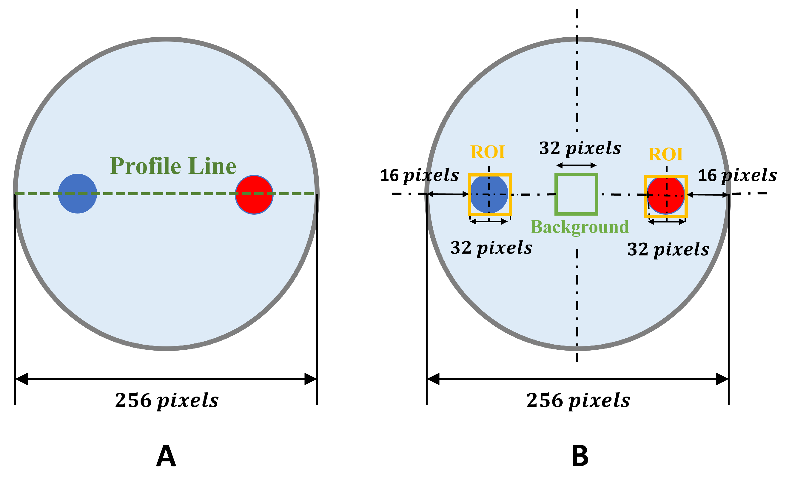
Refinement of the evaluation of various objects in EIT at multiple frequencies involves using profile lines that traverse the objects, as shown in Figure 2A. This method improves the understanding of how changes in frequency affect the contrast of materials in EIT images. The objectives of employing profile lines include:

• Evaluating frequency-dependent impedance: These profiles are instrumental in analyzing the impedance characteristics of materials at different frequencies. By intersecting various materials, they reveal impedance changes with frequency alterations.
• Quantifying contrast: The data from these profiles are crucial for quantitatively assessing the contrast of different materials. This analysis is key to understanding how EIT images distinguish between materials across the electromagnetic spectrum.
• Exploring a range of frequencies: The approach includes a wide spectrum of frequencies to comprehensively study how various materials appear in EIT images at different frequency levels, allowing for a detailed investigation of frequency-related effects.

This technique of using profile lines aims to deepen the understanding of EIT imaging, especially for materials with diverse electrical properties, potentially leading to significant advancements in various EIT applications and the study of frequency-dependent contrast in EIT.

In evaluating the quality of EIT images, sharpness and contrast parameters play crucial roles [35]. Sharpness, an essential metric for assessing clarity and resolution, is calculated using the gradient method. The formula is given by:

$$\mathrm{Sharpness}=\sqrt{\frac{1}{N}{\displaystyle \sum _{i=1}^N}{(\nabla I_i)}^2}$$

(2)

In this equation, $\nabla I_i$ represents the gradient of the image intensity at pixel i, and N is the total number of pixels. The sharpness value provides an average edge contrast across the image, reflecting EIT’s ability to accurately delineate boundaries and structures.

The contrast parameter is integral in evaluating the system’s ability to distinguish between regions of different electrical conductivities [36]. This capability is essential to differentiating between various materials or tissues. Contrast is often calculated based on the intensity values within the image using the following formula.

$$\mathrm{Contrast}=\frac{I_{\max }-I_{\min }}{I_{\max }+I_{\min }}$$

(3)

In Equation (3), $I_{\max }$ and $I_{\min }$ represent the maximum and minimum intensity values within the image, respectively. This calculation yields a normalized value, reflecting the degree of differentiation the EIT system can achieve between the highest and lowest conductivity regions.

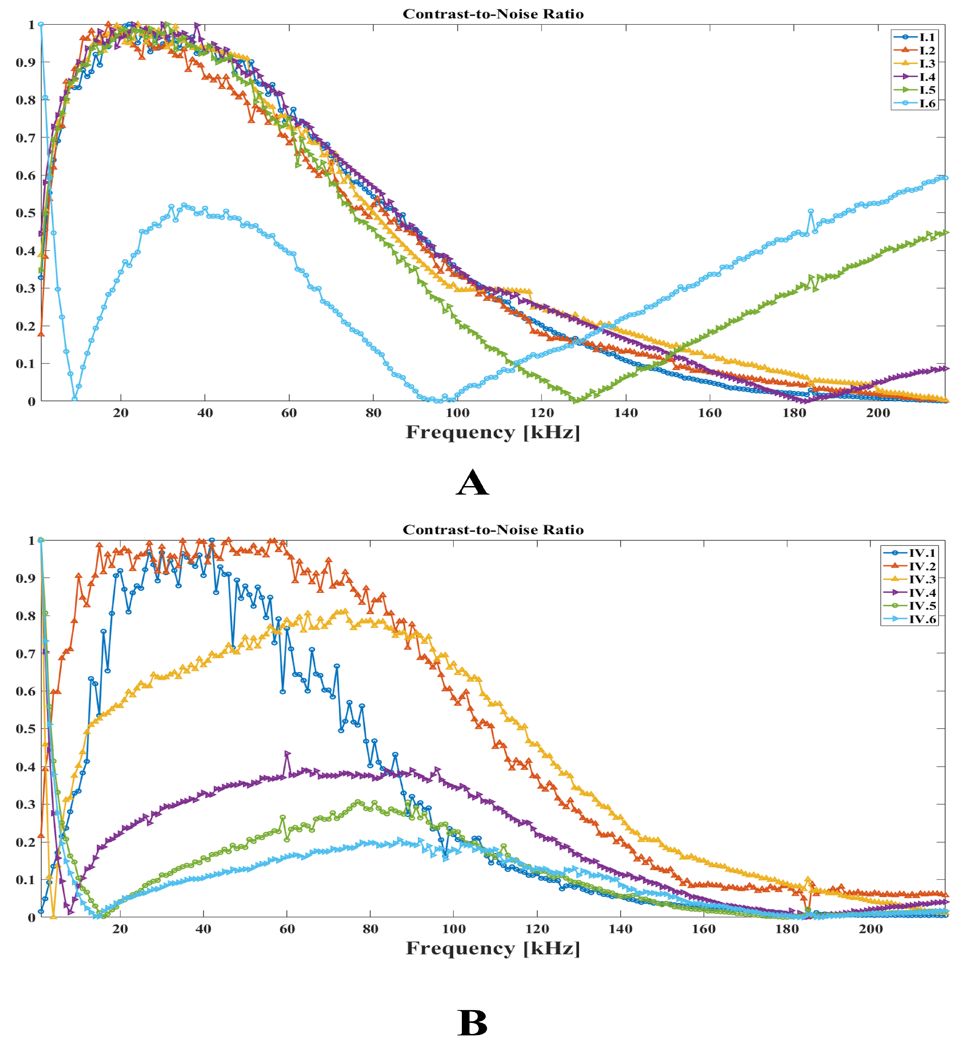
Regarding the analytical aspect of this investigation, the contrast-to-noise ratio (CNR) was used as a metric to evaluate the image quality and clarity across different frequency settings in EIT, as shown in Figure 2B [37,38]. CNR is a vital quantitative tool for measuring the object contrast within an image, distinguishing it from background noise. CNR can be calculated using the following formula:

$$\mathrm{CNR}=\frac{\left|{\mu }_{\mathrm{ROI}}-{\mu }_{\mathrm{bkg}}\right|}{{\sigma }_{\mathrm{noise}}}$$

(4)

In Equation (4), ${\mu }_{\mathrm{ROI}}$ is the mean impedance value within the Region of Interest (ROI) containing the object, ${\mu }_{\mathrm{bkg}}$ is the mean impedance value of the background, and ${\sigma }_{\mathrm{noise}}$ is the standard deviation of the noise in the background. This formula and its application are illustrated in the study, providing a comprehensive analysis of the EIT image quality at varying frequencies.

3. Results

In this study, the stability of the signal acquisition system was assessed. The test involved examining a precision resistor with a known value of 1 kΩ across the frequency range of 1 Hz to 500 kHz. The results indicate that the maximum deviation falls within the range of $993\Omega$ to 1.009 kΩ, with a corresponding standard deviation value of $3.0117$, as illustrated in Figure 3.

Figure 4 shows the SNR values derived from 208 measurements across 5 experiments. Each measurement involved 500 repetitions, and the SNR was calculated using Formula (1). All experiments consistently showed an SNR index exceeding 30 dB. Specifically, experiments conducted in a homogeneous environment (saltwater) (Figure 4A,B,D) exhibited a higher average SNR index compared to those in a non-uniform field (ground-meat environment) (III, V) (Figure 4C,E). This underscores the effectiveness of the signal acquisition system in facilitating additional experiments and assessments.

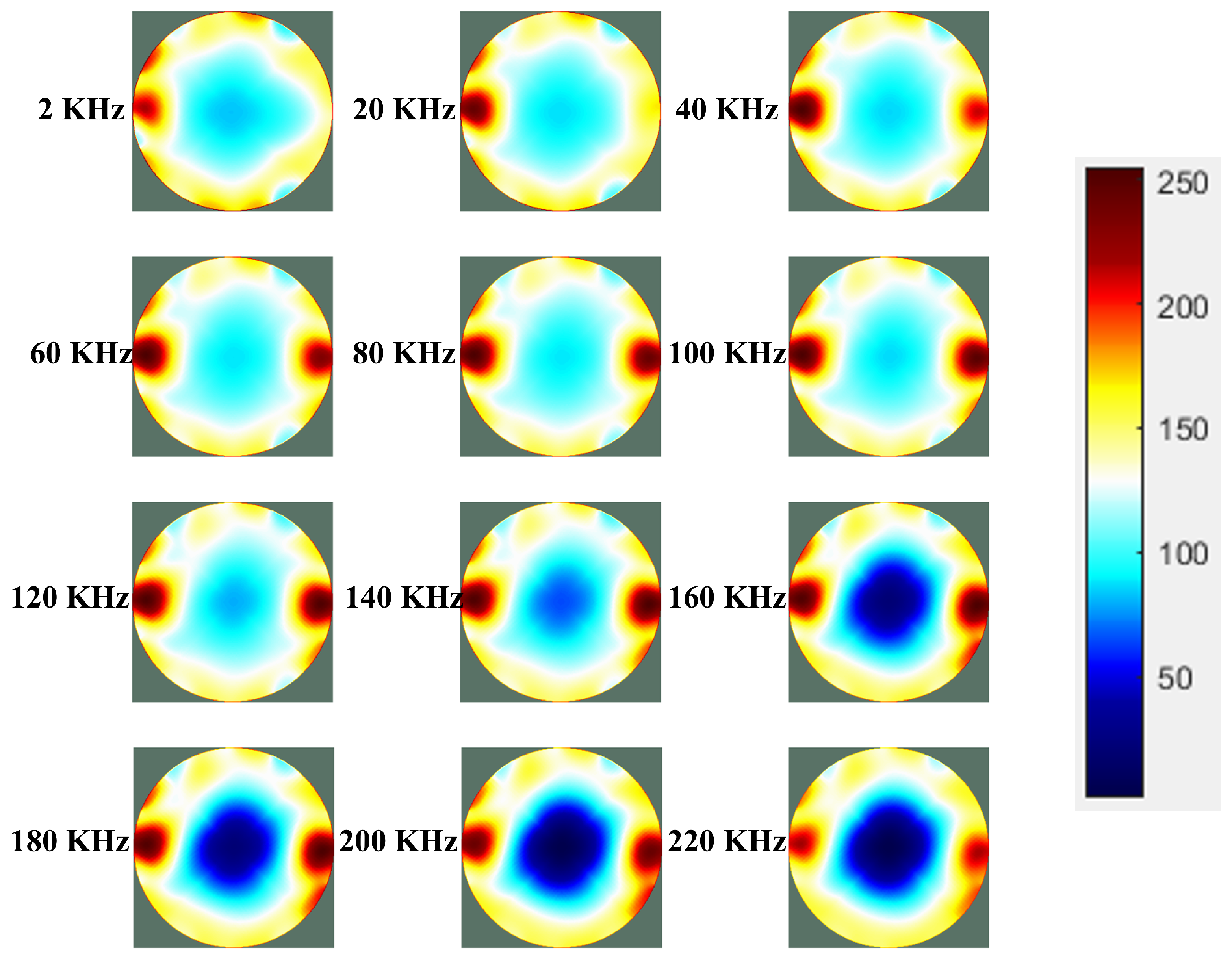
3.1. Experiment I

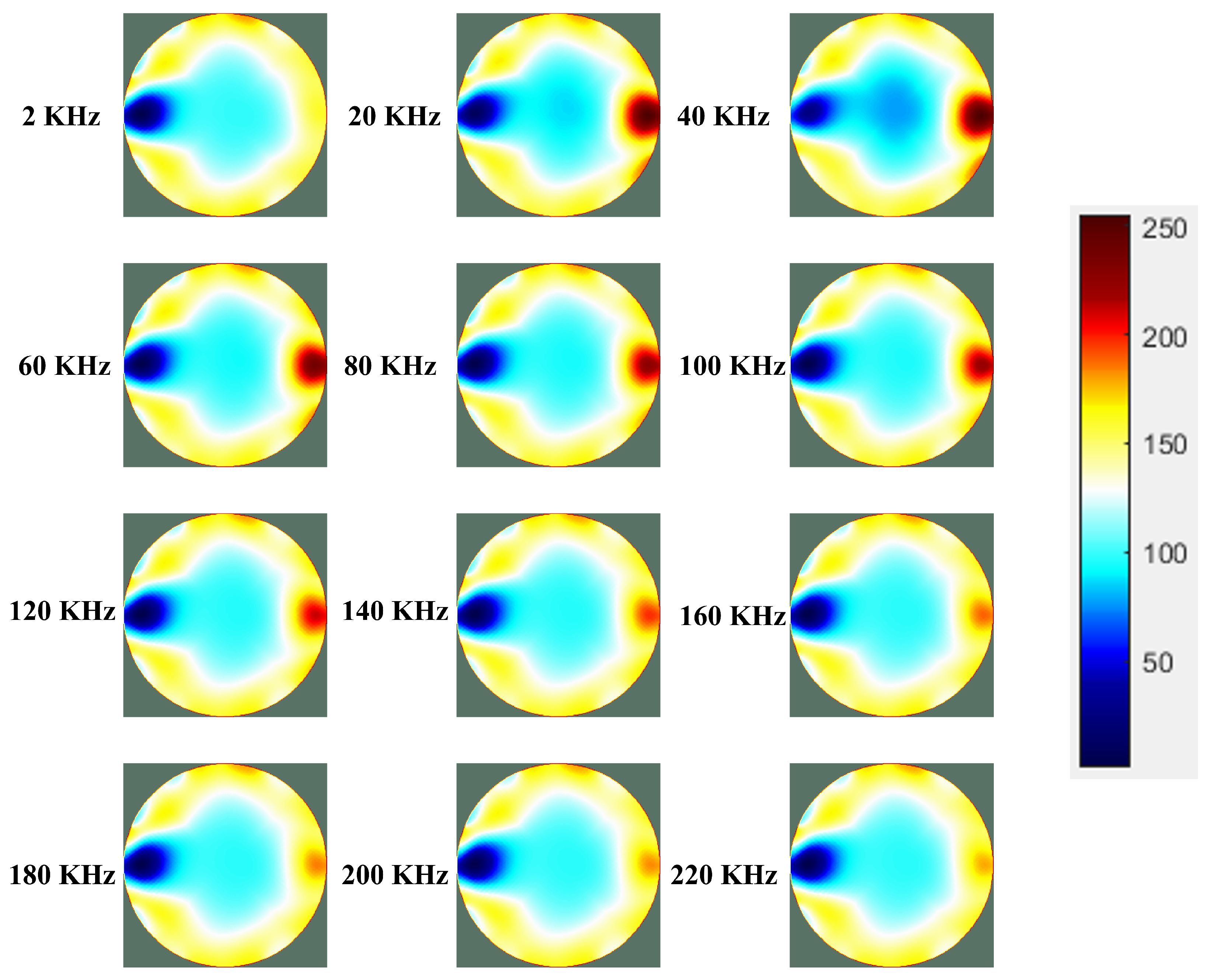
In the context of EIT, the experimental results depicted in Figure 5 and Figure 6 of Experiment I are employed to comprehend the dependent conductivity imaging, specifically for the copper material. Figure 5 illustrates the reconstructed conductivity cross-section of a phantom, acquired at frequencies spanning from 1 kHz to 220 kHz. The high-resolution $256\times 256$ pixel image distinctly depicts variations in conductivity across different frequencies, emphasizing the crucial impact of the frequency selection on improving the image clarity and detail in EIT.

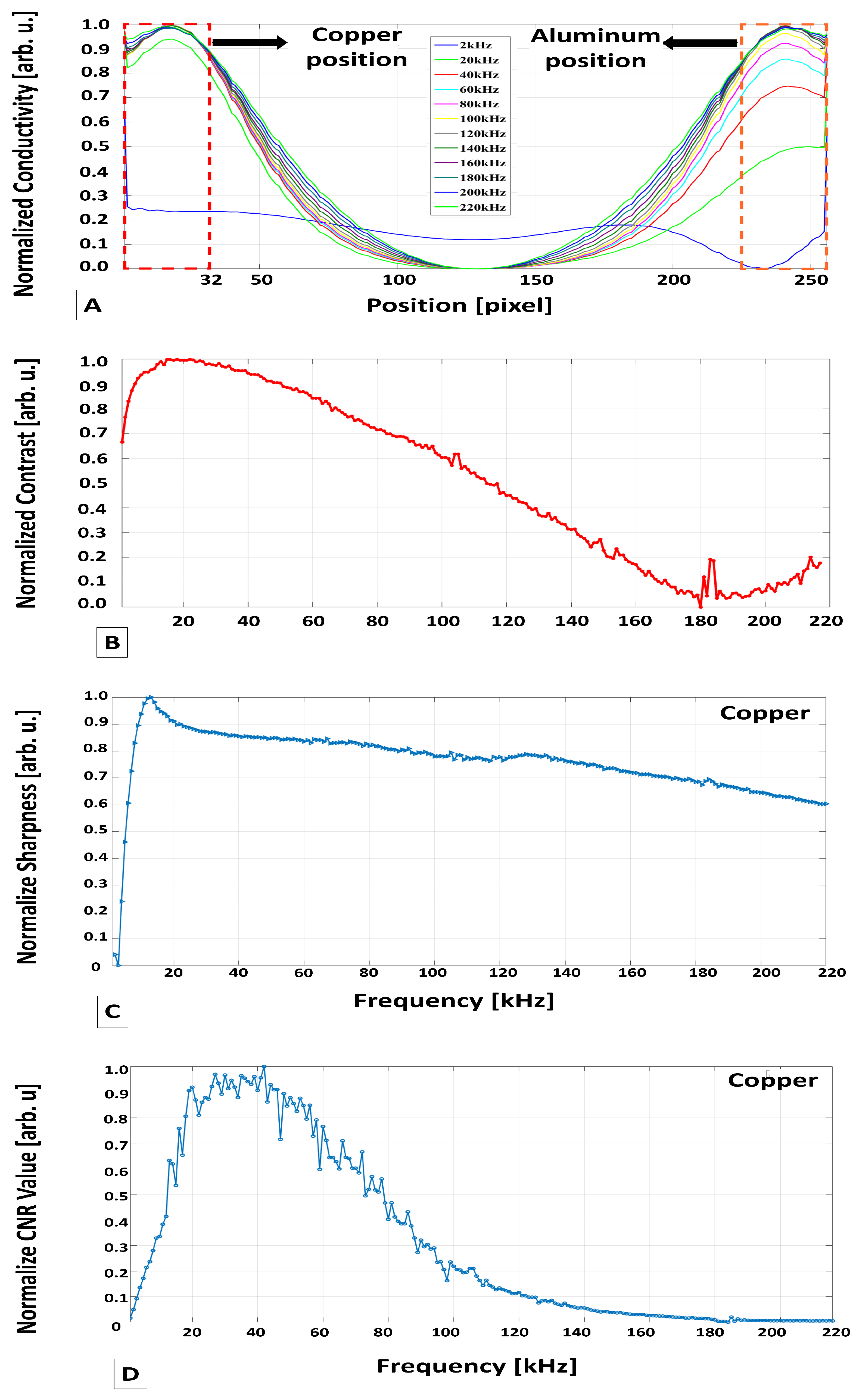
The further analysis in Figure 6A shows the profile line of normalized conductivity intensities along the 128th pixel row for Experiment I.1. The placement of the object spans pixels 1 to 32, with the profile line reaching its peak value at the 16th pixel. This aligns with the object’s center, showcasing the effective signal reception of the system. An essential observation involves the identification of the highest contrast values within the profile line, which occur in the frequency range that exceeds 2 kHz and extends to 40 kHz.

In Figure 6B, the normalized contrast values of the image are illustrated, highlighting the higher contrast in the frequency range of 10 kHz to 60 kHz with a threshold of $0.95$. This finding is supported by the analysis of two crucial normalized parameters: sharpness (Figure 6C) and CNR (Figure 6D). The peak values in both graphs consistently fall within the 15–38 kHz frequency window with a threshold of $0.95$, indicating that this range is most advantageous to achieve a higher contrast in EIT imaging for copper material.

3.2. Experiment II

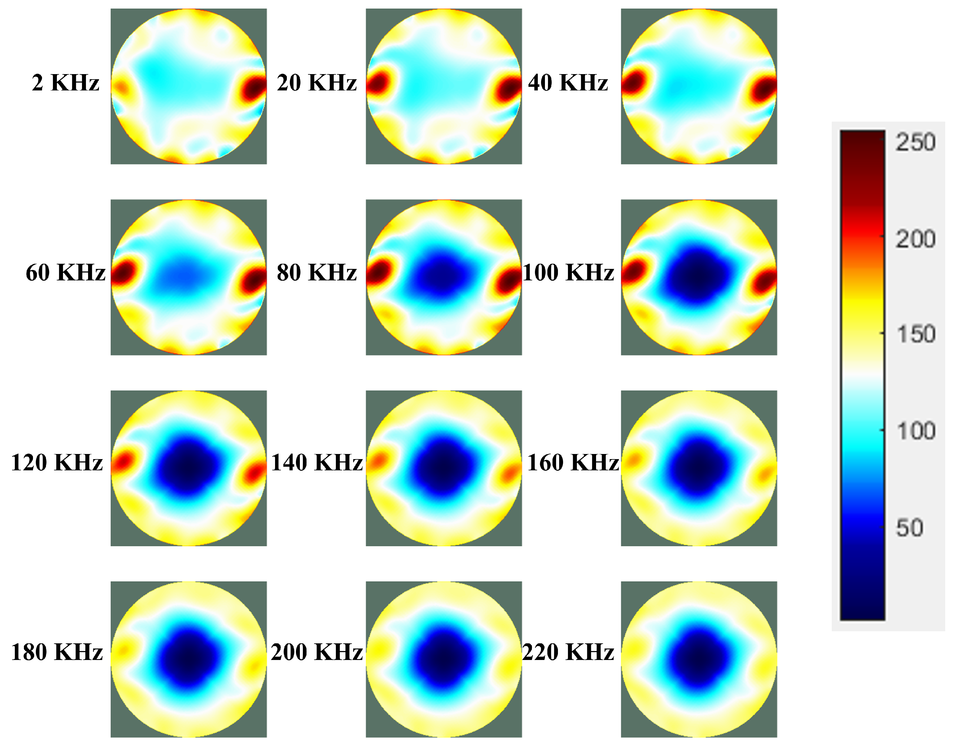
In Figure 7 and Figure 8, the results of Experiment II.1 are presented to evaluate how an electrically conductive material (aluminum) influences the frequency-dependent contrast behavior of copper within the same phantom. The reconstructed image in Figure 7 illustrates the normalized conductivity intensity distribution within the phantom, captured at a resolution of $256\times 256$ pixels.

In Figure 8A, the profile line of the normalized electrical conductivity intensities is highlighted along the 128th pixel row. Copper occupies pixels 1 to 32, while aluminum spans pixels 224 to 256. Peaks in the profile line occur at the 18th and 239th pixel numbers, indicating a deviation in the center of the objects by the second and first pixel, respectively. This observation confirms that both copper and aluminum exhibit significant contrast in their profile lines within the frequency range of 2–40 kHz.

In Figure 8B, the normalized contrast values of the images are illustrated. It is evident that the frequency range between 15 kHz and 35 kHz yields higher image contrast with a threshold of $0.95$. This conclusion is supported by the analysis of two key parameters: sharpness, illustrated in Figure 8C, and CNR, depicted in Figure 8D. Both parameters indicate that the frequency range spanning from 18 to 36 kHz is the most effective to achieve a high contrast in copper EIT imaging, maintaining a threshold of $0.95$. This particular range is especially significant for understanding the influence of the proximity of another conductive material, such as aluminum, on the contrast behavior of copper in EIT imaging.

3.3. Experiment III

In Figure 9 and Figure 10, the results of Experiment III.1 are presented, mirroring the methodology of Experiment II.1. In this iteration, the locations of the two objects were exchanged, and the phantom environment transitioned from a water-based medium to a ground-meat environment. The reconstructed image in Figure 9 shows the normalized electrical conductivity distribution of the cross-sectional phantom.

In Figure 10A, the profile line depicts the normalized electrical conductivity intensities along the 128th pixel row, spanning a frequency range of 1–220 kHz. The aluminum object occupies pixels 1 to 32, while the copper object occupies pixels 224 and 256. In particular, the peaks at the 18th (with a two-pixel deviation) and 240th positions in the profile lines correspond to the centers of the two objects. These findings highlight the effective signal-acquisition capability of the system in a non-homogeneous medium.

Figure 10B illustrates the normalized contrast values across the frequency spectrum from 1 to 220 kHz, using a threshold of $0.95$ to identify a practical frequency range from 14 to 37 kHz. This frequency range aligns with normalized sharpness parameters, ranging from 15 to 38 kHz, and normalized CNR parameters, ranging from 16 to 37 kHz, as shown in Figure 10C and Figure 10D, respectively. These results suggest that the identified frequency range to achieve a higher image contrast under the given experimental conditions provides valuable insights for EIT imaging in a heterogeneous environment.

3.4. Experiment IV

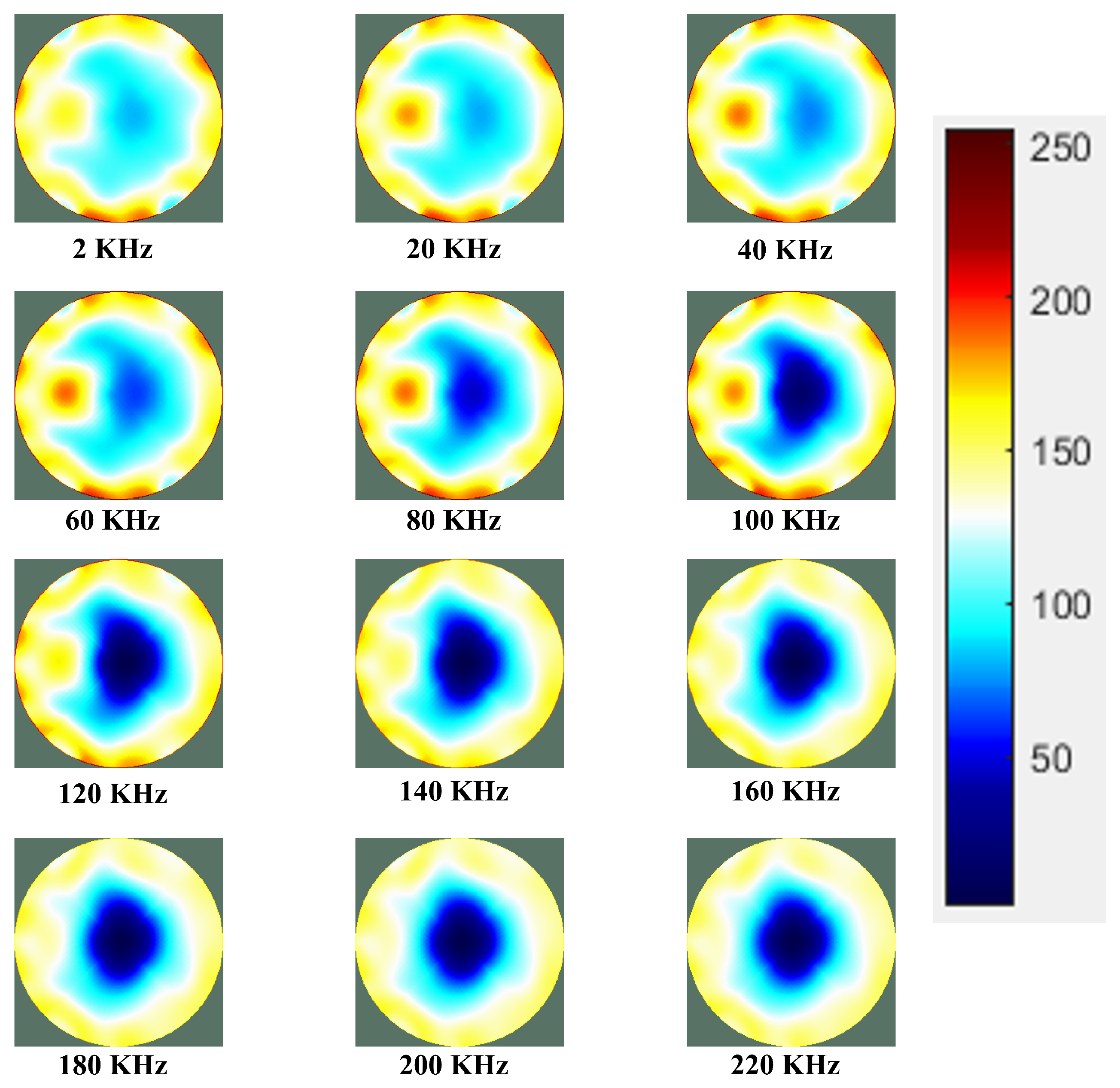
Figure 11 and Figure 12 depict the results of Experiment IV.I, which was carried out on acrylic resin samples immersed in a homogeneous environment (saltwater). Figure 11 presents a normalized cross-sectional reconstruction of the conductivity distribution in the phantom over the investigated frequency range (1–220 kHz). This illustration reveals minimal changes in object contrast as frequencies vary. The impedance contrast between plastic objects and their surroundings remains moderately low, resulting in limited alterations in contrast.

In Figure 12A, the normalized profile of the conductivity intensity is shown along the row of the 128th pixels. It is apparent that the profile lines exhibit a minimum point at the 20th pixel position (deviated by four pixels from the true center of the object) and are nearly identical. This consistency results from negligible conductivity changes within the surveyed frequency range. Figure 12B shows the normalized contrast with the threshold of $0.95$ and that the frequency range from 45 kHz to 80 kHz is with higher contrast.

Subsequently, Figure 12C,D illustrates the normalization of sharpness and CNR, respectively, along with their respective empirical frequency ranges of 50 kHz to 75 kHz and 47 kHz to 75 kHz. These analyses offer crucial insights into the frequency-dependent contrast characteristics of acrylic resin phantoms, contributing to a deeper understanding of the empirical frequency selection for enhanced resolution in the EIT imaging of acrylic resin.

3.5. Experiment V

Figure 13 and Figure 14 present the results of Experiment V.1, which was carried out on copper and acrylic resin within a heterogeneous medium (ground meat). In Figure 13, the normalized cross-sectional reconstruction image of the phantom conductivity is displayed. The image follows the patterns observed in Experiment I.1 for copper, showing high contrast in the frequency range of 20 to 40 kHz. Similarly, it aligns with the findings of Experiment IV.1 for acrylic resin, revealing minimal changes with varying frequencies.

In Figure 14A, the normalized conductivity profile along the 128th pixel row is presented. The profile shows a minimum value at the 19th pixel (three pixels away from the center of the acrylic resin object) and a maximum value at the 239th pixel (one-pixel deviation from the position of the copper object).

Similarly, the sharpness normalization index shown in Figure 14B indicates that the empirical frequency range for copper is 18–35 kHz, while for acrylic resin, it is 48–76 kHz. This is further supported by verification using the CNR normalization index in Figure 14C, where the empirical frequency range for copper is 20–37 kHz, and for acrylic resin, it is 46–75 kHz. Although some discrepancies exist, these results align with the conducted experiments, affirming the suitability of the selected frequency region with the contrast of conductive and non-conductive materials.

3.6. Assessing the Impact of Object Position in the Phantom on Empirical Frequency Selection

Figure 15 illustrates a cross-sectional reconstruction of the phantom in Experiment I within a homogeneous environment, examining the impact of the position of the object on the contrast within a specific frequency range. The results reveal a gradual decrease in object contrast as the distance from the electrode increases at the same survey frequency. In particular, the empirical frequency range, ranging from 15 to 40 kHz, aligns with the findings of previous experiments, emphasizing the robustness of this frequency window. Furthermore, Figure 16, Figure 17, Figure 18, Figure 19 and Figure 20 illustrate the impact of different object positions.

Figure 21A shows the variations in linear intensity through the CNR index, providing valuable information on contrast dynamics. This phenomenon suggests that the influence of object position on contrast is a significant factor within the explored frequency range. The consistent empirical frequency range from 15 to 40 kHz at different positions of objects indicates a robust characteristic, which underscores the reliability of this frequency window in achieving high contrast. Additionally, Figure 21B shows deviations in frequency ranges corresponding to the object’s shift toward the center in a heterogeneous environment. This shift leads to an expanded frequency range and a non-linear decrease in CNR value intensity. The dynamic adaptation of the empirical frequency range emphasizes the importance of considering environmental heterogeneity in optimizing contrast for EIT imaging in scenarios with varied material compositions. These findings improve our understanding of contrast dynamics in EIT and advance imaging methodologies, and provide insights for optimizing contrast in diverse scenarios.

This result illustrates the spatial impact of the object’s position on contrast and emphasizes the resilience of the empirical frequency range. The observed variations in linear intensity and the effects of heterogeneous environments introduce additional intricacies to the discourse, fostering a more detailed comprehension of contrast dynamics in EIT. These insights play an essential role in the advancement of imaging methodologies and present valuable factors to be considered in order to enhance contrast optimization in a multitude of scenarios.

4. Discussion

The analysis of the experiments in this study improves our understanding of the empirical frequency selection for different materials, specifically copper and resin in EIT. The discussions of each experiment collectively provide valuable insight into the frequency-dependent contrast behavior of these materials, guiding the identification of empirical frequency ranges.

For copper, Experiment I focused on revealing a distinct trend in frequency-dependent conductivity imaging. The reconstructed conductivity cross-section and profile line consistently demonstrated high contrast in the frequency range of 2–40 kHz. Normalized contrast, sharpness, and CNR supported this finding, indicating that the frequency window of 15–38 kHz is most advantageous for a higher contrast in EIT imaging for copper. The high contrast of copper in this range can be attributed to its favorable electrical conductivity properties, which enhance the impedance contrast with that of its surroundings. EIT captures variations in electrical conductivity particularly well within this frequency window, contributing to the observed high contrast.

In Experiment II, the influence of adjacent aluminum on the contrast behavior of copper was explored. Despite the presence of another conductive material, both copper and aluminum maintained a significant contrast in the frequency range identified from 18 to 36 kHz. This result helps understand the potential interference of nearby conductive materials and reaffirms the effectiveness of the chosen frequency range for the high-contrast EIT imaging of copper. This suggests that the mechanism driving the contrast is robust and resilient to the influence of neighboring conductive elements, which is crucial for anticipating and mitigating potential interference in real-world applications.

Experiments III and V, conducted in heterogeneous environments using a ground meat environment, provided valuable information on the frequency-dependent contrast behavior of copper and resin. With some deviation, the frequency range of 14–37 kHz provides an understanding of the better imaging parameters for EIT in complex environments with multiple conductive materials. Experiment V reinforced the trends observed in Experiment I.1 for copper and Experiment IV.1 for resin, highlighting the consistency of the empirical frequency range for contrast. This provides insight into the adaptability of the imaging system to complex conditions, underscoring the resilience of EIT and its potential for application in scenarios with varying material compositions.

For acrylic resin, Experiment IV, focusing on the resin in a homogeneous environment (salt water), revealed minimal changes in object contrast within the frequency range of 45–75 kHz. The normalized profile and analyses confirmed that this frequency window is used to achieve high contrast in the EIT imaging of the resin. This finding expands our understanding of frequency-dependent contrast characteristics in EIT imaging of non-conductive materials. Minimal changes in contrast within the identified empirical frequency range for resin suggest a consistent behavior of non-conductive materials. The mechanism underlying this behavior may involve the interaction of the electric field with the molecular structure of the resin, resulting in detectable but limited variations in impedance.

This study acknowledges specific limitations that merit discussion. First, the use of cylindrical samples may introduce considerations about the generalizability of the findings to more complex geometries. Cylindrical objects represent a simplified model, and the behavior of conductive and non-conductive materials in more intricate shapes may exhibit variations not captured in this study. Furthermore, the study focused on specific materials (copper and acrylic resin), and the results may not be universally applicable to a wider range of materials with diverse electrical properties. These limitations underscore the importance of further research that includes varied sample geometries and materials in order to improve the comprehensiveness and applicability of the findings. Additionally, the reconstruction method utilizing the EIDORS algorithm has proven effective, yet certain assumptions and parameters involved in the reconstruction process may introduce uncertainties. Further investigations into optimizing current patterns and refining reconstruction parameters are essential for advancing the precision and reliability of EIT imaging. The collective findings suggest that the empirical frequency range for copper lies between 15 and 38 kHz, while for acrylic resin, the range of 45–75 kHz is deemed empirical. These results provide parameters for selecting appropriate frequencies in EIT imaging scenarios involving different materials, enhancing the technique’s precision and applicability across diverse environments.

5. Conclusions

In summary, the in-depth exploration of frequency-dependent contrast in EIT has significantly advanced the understanding of imaging methodologies, particularly in scenarios involving materials with distinct electrical properties, as demonstrated by acrylic resin and copper. The conducted experiments offer insights into empirical frequency ranges for enhanced contrast, considering variables such as object position, adjacent materials, and heterogeneous environments. These findings contribute to essential considerations for optimizing EIT imaging strategies, deepening the understanding of contrast dynamics. As the intricacies of EIT applications are revealed, this research establishes a foundation for enhanced precision and applicability across diverse environments, unlocking the full potential of this imaging technique in real-world scenarios.

Optimized frequency selection in EIT holds promise for improving non-destructive inspection of copper welds in industries like energy and aerospace, potentially revolutionizing safety standards. Similarly, monitoring fluid flow in acrylic resin pipes could be transformed in sectors such as chemical processing, ensuring the safe and efficient handling of sensitive materials. The results reveal distinct empirical frequency bands for enhancing contrasts in specific materials: 15–38 kHz for conductive materials (copper) and 45–75 kHz for non-conductive materials (acrylic resin). Moreover, the potential for early skin cancer detection through EIT’s sensitivity to conductivity differences between healthy and cancerous tissues presents exciting possibilities in the medical field. Additionally, environmental applications, such as monitoring saltwater intrusion in coastal areas or detecting buried pipes and cables, could greatly benefit from EIT’s precision and non-invasive nature with optimized frequency selection.

Future EIT research should aim to enhance the applicability and understanding of this imaging technique. There is a compelling need to explore diverse sample geometries beyond the current focus on cylindrical samples so as to broaden generalizability. Additionally, investigating the frequency-dependent contrast behavior of a more extensive range of materials will provide insights, deepening the understanding beyond the current focus on acrylic resin and copper. Additionally, future endeavors should evaluate the adaptability of specific empirical frequency ranges in real-world applications, ensuring the practical relevance and robustness of the findings in various scenarios.