ADMM-1DNet: Online Monitoring Method for Outdoor Mechanical Equipment Part Signals Based on Deep Learning and Compressed Sensing

Abstract

To solve the problem that noise seriously affects the online monitoring of parts signals of outdoor machinery, this paper proposes a signal reconstruction method integrating deep neural network and compression sensing, called ADMM-1DNet, and gives a detailed online vibration signal monitoring scheme. The basic approach of the ADMM-1DNet network is to map the update steps of the classical Alternating Direction Method of Multipliers (ADMM) into the deep network architecture with a fixed number of layers, and each phase corresponds to an iteration in the traditional ADMM. At the same time, what differs from other unfolded networks is that ADMM-1DNet learns a redundant analysis operator, which can reduce the impact of outdoor high noise on reconstruction error by improving the signal sparse level. The implementation scheme includes the field operation of mechanical equipment and the operation of the data center. The empirical network trained by the local data center conducts an online reconstruction of the received outdoor vibration signal data. Experiments are conducted on two open-source bearing datasets, which verify that the proposed method outperforms the baseline method in terms of reconstruction accuracy and feature preservation, and the proposed implementation scheme can be adapted to the needs of different types of vibration signal reconstruction tasks.

1. Introduction

Online monitoring of mechanical equipment status is essential to extend equipment service life and ensure operational safety. However, general industrial equipment operated for a long time, and parts deteriorated slowly. With the increase in monitoring points and monitoring time, there are issues such as storage and transmission difficulties after the gradual accumulation of monitoring data [1,2]. Faced with this challenge, the industry urgently needs a reliable data compression method to effectively manage and store these large-scale monitoring data. In 2006, Donoho proposed compressed sensing (CS) [3], which provides a new idea for large-scale data storage and transmission. CS theory believes that if the signal itself is sparse or has a sparse property under a set of bases or dictionaries, then CS can recover the signal at a sampling rate significantly lower than the sampling rate specified by Nyquist theory [4,5,6,7].

In recent years, CS technology has developed rapidly and is widely used in quite a few fields, such as image processing [8,9], wireless communication [10], direction of arrival (DOA) estimation [11], and pipeline leakage detection [12]. Especially in industrial production, the CS reconstruction method based on acoustic emission signals [13,14,15] and multi-source composite fault signals [16,17] solved many practical industrial problems. These methods are generally applicable to the operation of mechanical equipment indoors or in stable environmental conditions, and signal acquisition is relatively easy to meet the sparse conditions of the compressed measurement. However, for mechanical equipment required to work in an open environment, the acquisition of monitoring signals is very vulnerable to environmental noise or human factors, such as fluctuation conditions [18,19], missing data from acquired signals [20,21,22], and high-noise interference [23], which results in the acquired signals not accurately reflecting the corresponding fault feature information.

In response to high-noise outdoor working conditions, some mechanical equipment monitoring and reconstruction methods have emerged. Generally, these methods are related to optimization-based methods [24,25], such as sparse optimization methods [26,27,28,29,30,31], waveform matching and dictionary learning-based methods [32,33,34,35], and multi-sensor fusion-based methods [36]. Although the need for accurate reconstruction of industrial vibration signals can be effectively addressed by the signal reconstruction methods described above, the disadvantages of the traditional method, such as having many parameters, slow convergence speed, and being prone to significant error at high compression ratios [37,38,39], are still difficult to avoid, resulting in the theory not being applied to the online monitoring demand of actual production equipment.

Recently, with the continuous development of deep learning, some scholars have proposed the application of neural networks to CS signal reconstruction, aiming to make full use of the advantages of neural networks to compensate for the shortcomings of traditional reconstruction algorithms. This work is usually divided into two main categories: data-driven methods and model-driven methods. The data-driven approach adapts to the data structure by adjusting the network models, such as DR2-Net networks [40], Deep Inverse networks [41], and CSNet networks [42]. The model-driven method is an idea that unfolds traditional CS methods into learning networks, first proposed in 2010 [43]. The article establishes the Learned Iterative Shrinkage Threshold Algorithm (LISTA) model on the basis of the ISTA [44] to solve sparse encoding problems. Since then, this idea has been widely applied to many signal and image problems [45,46,47]. In addition to the LISTA model, researchers also proposed unfolded network models such as ISTA-NET [48], LADM-NET [49], and AMP-Net [50]. These network models have obtained satisfactory results in the corresponding fields, but they do not involve the processing of high-noise and other interference components in the signal. This is because the network is sensitive to the sparse level of the signal and cannot be directly grafted into other outdoor, high-noise signal reconstruction fields.

Inspired by the CS signal reconstruction method based on an unfolded network [51,52,53,54], we propose a new signal reconstruction method, called ADMM-1DNet, for the online monitoring of bearing parts of mechanical equipment working in an open environment. Each iteration of the classical ADMM algorithm is unfolded into the layers of a deep neural network (DNN), and the network simultaneously learns a redundant analysis operator for sparse representation of the signal to address the impact of high-noise interference on reconstruction accuracy. The parameters of the ADMM algorithm are translated into network parameters. The network’s forward propagation is comparable to performing a limited number of iterations of the ADMM algorithm, followed by back-propagation training of the network to learn the model parameters from the training set. All parameters in the network are learned end-to-end, so the problem of large errors caused by relying on empirical values can be avoided. In addition, the establishment of the neural network follows the guidance of the traditional ADMM reconstruction algorithm. The expansion algorithm can not only efficiently reconstruct the signal but also make the signal reconstruction process have a certain interpretability [55,56].

The rest of this paper is organized as follows: two traditional convex optimal CS reconstruction algorithms are introduced in Section 2 and compared with the proposed method as the baseline method. Section 3 introduces the specific theory of the ADMM-1DNet network and the detailed signal online monitoring implementation scheme. In Section 4, the parameter setting and signal sparse level recovery performance of the network are explored on the simulation signal, and then the proposed method is compared with the traditional algorithm by taking the real bearing vibration signal as an example. Section 5 summarizes and discusses the results of this paper.

2. Theoretical Background

Generally, there are two kinds of algorithms to solve the reconstruction problem of the CS signal, i.e., the greedy algorithm [57,58] and the convex optimization algorithm [59,60,61]. Among them, the greedy algorithm is generally a heuristic method, which gradually builds the global optimal solution by selecting the local optimal solution every time. The convex optimization algorithm approximates the optimal solution step by step iteratively and has a convergence guarantee. For the problem with sparse structure, stable and accurate results can be obtained. The mathematical model for solving the signal inversion problem of compressed sensing under sparse conditions is defined as follows:

$$\underset{x\in {ℝ}^n}{\min }\frac{1}{2}{‖\mathit{A}x-y‖}_2^2+\lambda {‖\mathit{\phi }x‖}_1,$$

(1)

where $x\in {ℝ}^n$ is the signal to be reconstructed, A is the measurement matrix, y is the measurement value; λ is the regularization parameter, and φ is the transformation matrix.

2.1. CS Based on ISTA

The ISTA algorithm is a gradient-based approach in which the differentiable gradient is projected at each iteration and then reduced to a specific value by a threshold. Given the compression measurement y, ISTA achieves the reconstruction of the vibration signal by iterative solution (1) of gradient and signal. The signal to be reconstructed is updated by the x-shrinkage threshold operation, and the specific iterative formula is defined as follows:

$$Z^{\left(k\right)}=y-\mathit{A}{x}^{\left(k\right)},$$

(2)

$$x^{\left(k+1\right)}={\eta }_{\lambda }\left(x^{\left(k\right)}+\rho {\mathit{A}}^T{Z}^{\left(k\right)}\right).$$

(3)

where k is the number of iterations, $Z^{\left(k\right)}\in R^{M\times 1}$ is the immediate reconstruction signal of the $k\mathrm{th}$ iteration, ρ is the step size, η_λ (·) is the soft threshold function. The specific expression formula is defined as follows:

$${\left[{\eta }_{\lambda }\left(x\right)\right]}_i\triangleq \mathrm{sign}\left(x_i\right)\left(\left|x_i\right|-{\lambda }_i\right),$$

(4)

where λ_i is the threshold parameter, and sign(·) is the sign function.

The flow of the ISTA-based CS algorithm is shown in Figure 1. Where x₀ is the initialization value, r_k is the residual error obtained during the calculation process, and $\widehat{x}$ is the final reconstruction signal value.

Ref. [48] combines the above method with deep neural networks to propose the classic ISTA-NET method. In the following text, we will compare ISTA-NET with the proposed method in terms of overall performance.

2.2. CS Based on ADMM

The ADMM algorithm is also a classical convex optimization algorithm that introduces new variables to decompose the original objective function into several smaller subproblems for solution, and then the global optimal solution of the original objective function is obtained through the solution among the coordination sub-problems. ADMM has a broader definition for the solution of the inverse problem in Formula (1):

$$\underset{x\in {ℝ}^n}{\min }\frac{1}{2}{‖\mathit{A}x-y‖}_2^2+{\displaystyle \sum _{i=1}^C{\lambda }_i}g\left({\mathit{D}}_{i}x\right),$$

(5)

where g(·) is the nonlinear regularization parameter, and D_i is the transformation matrix. ADMM introduces the dyadic variable Z, which transforms Equation (5) into the following:

$$\begin{array}{l}\underset{x,{\left\{z\right\}}_{i=1}^C}{\min }\frac{1}{2}{‖Ax-y‖}_2^2+{\displaystyle \sum _{i=1}^C{\lambda }_i}g\left(z_i\right),\\ \mathrm{s}.\mathrm{t}.z_i={\mathit{D}}_{i}x\left(\forall i\right).\end{array}$$

(6)

Its corresponding Tseng generalized Lagrangin function is defined as follows:

$$L_{\rho }\left(x,z,{\epsilon }_i\right)=\frac{1}{2}{‖\mathit{A}x-y‖}_2^2+{\displaystyle \sum _{i=1}^C{\lambda }_i}g\left(z_i\right)+\frac{{\rho }_i}{2}{‖{\mathit{D}}_i-z_i+{\epsilon }_i‖}_2^2,$$

(7)

where ε_i is a binary variable, and ρ is a penalty parameter. ADMM method is obtained by alternately minimizing Equation (7) with bivariate updating, as follows:

$$\left\{\begin{array}{l}{X}^k:x^{\left(k\right)}={\left({\mathit{A}}^T\mathit{A}+{\displaystyle \sum _{i=1}^C{\rho }_i}{\mathit{D}}_i^T{\mathit{D}}_i\right)}^{-1}\left[{\mathit{A}}^{T}y+\left.{\displaystyle \sum _{i=1}^C{\rho }_i{\mathit{D}}_i^T\left(z_i^{(k-1)}-{\epsilon }_i^{(k-1)}\right)}\right]\right.\\ Z^k:z_i^k=S\left({\mathit{D}}_i{x}^{\left(k\right)}+{\epsilon }_i^{(k-1)};{\lambda }_i/{\rho }_i\right)\\ M^k:{\epsilon }_i^k={\epsilon }_i^{(k-1)}+\eta \left({\mathit{D}}_i{x}^{\left(k\right)}-z_i^{(k)}\right)\end{array}\right.,$$

(8)

where n_i is a constant parameter, and S(·) is a proximal mapping with parameter λ.

2.3. CS Based on ADMM + K-SVD

The mathematical model of the K-SVD dictionary learning algorithm is as follows:

$${‖Q-\mathit{D}\mathit{X}‖}_F^2=‖Q-{\displaystyle \sum _{j=1}^k{d}_j{\mathit{X}}_T^j}‖={‖\left(Q-{\displaystyle \sum _{j\ne k}{d}_j{\mathit{X}}_T^j}\right)-d_k{\mathit{X}}_T^{(k)}‖}_F^2={‖E_{\left(k\right)}-d_{\left(k\right)}{\mathit{X}}_T^{\left(k\right)}‖}_F^2,$$

(9)

where Q is the sample signal, D is the original dictionary, X is the sparse vector matrix and E_(k) is the residual. The de-zero contraction of ${\mathit{X}}_T^{(k)}$ yields $E_{(k)}^R$, then performs singular value decomposition, yielding the following:

$$E_{(k)}^R=\mathit{U}\Delta V^T.$$

(10)

The dictionary training process uses the elements in the U-matrix obtained by decomposition to assign values to the atomic training in dictionary D one by one.

It has been proven in the literature that the CS method based on K-SVD has the best reconstruction performance using an empirical dictionary as the initial dictionary [62,63]. The steps of the CS reconstruction signal method based on ADMM + K-SVD algorithms are shown in

Table 1. CS based on ADMM + K-SVD.

CS Based on ADMM + K-SVD
Step 1: The monitoring end receives the observation y, and the reference vibration signal is used as a training sample to obtain the initial dictionary D0.
Step 2: The ADMM algorithm is used to solve the optimization problem in Equation (1), resulting in the initial sparse approximation coefficients θ0. Solving for ỹ0 = D0θ0. gives the initial reconstructed signal data.
Step 3: Update the sparse transformation dictionary D with the K-SVD dictionary learning algorithm, and use the updated dictionary D to make a sparse representation of the preliminary reconstructed data from the previous step.
Step 4: Solve the updated sparse coefficients θi with the ADMM algorithm to update ỹi = Diθi.
Step 5: Take the data obtained in step 2 as the input data for the next iteration; repeat Steps 3 and 4 until the algorithm converges. Output the reconstructed data ỹ to realize the vibration signal reconstruction.

.

3. The Method Proposed in This Paper

3.1. ADMM-1DNet

For the outdoor high-noise signal reconstruction problem, the compressed measured value y according to CS theory is shown in Equation (11). Where the original signal $x\in {ℝ}^n$, $e\in {ℝ}^m,m<n$ corresponds to the noise in the acquired signal and ${‖e‖}_2\le \eta$.

$$y=\mathit{A}x+e.$$

(11)

We assume that there exists a redundant sparse transformation $\mathit{\Phi }\in {ℝ}^{N\times n}(N>n)$ called the analysis operator that makes Φx approximately sparse. To obtain x, a common approach is to transform it into solving the l₁-minimization problem as follows:

$$\underset{x\in {ℝ}^n}{\min }{‖\mathit{\Phi }x‖}_1\mathrm{s}.\mathrm{t}.{‖\mathit{A}x-y‖}_2\le \eta .$$

(12)

The ADMM algorithm is a classical convex optimization algorithm for solving the problem of Equation (12), which considers the equivalent generalized LASSO form of Equation (12), as follows:

$$\underset{x\in {ℝ}^n}{\min }\frac{1}{2}{‖\mathit{A}x-y‖}_2^2+\lambda {‖\mathit{\Phi }x‖}_1.$$

(13)

Introducing the dual variables $z,u\in {ℝ}^N$, Equation (13) is transformed into the following:

$$\underset{x\in {ℝ}^n}{\min }\frac{1}{2}{‖\mathit{A}x-y‖}_2^2+\lambda {‖z‖}_1,\mathrm{s}.\mathrm{t}.\mathit{\Phi }x-z=0.$$

(14)

The optimization problem of Equation (14) can be solved using an iterative scheme of ADMM for the penalty parameters ρ > 0, $k\in \mathbb{N}$ and the initial points (x⁰, z⁰, u⁰):

$$x^{(k+1)}={\left({\mathit{A}}^T\mathit{A}+\rho {\mathit{\Phi }}^T\mathit{\Phi }\right)}^{-1}\left({\mathit{A}}^{T}y+\rho {\mathit{\Phi }}^T\left(z^{\left(k\right)}-u^{\left(k\right)}\right)\right),$$

(15)

$$z^{(k+1)}=S_{\lambda /\rho }\left(\mathit{\Phi }{x}^{(k+1)}-u^{\left(k\right)}\right),$$

(16)

$$u^{\left(k+1\right)}=u^{\left(k\right)}+\mathit{\Phi }{x}^{\left(k+1\right)}-z^{\left(k+1\right)}.$$

(17)

Iterative steps (15)–(17) converge to the solution of Equation (14) [54], i.e., ${‖\mathit{A}{x}^{\left(k\right)}-y‖}_2^2+{‖z^{\left(k\right)}‖}_1\to p^{\ast }$ and $\mathit{\Phi }{x}^{\left(k\right)}-z^{\left(k\right)}\to 0$ as $k\to \infty$.

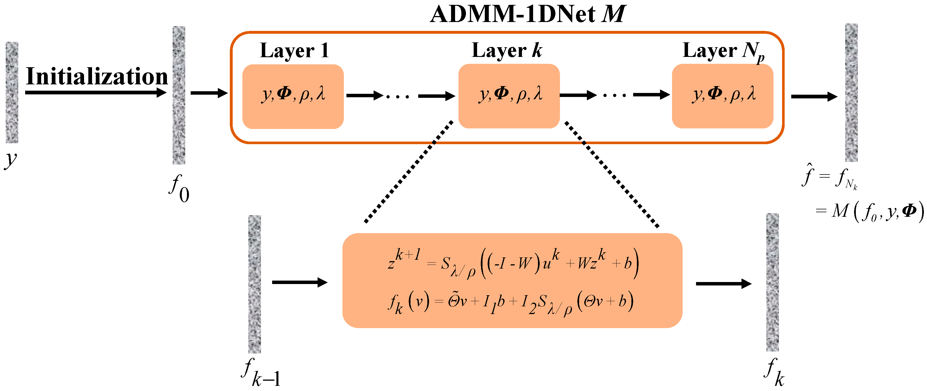
The idea of ADMM-1DNet is to map the aforementioned ADMM iterative scheme into a multilayer DNN, where each layer corresponds to an iteration of ADMM. The first Equation (15) is transformed into the update rules (16) and (17), and the second Equation (16) into (17).

$$\begin{array}{l}{u}^{(k+1)}=\left(I-W\right)u^{\left(k\right)}+W{z}^{\left(k\right)}+b-S_{\lambda /\rho }\left(\left(-I-W\right)u^{\left(k\right)}+W{z}^{\left(k\right)}+b\right),\\ z^{(k+1)}=S_{\lambda /\rho }\left(\left(-I-W\right)u^{\left(k\right)}+W{z}^{\left(k\right)}+b\right)\end{array}$$

(18)

where

$$W=\rho \mathit{\Phi }{\left({\mathit{A}}^T\mathit{A}+\rho {\mathit{\Phi }}^T\mathit{\Phi }\right)}^{-1}{\mathit{\Phi }}^T\in {ℝ}^{N\times N},$$

(19)

$$b=b(y)=\mathit{\Phi }{({\mathit{A}}^T\mathit{A}+\rho {\mathit{\Phi }}^T\mathit{\Phi })}^{-1}{\mathit{A}}^{T}y\in {ℝ}^{N\times 1}.$$

(20)

We introduce $v^{\left(k\right)}=\left[u^{\left(k\right)};z^{\left(k\right)}\right]\in {ℝ}^{2N\times 1}$ and set $\Theta =(-I-W|W)\in {ℝ}^{2N\times 1}$ and $\Lambda =(I-W|W)\in {ℝ}^{N\times 2N}$ to get the following:

$$v_{(k+1)}=\left(\begin{array}{c}\Lambda \\ O_{N\times 2N}\end{array}\right)v_{(k)}+\left(\begin{array}{c}b\\ 0\end{array}\right)+\left(\begin{array}{c}-S_{\lambda /\rho }(\Theta v_{(k)}+b)\\ S_{\lambda /\rho }(\Theta v_{(k)}+b)\end{array}\right).$$

(21)

Setting $\tilde{\Theta }=\left[\Lambda ;O_{N\times 2N}\right]\in {ℝ}^{2N\times 2N}$, $I_1=\left[I_{N\times N};O_{N\times N}\right]\in {ℝ}^{2N\times 2N}$ and $I_2=\left[-I_{N\times N};I_{N\times N}\right]\in {ℝ}^{2N\times N}$, transform Equation (21) into the following:

$$v_{(k+1)}=\tilde{\Theta }{v}_{(k)}+I_{1}b+I_2{S}_{\lambda /\rho }(\Theta v_{(k)}+b).$$

(22)

Based on the above equation, the ADMM algorithm is expanded to an L-layer neural network is defined as follows:

$$f_1(y)=I_{1}b(y)+I_2{S}_{\lambda /\rho }(b(y)),$$

(23)

$$f_k(v)=\tilde{\Theta }v+I_{1}b+I_2{S}_{\lambda /\rho }(\Theta v+b),k=2,\dots ,L$$

(24)

where $\mathit{\Phi }$ is trained as a trainable parameter, denote L such layers (all having the same $\mathit{\Phi }$) as

$$f_{\Phi }^L(y)=f_L\circ \cdots \circ f_1(y).$$

(25)

Applying the radiation mapping T driven by Equation (15) to the final layer of the neural network yields the final output $\widehat{x}$, i.e.,

$$\widehat{x}=T\left(f_{\Phi }^L\left(y\right)\right)={\left({\mathit{A}}^T\mathit{A}+\rho {\mathit{\Phi }}^T\mathit{\Phi }\right)}^{-1}\left({\mathit{A}}^{T}y+\rho {\mathit{\Phi }}^T\left(z^L-u^L\right)\right),$$

(26)

where $\left[u^L;z^L\right]=v_L$, in order to clip the output when the number of paradigms is out of range, it is necessary to add an additional function $\sigma :{ℝ}^n\to {ℝ}^n$ defined as: if ${‖x‖}_2\le B_{\mathrm{out}}$, then σ(x) = x, otherwise $\sigma (x)=B_{\mathrm{out}}x/{‖x‖}_2$, where $B_{\mathrm{out}}>0$ is a fixed constant. A hypothetical class is introduced containing the functions used that can be realized by ADMM-1DNet:

$$H^L=\left\{\sigma \circ h:{ℝ}^m\mapsto {ℝ}^n:h(y)=T(f_{\Phi }^L(y)),\right.\left.\mathit{\Phi }\in {ℝ}^{N\times n},N>n\right\}.$$

(27)

Given the above-hypothesized class and a set $S={\left\{\left(y_i,x_i\right)\right\}}_{i=1}^s$ containing S training samples, ADMM-1DNet yields a function $h_s\in H^L$ that aims at reconstructing x from y = Ax. Figure 2 gives a schematic diagram of ADMM-1DNet, where the operations of each block follow Equations (23) and (24).

Input Φ, ρ, and λ into the ADMM-1DNet network as parameters. So that they can learn adaptively rather than remaining constant during the training process. So here Φ^T is actually not a transpose of Φ in the strict sense.

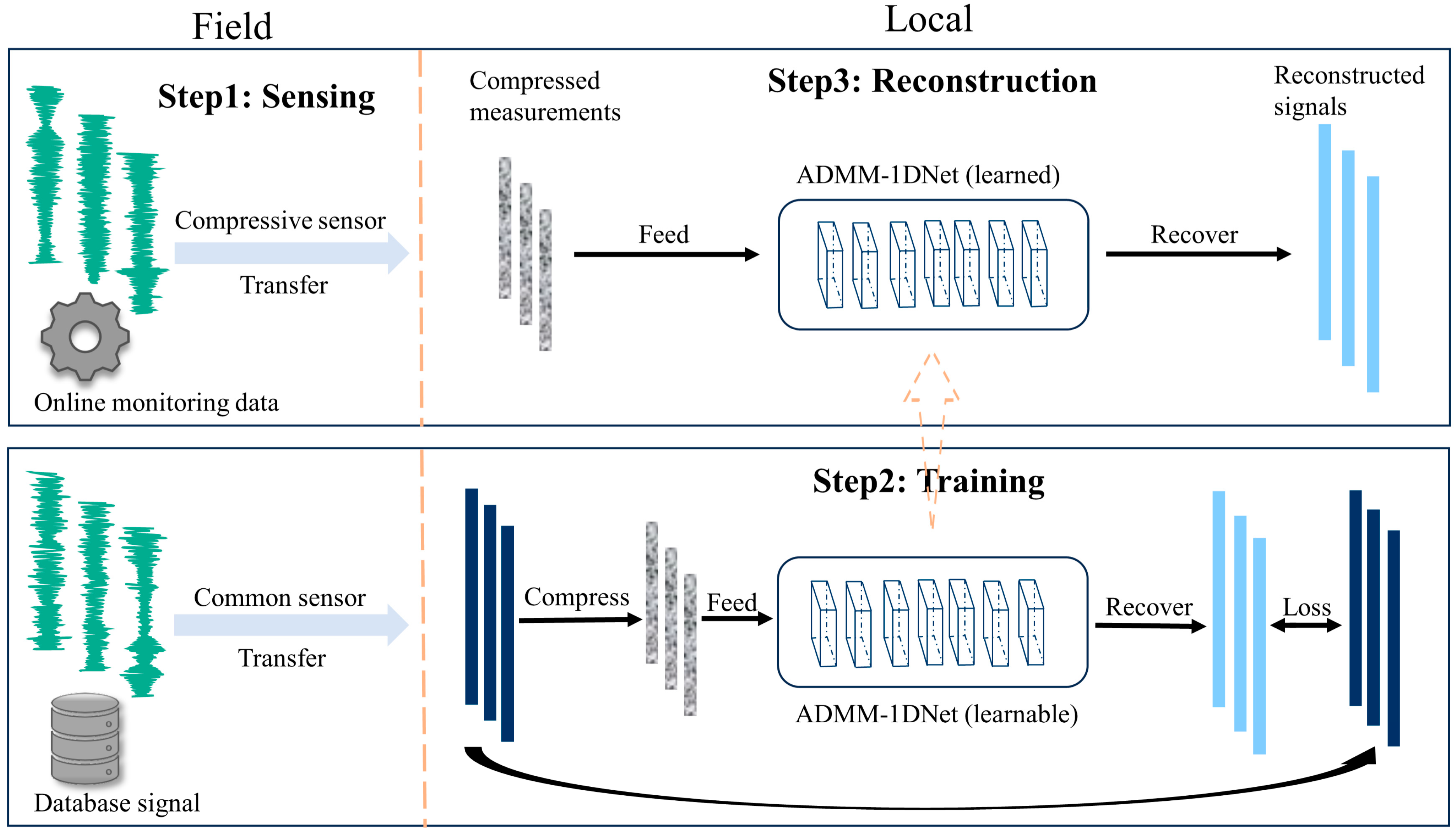
3.2. Signal Online Monitoring Scheme Design

The implementation scheme of ADMM-1DNet mechanical equipment component vibration signal reconstruction based on CS can be realized in the following three steps:

Step 1 The sensors collect and compress bearing vibration signals y and then transmit the signals to the local data center.

Step 2 The local data center uses the collected historical data to train the ADMM-1DNet network model, with the training guidelines following the settings in Section 4.2.1.

Step 3 The trained network accepts the data from Step 1, reconstructs the compressed measurement values, and outputs the reconstructed signal $\widehat{x}$.

As shown in Figure 3, the detailed online monitoring scheme for mechanical equipment component signals based on ADMM-1DNet is provided.

4. Experiment

4.1. Evaluation Indicators

In order to quantify the difference between x_i and ${\widehat{x}}_i=h_s(y_i),i=1,\dots ,s,$ we choose to use the training and the testing mean squared error as metrics to assess the reconstruction performance, defined as follows:

$$T_{\mathrm{train}}=\frac{1}{s}{\displaystyle \sum _{i=1}^s{‖h\left(y_i\right)-x_i‖}_2^2}$$

(28)

$$T_{\mathrm{test}}=\frac{1}{d}{\displaystyle \sum _{i=1}^d{‖h\left({\tilde{y}}_i\right)-{\tilde{x}}_i‖}_2^2}$$

(29)

$D={\left\{\left({\tilde{y}}_i,{\tilde{x}}_i\right)\right\}}_{i=1}^d$ is a set of data used for testing, containing d samples that were not used during the training phase. The data center reconstructs the outdoor collection data using the network model trained on historical data, and the closer the outdoor data reconstruction effect is to the training reconstruction effect the stronger the network generalization ability. Therefore, the generalization ability of the network by comparing the difference T_gen between the average training mean square error and the average testing mean square error, the T_gen is defined as follows:

$$T_{\mathrm{gen}}=\left|T_{\mathrm{test}}-T_{\mathrm{train}}\right|$$

(30)

Peak signal-to-noise ratio PSNR (in dB), compression ratio r and algorithm iteration Time (t) are used as evaluation metrics to measure the other performance of the network, PSNR is defined as follows:

$$\mathrm{PSNR}=10\lg \left[f_{\max }^2/\left(\frac{1}{N}{\displaystyle \sum _{i=1}^N{\left(f_i-{\widehat{f}}_i\right)}^2}\right)\right]$$

(31)

where f denotes the original signal, $\widehat{f}$ denotes the reconstructed signal, and f_max denotes the largest component of the vector f. The higher the value of the reconstruction signal-to-noise ratio, the better the reconstruction effect. The compression ratio r is defined as follows:

$$r=m/n$$

(32)

where n is the original signal length and m is the compressed signal length. The smaller the compression rate r, the higher the degree of signal compression.

The time taken by the algorithm to reconstruct the signal called the algorithm convergence Time (t), is used to characterize the complexity of the algorithm and as a reference for comparing the performance of different algorithms.

4.2. Simulated Signal Experiment

4.2.1. Network Parameters Setting Method

To explore the method of setting ADMM-1DNet network adaptation parameters and develop a more reasonable online monitoring implementation scheme, simulation signals were used for experimental research. The signal formula is defined as follows:

$$S(t)=0.1\sin (100\pi t+0.2\cos (40\pi t))+0.2\cos (250\pi t)+\eta (t)$$

(33)

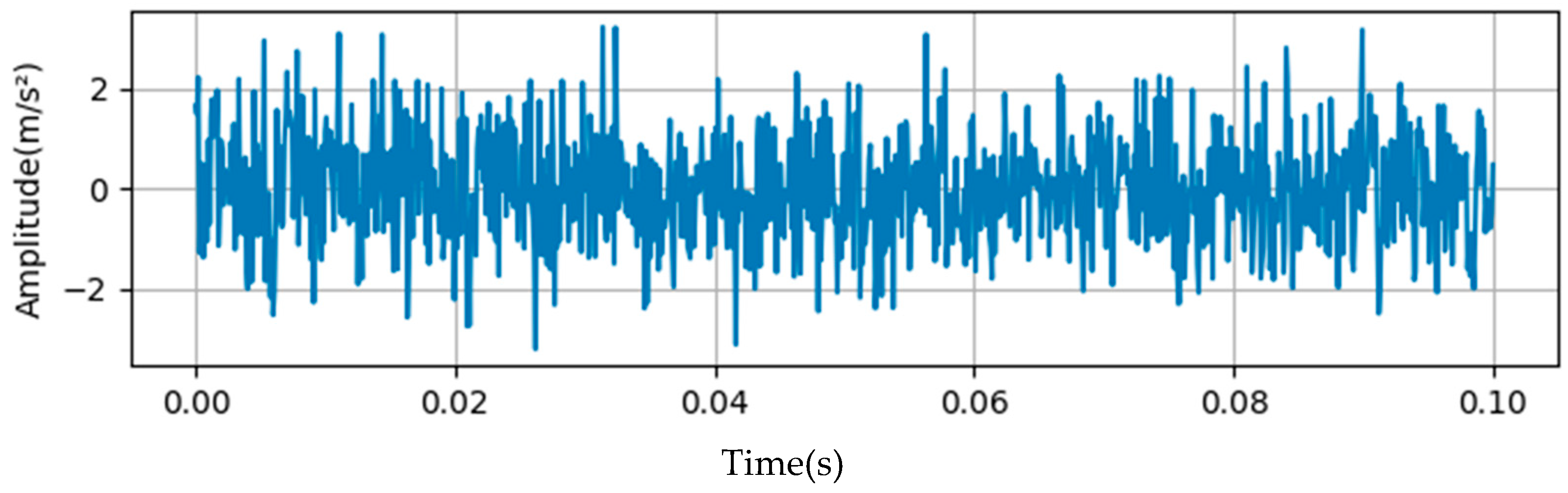
The signal is formed by the superposition of the frequency modulation component and cosine component, where the fundamental frequency is 50 Hz, the modulation frequency is 20 Hz, the frequency of the cosine component is 125 Hz, η(t) is a white noise term complying with normal distribution, the intensity is 1, and the time domain waveform of some signals is shown in Figure 4. In practical application, we can directly obtain the measured value instead of the original data. Therefore, ADMM-1DNet cannot acquire the prior knowledge from the test data, and another training set is required to provide the prior knowledge. To simulate this, 1024 sampling points in the experiment were defined as one signal unit and a training set containing 1200 signal units and a test set of 240 signal units were generated as experiment samples. The experiment r is now set to 20%.

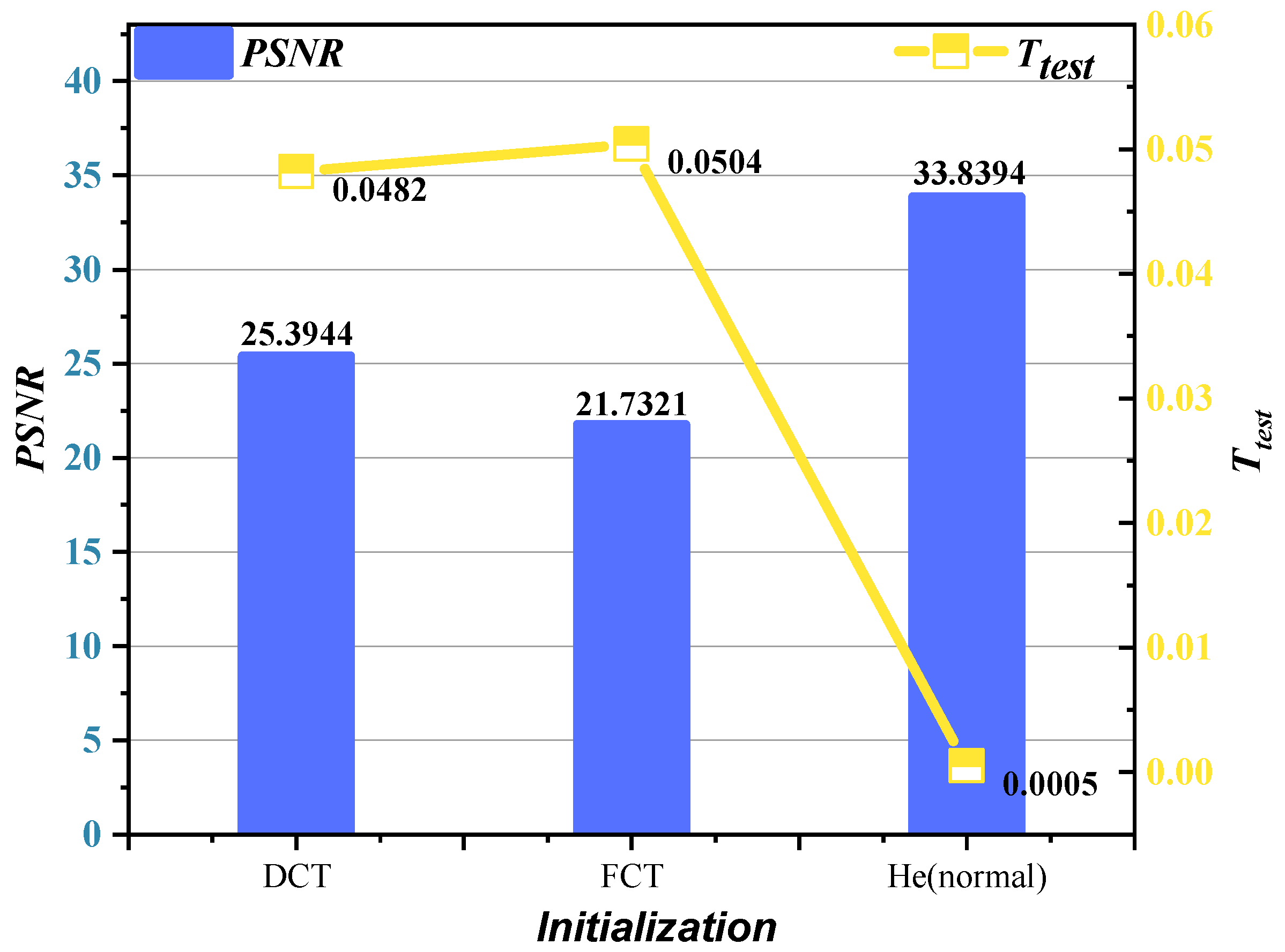
Firstly, we explore the initialization method of network redundancy analysis operator Φ and select three initialization methods, namely, discrete cosine transform (DCT dictionary), Fourier transform (FCT dictionary), and the He (normal) method for the experiment. Figure 5 shows the restructuring effect of the three initialization methods. It can be seen that the restructuring T_test obtained by using the He (normal) initialization method is the minimum, and the restructuring PSNR performance of the He (normal) method is significantly better than the other two methods. This indicates that when the He (normal) method is chosen to initialize Φ, the noise level of the reconstructed signal is relatively reduced and closer to the original signal.

The reconstruction accuracy is the primary index to judge the performance of the reconstruction algorithm, and then the reconstruction speed shall be considered. The experiment explores the relationship between the number of network expansion layers, signal reconstruction T_test, and network convergence time, and the results are shown in Figure 6. Using three different color balls to represent the results of network iterations 80, 90, and 100, respectively, it can be observed that when the number of unfolding layers is 4 or more, the reconstruction T_test is the lowest and gradually converges, indicating that the setting of four layers is more effective in achieving higher reconstruction accuracy. The same results are obtained with both 90 and 100 iterations when the number of layers is 4, but 90 iterations take less time. Experimentally setting the empirical network training parameters to 4 layers and 90 iterations is a better compromise scheme, as required by the actual situation.

Through simulation experiments, the best reconstruction performance of the network can only be achieved when different types of signals are configured with appropriate parameters. When training the network in the local data center, the network parameters should be adjusted one by one according to the principle of control variables. The parameter configuration process can be done automatically by the embedded program, and then the error and time cost caused by manual adjustment can be avoided. This “tailored” approach to network parameter training is not only more reliable than traditional static or empirically based parameter configuration methods but also allows the network to be adapted for a wide range of specific vibration signal reconstruction tasks.

In this study, the He (normal) method was used to initialize the redundant analysis operator Φ. The network deployment layers are all four layers, corresponding to four stages in the reconstruction process. Set (ρ, λ) = (1, 10⁻⁴) and Φ, ρ and λ are the same among all layers.

4.2.2. Sparsity Recovery Performance Analysis

For bearing parts of mechanical equipment operating outdoors, some fault features are buried in the noise, which disturbs the signal reconstruction process of CS. The more non-zero values in the reconstructed signal overlap with the original signal, the more noise tolerance the algorithm has. The ratio of non-zero elements in the signal can be expressed by the signal sparsity level L_S in Equation (34).

$$\begin{array}{l}\widehat{S}=\underset{S}{\arg \min S}\\ \mathrm{s}.\mathrm{t}.\frac{{‖x_S-x‖}_2}{{‖x‖}_2}\le 0.2,Ls=\frac{\widehat{S}}{N}\end{array}$$

(34)

where x_S is the best S-sparse approximation obtained by reserving S non-zero elements in the original signal x and setting the remaining elements to 0. The parameters of Equation (33) are adjusted for generating simulated signals with different sparsity levels, and then the generated signals are used as experimental objects to explore the relationship between the signal sparsity level and the algorithm reconstruction accuracy, which in turn examines the ability of the ADMM-1DNet implementation to adapt to different reconstruction tasks.

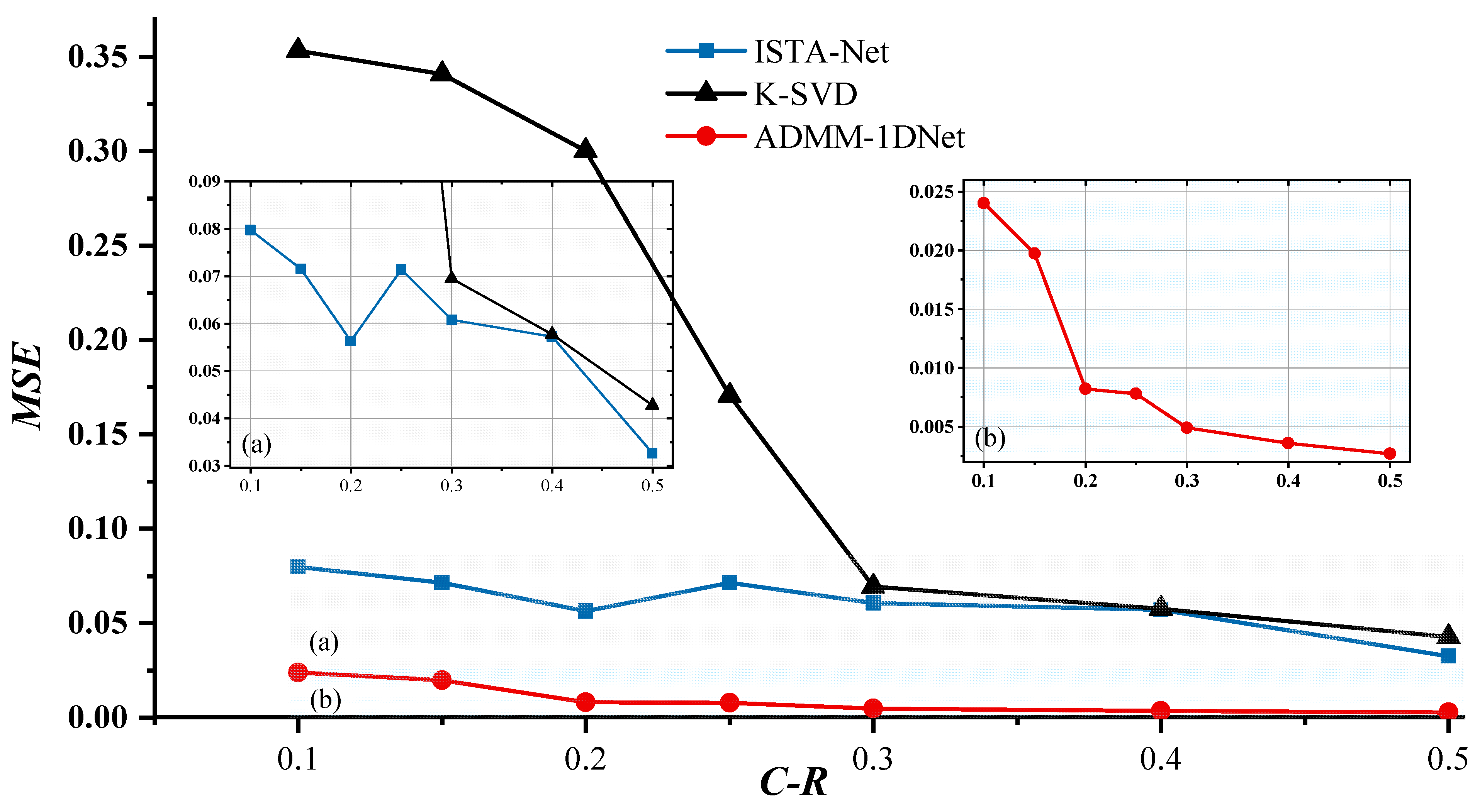
Figure 7 shows the relationship between L_S and T_test, and it can be observed that as the signal L_S increases, the T_test of the reconstructed signal of the three algorithms increases. It is noted that the reconstruction T_test of ADMM-1DNet at signal sparse levels of 0.2 and 0.3 is much lower than that of the other two algorithms, and the results remain relatively stable. This demonstrates that the ADMM-1DNet implementation scheme still has good robustness when processing signals with different sparse levels and can adapt to the task requirements of signal reconstruction with different sparse levels.

4.3. Real Signal Experiment

4.3.1. Experimental Data

Following the network parameter setting guidelines specified in Section 4.2.1, in the real bearing vibration signal, the reconstruction performance of the ISTA-Net network proposed in literature [48] and the ADMM + K-SVD-based CS method in literature [35] are compared with the ADMM-1DNet network algorithm proposed in this paper. To ensure the fairness of the algorithm reconstruction experiment, the parameters of the CS method based on ADMM + K-SVD are also optimized by the embedded program. The whole reconstruction process is described in Section 2.3.

Two authoritative bearing experimental data sets are used in the experiment: the bearing experimental data set (CWRU) [64], published by CASE Western Reserve University, and the bearing experimental data set (XJTU-SY) [65], published by Xi’an Jiaotong University. Figure 8 shows the test rigs and the bearings used for the two datasets. The CWRU vibration data was collected using accelerometers, which were attached to the housing with magnetic bases. Accelerometers were placed at the 12 o’clock position at both the drive end and fan end of the motor housing. Four types of bearing data at the drive end were selected as sample signals in the dataset with a signal frequency of 12 kHz, a motor load of 1 HP, and a fault diameter of 0.007″. In the XJTU-SY, two accelerometers of type PCB 352C33 are positioned at 90° on the housing of the tested bearings, i.e., one is mounted on the horizontal axis and the other is mounted on the vertical axis. In the dataset, the horizontal outer ring fault signal is selected as the sampling signal at 40 Hz, the signal sampling frequency is 25.6 kHz, and a total of 32,768 data points are recorded in each sampling, i.e., 1.28 s, with a sampling period of 1 min. In order to fully simulate the outdoor working environment of mechanical equipment, Gaussian white noise with an SNR of 30 dB is added to all signals.

Considering the limited number of equipment fault signal acquisitions, we expand the data set by sliding window sampling and take 1024 sampling points as a signal sample unit. Then, the training set and the test set for each signal are set to be 1200 and 240 sample units, respectively. The dataset name and fault type are shown in

Table 2. Dataset signal type and bearing parameters.

Dataset	Bearing Parameters					Signal Type
	Number of Balls (N)	Ball Diameter d/mm	Diameter D/mm	Contact Angle α/(°)	Rotational Speed (r/s)
CWRU	9	7.94	38.5	0	1772	Normal, IR, OR@6, BA
XJTU-SY	8	7.92	34.55	0	2400	MIX, IR, OR

. Normal represents the normal state; BA, OR, and IR, respectively, represent the ball, outer ring, and inner ring faults; and the number after @ represents the orientation of the fault point. MIX includes four kinds of mixed faults: inner ring, outer ring, rolling element, and cage.

4.3.2. Frequency Domain Quality Analysis of Reconstructed Signals

Whether the reconstructed signal can retain the characteristic frequency of the original signal is another important indicator to test the reconstruction performance of the algorithm. When a ball in the bearing rolls over the fault location, it will produce an instantaneous pulse, so the reciprocal of the time interval between any two adjacent pulses is the fault characteristic frequency, which is determined by the rotation frequency of the bearing and the nature of the fault type. In general, for angular contact ball bearings with fixed outer raceways and rotating inner raceways, the formulas [66,67] for the theoretical values of the Ball Passing Frequency Inner (BPFI) and Ball Passing Frequency Outer (BPFO) are (f_r is the rotational frequency) as follows:

$$f_{\mathrm{BPFI}}=\frac{N}{2}{f}_r\left(1+\frac{d}{D}\cos \alpha \right)$$

(35)

$$f_{\mathrm{BPFO}}=\frac{N}{2}{f}_r\left(1-\frac{d}{D}\cos \alpha \right)$$

(36)

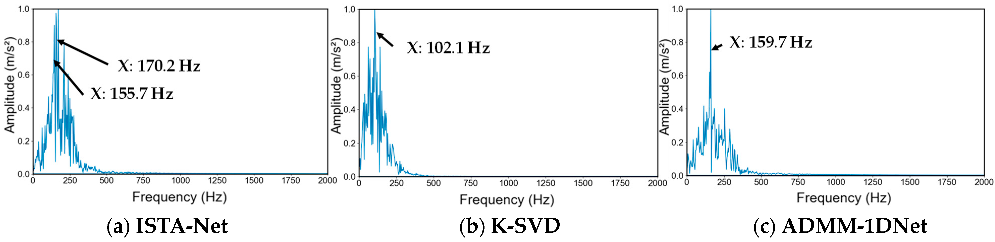
IR and OR fault signal data from the CWRU and XJTU-SY data sets are taken as experimental objects. Based on the calculation formula, the BPFI of the driving end-bearing signal in the CWRU data set is 160.3 Hz, and the BPFO is 105.5 Hz. The BPFI of the horizontal bearing signal in the XJTU-SY dataset is 196.7 Hz, and the BPFO is 123.3 Hz.

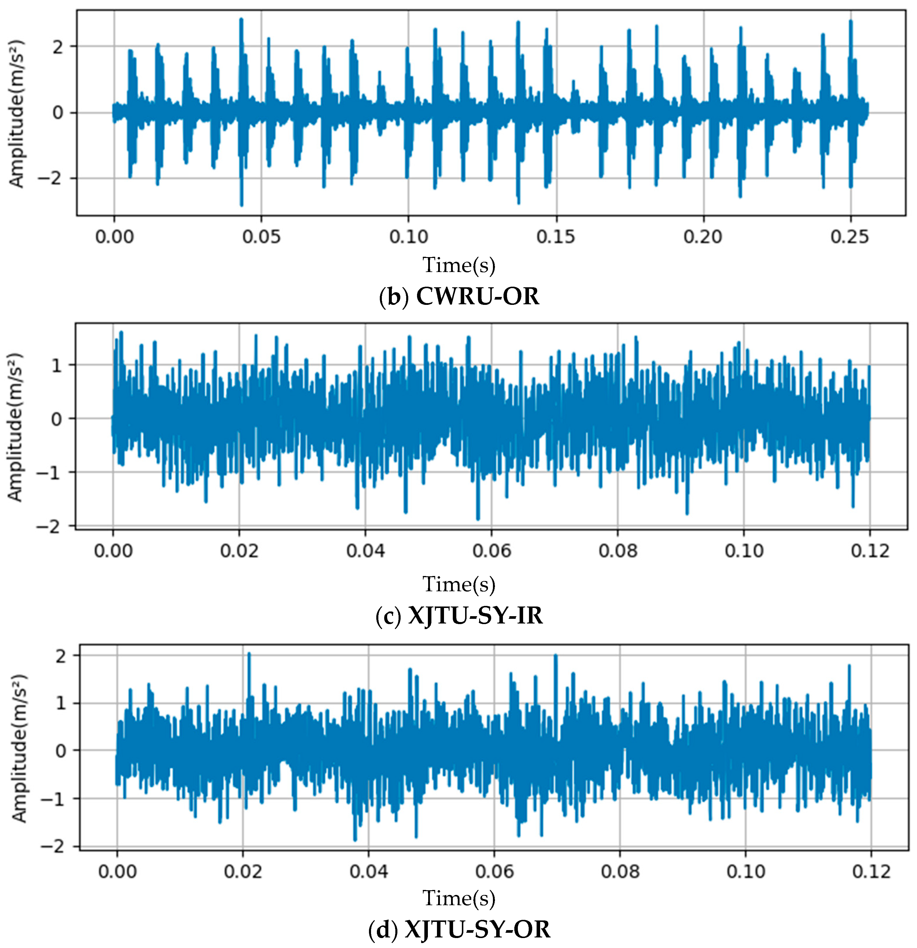
Considering the limited number of fault signals collected during equipment bursts, we selected 3072 sampling points from each signal after reconstruction for characterization. Figure 9a,b show the IR and OR fault signal time-domain waveforms of the CWRU dataset, and Figure 9c,d show the IR and OR fault signal time-domain waveforms of the XJTY-SY dataset. Using the ISTA-Net network, ADMM-1DNet network, and ADMM + K-SVD-based reconstruction algorithm to conduct reconstruction experiments on the above four signals and conduct empirical mode decomposition on the reconstructed signals to further analyze the signal composition and feature information.

By comparing Figure 10, Figure 11, Figure 12 and Figure 13, it is found that the reconstruction effect of the ADMM + K-SVD algorithm is the worst compared with the other two network-based algorithms, and the peak value displayed after empirical mode decom-position (EMD) is far from the theoretical value. These unwanted peaks can lead to a misinterpretation of part failure characteristics during fault diagnosis and classification. As shown in Figure 10a and Figure 13a, the reconstruction results of ISTA-Net detect the characteristic frequency of the approximate theoretical value, but there are other obvious frequency peaks near the approximate value. However, the corresponding characteristic frequencies of the four kinds of signals after reconstruction of ADMM-1DNet are close to the theoretical values, and the difference between them is not more than 0.6%, and no other approximate peak is found. The experimental results demonstrate that, compared with the other two baseline methods, the signal reconstructed by ADMM-1DNet can still retain relevant frequency and feature information under high noise and high r, which proves the effectiveness of the proposed online monitoring scheme for practical application purposes.

Table 3. Reconstructed signal indicator results.

Method	CWRU				XJTU-SY
	$\mathbf{I}\mathbf{R}-{\mathit{T}}_{\mathbf{test}}$	BPFI	$\mathbf{O}\mathbf{R}-{\mathit{T}}_{\mathbf{test}}$	BPFO	$\mathbf{I}\mathbf{R}-{\mathit{T}}_{\mathbf{test}}$	BPFI	$\mathbf{O}\mathbf{R}-{\mathit{T}}_{\mathbf{test}}$	BPFO
ISTA-Net	0.3977	170.2	0.3461	81.6	0.2824	223.7	0.3059	120.5
ADMM + K-SVD	0.2532	102.1	0.3046	148.2	0.4057	354.9	0.3961	79.5
ADMM-1DNet	0.0019	159.7	0.0081	105.3	0.0497	197.3	0.0675	123.1

records the specific T_test and characteristic frequency values of the above reconstruction results. The results were obtained by the algorithm through 100 iterations at most. It is found that the corresponding theoretical characteristic frequency values are detected no matter whether the reconstruction T_test is 0.0019 or 0.0675. We further visualize the experimental results corresponding to the above two accuracies. (The optimal reconstruction results of the experiments on the two datasets are selected here for visualization). Figure 14a shows the fitting diagram of the IR signal and reconstructed signal of the CWRU dataset, the T_test is 0.0019. Figure 14b shows the fitting diagram of the OR signal and reconstructed signal of the XJTU-SY dataset; the T_test is 0.0675. It can be observed that, compared with the OR signal, the IR signal has a lower T_test value, which means the latter has a higher fit accuracy than the original signal. However, the difference between the reconstructed signal and the original signal under the two accuracies is very small, almost completely coincident. This indicates that when the reconstructed T_test is lower than a certain value, the reconstructed signal has the most important feature information of the original signal, and the corresponding feature frequency can be displayed through empirical mode decomposition and other methods. Therefore, from the perspective of practical engineering applications, we believe that after a certain number of iterations, the iteration can be stopped when the signal has the corresponding characteristic frequency. While continuing iteration can improve reconstruction accuracy, it also slows down the convergence of the algorithm and increases the cost of unnecessary time.

4.3.3. Performance Analysis of Signal Reconfiguration Schemes

Signal reconstruction experiments were conducted by feeding the same compressed measurement signal y into the trained ISTA-Net, ADMM-1DNet, and ADMM + K-SVD algorithm methods. (For fairness, all reconstruction methods operate independently on the same computer by comparing the evaluation indexes in Section 4.1).

Figure 15a plots the time-frequency diagram of the CWRU dataset BA fault signal after noise addition, and Figure 16 shows the corresponding signal reconstruction results of the three algorithms at different compression rates. It can be observed that the ADMM-1DNet network can maintain an extremely low restructuring T_test even at 20% high r. The reconstruction T_test of the K-SVD method decreases with the increase in r, but the value is still much higher than that of the method proposed in this paper. The ISTA-Net network has unstable reconstruction results with increasing r; it has a lower T_test for reconstruction only at a certain r and is still numerically higher than the method proposed in this paper.

Table 4. Comparison of PSNR (dB), Time, and T_gen results for three algorithms reconstructing the BA signal of the CWRU dataset at different compression rates. The best performance is marked in bold, and the second-best performance is underlined. Time is a running time record for the three methods, showing the average time used for 100 iterations of 1024 samples.

C_R	ISTA-Net			ADMM + K-SVD			ADMM-1DNet
	PSNR (dB)	Time (S)	Tgen	PSNR (dB)	Time (S)	Tgen	PSNR (dB)	Time (S)	Tgen
10%	21.9046	1.7225	0.0107	17.9538	3.6527	--	27.6102	0.6467	0.00120
15%	22.3762	1.3144	0.0082	18.1029	3.6453	--	28.3691	0.7308	0.00175
20%	23.4711	1.2104	0.0056	18.2139	3.6291	--	31.4135	0.6708	0.00051
25%	22.5738	1.3024	0.0093	19.5731	3.5562	--	32.5003	0.6833	0.00048
30%	23.7329	1.3991	0.0053	22.5722	3.5421	--	33.0522	0.7117	0.00041
40%	24.8563	1.3667	0.0048	24.3601	3.5409	--	35.8264	0.7608	0.00022
50%	27.5307	1.2941	0.0041	25.4638	3.5527	--	36.6274	0.6717	0.00016

records the reconstructed PSNR and Time values. Under the same r, the ADMM-1DNet network achieves the highest PSNR value, and the algorithm has the fastest convergence speed, while other classical algorithms can only show high performance at a low compression rate. This demonstrates that the proposed network fully combines the advantages of the ADMM algorithm, deep neural network, and redundant analysis operator and significantly improves algorithm reconstruction accuracy and convergence speed.

The MIX fault signal of the XJTU-SY dataset with higher signal complexity is selected as the reconstruction object. Figure 15b plots its noise-adding time-frequency diagram. Figure 17 shows the reconstruction results of the three algorithms under different compression rates. It can be observed that when facing complex signals, the ISTA Net network is almost unable to complete reconstruction at compression rates of 25% and 30%, but the T_test of the ADMM-1DNet network is still significantly lower than the other two algorithms. In addition, the PSNR and Time values of the three algorithms under different compression rates are recorded in

Table 5. Comparison of PSNR (dB), Time, and T_gen results for three algorithms reconstructing the MIX signal of the XJTU-SY dataset at different compression rates. The best performance is marked in bold, and the second-best performance is underlined. Time is a running time record for the three methods, showing the average time used for 100 iterations of 1024 samples.

C_R	ISTA-Net			ADMM + K-SVD			ADMM-1DNet
	PSNR (dB)	Time (S)	Tgen	PSNR (dB)	Time (S)	Tgen	PSNR (dB)	Time (S)	Tgen
10%	18.1488	1.7350	0.0647	15.6798	3.7033	--	19.1659	0.7400	0.0150
15%	18.5336	1.9292	0.0586	15.2853	3.6672	--	20.3437	0.6841	0.0021
20%	19.0301	1.7533	0.0555	15.2113	3.6574	--	22.0323	0.7150	0.0036
25%	7.8792	1.7575	0.0953	17.0009	3.6502	--	23.3325	0.7058	0.0024
30%	8.8558	1.7358	0.1062	18.1672	3.5468	--	25.2719	0.7425	0.0017
40%	19.0870	1.7275	0.0124	20.6455	3.5397	--	26.1580	0.7217	0.0021
50%	16.6747	1.6250	0.0498	21.2260	3.5564	--	26.9997	0.7350	0.0011

. It can be seen that the ADMM-1DNet network has a high reconstruction accuracy, while the PSNR and Time (t) of the reconstructed signals are better than the baseline algorithms.

Table 4 and Table 5 also record their reconstruction T_gen values for two network algorithms involving testing and training. The results show that the T_gen between the two algorithms is almost one order of magnitude different, and the generalization of the ADMM-1DNet network is obviously superior to the ISTA-Net network. Excellent generalization means that the network can effectively process unfamiliar data without being limited to a specific data set or signal type, which is more robust and reliable in practical applications.

5. Conclusions

In this paper, a new CS signal reconstruction method based on ADMM and neural networks, called ADMM-1DNet, is especially suitable for the demand for online monitoring of devices in outdoor high-noise environmental conditions. Taking bearing parts as an example, combined with modern sensor technology, a detailed implementation scheme for monitoring mechanical equipment parts is given in this paper. Through experiments on simulated signals and real bearing vibration signals, we first formulate the parameter setting guidelines for the ADMM-1DNet network, then explore the relationship between the signal sparsity level and the reconstruction error, and finally examine the time-frequency domain quality of the reconstruction signals in a real data set. The experiments show that the proposed network outperforms other classical algorithms in terms of reconstruction accuracy and convergence speed, while the learning of redundant analysis operators enables the online monitoring scheme to adapt to signals with different sparsity levels, which can further satisfy the needs of different reconstruction tasks. The method in this paper provides strong theoretical and practical scheme support for practical engineering applications and is expected to play an important role in the field of monitoring parts of outdoor working machinery and equipment. In future work, we expect to develop a more powerful equipment monitoring system by fusing multimodal data on the basis of ADMM-1DNet to provide more comprehensive and reliable information for monitoring signal fault identification.

References

- Zhang, M.Q.; Zhang, H.X.; Zhang, C.T.; Yuan, D. Communication-efficient quantized deep compressed sensing for edge-cloud collaborative industrial IoT networks. IEEE Trans. Industr. Inform. 2022, 19, 6613–6623. [Google Scholar] [CrossRef]
- Plakias, S.; Boutalis, Y.S. A novel information processing method based on an ensemble of Auto-Encoders for unsupervised fault detection. Comput. Ind. 2022, 142, 103743. [Google Scholar] [CrossRef]
- Donoho, D.L. Compressed sensing. IEEE Trans. Inf. Theory 2006, 52, 1289–1306. [Google Scholar] [CrossRef]
- Landau, H.J. Sampling, data transmission, and the Nyquist rate. Proc. IEEE Inst. Electr. Electron. Eng. 1967, 55, 1701–1706. [Google Scholar] [CrossRef]
- Candès, E.J.; Wakin, M.B. An introduction to compressive sampling. IEEE Signal Process. Mag. 2008, 25, 21–30. [Google Scholar] [CrossRef]
- Haupt, J.; Nowak, R. Signal reconstruction from noisy random projections. IEEE Trans. Inf. Theory 2006, 52, 4036–4048. [Google Scholar] [CrossRef]
- Sarvotham, S.; Baron, D.; Wakin, M.; Duarte, M.F.; Baraniuk, R.G. Distributed compressed sensing of jointly sparse signals. In Proceedings of the Asilomar Conference on Signals, Systems and Computers, Pacific Grove, CA, USA, 30 October–2 November 2005; pp. 1537–1541. [Google Scholar]
- Wang, X.Y.; Liu, C.; Jiang, D.H. An efficient double-image encryption and hiding algorithm using a newly designed chaotic system and parallel compressive sensing. Inform. Sci. 2022, 610, 300–325. [Google Scholar] [CrossRef]
- Jiang, Y.Y.; Li, G.G.; Ge, H.Y.; Wang, F.; Li, L.; Chen, X.; Lv, M.; Zhang, Y. Adaptive compressed sensing algorithm for terahertz spectral image reconstruction based on residual learning. Spectrochim. Acta Part A Mol. Biomol. Spectrosc. 2022, 281, 121586. [Google Scholar] [CrossRef]
- Ma, H.M.; Yuan, X.J.; Ding, Z.; Fan, D.; Fang, J. Over-the-air federated multi-task learning via model sparsification, random compression, and turbo compressed sensing. IEEE Trans. Wirel. Commun. 2022, 22, 4974–4988. [Google Scholar] [CrossRef]
- Liang, L.K.; Shi, Y.R.; Shi, Y.W.; Bai, Z.; He, W. Two-dimensional DOA estimation method of acoustic vector sensor array based on sparse recovery. Digint. Signal Process. 2022, 120, 103294. [Google Scholar] [CrossRef]
- Wang, J.J.; Ren, L.; Jia, Z.; Jiang, T.; Wang, G.-X. A novel pipeline leak detection and localization method based on the FBG pipe-fixture sensor array and compressed sensing theory. Mech. Syst. Signal Process. 2022, 169, 108669. [Google Scholar] [CrossRef]
- Liu, C.; Wu, X.; Mao, J.L.; Liu, X. Acoustic emission signal processing for rolling bearing running state assessment using compressive sensing. Mech. Syst. Signal Process. 2017, 91, 395–406. [Google Scholar] [CrossRef]
- Tang, X.L.; Xu, Y.D.; Sun, X.Q.; Liu, Y.; Jia, Y.; Gu, F.; Ball, A.D. Intelligent fault diagnosis of helical gearboxes with compressive sensing based non-contact measurements. ISA Trans. 2023, 133, 559–574. [Google Scholar] [CrossRef]
- Guo, Y.N.; Li, B.W.; Yin, X. Dual-compressed photoacoustic single-pixel imaging. Natl. Sci. Rev. 2023, 10, nwac058. [Google Scholar] [CrossRef]
- Li, J.; Meng, Z.; Yin, N.; Pan, Z.; Cao, L.; Fan, F. Multi-source feature extraction of rolling bearing compression measurement signal based on independent component analysis. Measurement 2021, 172, 108908. [Google Scholar] [CrossRef]
- Dong, G.S.; Wan, H.P.; Luo, Y.Z.; Todd, M.D. A fast sparsity-free compressive sensing approach for vibration data reconstruction using deep convolutional GAN. Mech. Syst. Signal Process. 2023, 188, 109937. [Google Scholar] [CrossRef]
- Yuan, H.; Lu, C. Rolling bearing fault diagnosis under fluctuant conditions based on compressed sensing. Struct. Control Health Monit. 2017, 24, e1918. [Google Scholar] [CrossRef]
- Ganesan, V.; Das, T.; Rahnavard, N.; Kauffman, J.L. Vibration-based monitoring and diagnostics using compressive sensing. J. Sound Vib. 2017, 394, 612–630. [Google Scholar] [CrossRef]
- Perepu, S.K.; Tangirala, A.K. Reconstruction of missing data using compressed sensing techniques with adaptive dictionary. J. Process. Cont. 2016, 47, 175–190. [Google Scholar] [CrossRef]
- Bairi, Z.; Ben-Ahmed, O.; Amamra, A.; Bradai, A.; Bey, K.B. PSCS-Net: Perception optimized image reconstruction network for autonomous driving systems. IEEE Trans. Intell. Transp. 2022, 24, 1564–1579. [Google Scholar] [CrossRef]
- Li, H.D.; Ai, D.M.; Zhu, H.P.; Luo, H. Compressed sensing–based electromechanical admittance data loss recovery for concrete structural health monitoring. Struct. Health Monit. 2021, 20, 1247–1273. [Google Scholar] [CrossRef]
- Wang, H.K.; Li, Z.A.; Hou, X.S. Versatile denoising-based approximate message passing for compressive sensing. IEEE T Image Process. 2023, 32, 2761–2775. [Google Scholar] [CrossRef]
- Metzler, C.A.; Maleki, A.; Baraniuk, R.G. From denoising to compressed sensing. IEEE Trans. Inf. Theory 2016, 62, 5117–5144. [Google Scholar] [CrossRef]
- Dong, W.S.; Shi, G.G.; Li, X.; Ma, Y.; Huang, F. Compressive sensing via nonlocal low-rank regularization. IEEE Trans. Image Process. 2014, 23, 3618–3632. [Google Scholar] [CrossRef] [PubMed]
- Deng, L.F.; Lin, H.B.; Liu, Z.Z.; Wang, H. Compressed feature reconstruction for localized fault diagnosis with generalized minimax-concave penalty. Measurement 2022, 200, 111622. [Google Scholar] [CrossRef]
- Song, S.Z.; Zhang, X.; Hao, Q.S.; Wang, Y.; Feng, N.; Shen, Y. An improved reconstruction method based on auto-adjustable step size sparsity adaptive matching pursuit and adaptive modular dictionary update for acoustic emission signals of rails. Measurement 2022, 189, 110650. [Google Scholar] [CrossRef]
- Theis, F.J.; Jung, A.; Puntonet, C.G.; Lang, E.W. Signal recovery from partial information via orthogonal matching pursuit. IEEE Trans. Inform. Theory 2007, 53, 4655–4666. [Google Scholar]
- Donoho, D.L.; Tsaig, Y.; Drori, I.; Starck, J.L. Sparse solution of underdetermined systems of linear equations by stagewise orthogonal matching pursuit. IEEE Trans. Inf. Theory 2012, 58, 1094–1121. [Google Scholar] [CrossRef]
- Blumensath, T.; Davies, M.E. Iterative hard thresholding for compressed sensing. Appl. Comput. Harmon. A 2009, 27, 265–274. [Google Scholar] [CrossRef]
- Sabor, N. Gradient immune-based sparse signal reconstruction algorithm for compressive sensing. Appl. Soft. Comput. 2020, 88, 106032. [Google Scholar] [CrossRef]
- Li, J.E.; Tao, J.X.; Ding, W.M.; Zhang, J.; Meng, Z. Period-assisted adaptive parameterized wavelet dictionary and its sparse representation for periodic transient features of rolling bearing faults. Mech. Syst. Signal Process. 2022, 169, 108796. [Google Scholar] [CrossRef]
- Wang, X.; Zhang, S.N.; Zhu, L.Z.; Chen, S.; Zhao, H. Research on anti-narrowband am jamming of ultra-wideband impulse radio detection radar based on improved singular spectrum analysis. Measurement 2022, 188, 110386. [Google Scholar] [CrossRef]
- Lu, Y.L.; Wang, Y. A physics-constrained dictionary learning approach for compression of vibration signals. Mech. Syst. Signal Process. 2020, 153, 107434. [Google Scholar] [CrossRef]
- Anaraki, F.P.; Hughes, S.M. Compressive K-SVD. In Proceedings of the International Conference on Acoustics, Speech and Signal Processing, Vancouver, BC, USA, 26–31 May 2013; pp. 5469–5473. [Google Scholar]
- Baraniuk, R.; Davenport, M.; Devore, R.; Wakin, M. A simple proof of the restricted isometry property for random matrices. Constr. Approx. 2008, 28, 253–263. [Google Scholar] [CrossRef]
- Huang, Y.; Beck, J.L.; Wu, S.; Li, H. Bayesian compressive sensing for approximately sparse signals and application to structural health monitoring signals for data loss recovery. Probabilist. Eng. Mech. 2016, 46, 62–79. [Google Scholar] [CrossRef]
- Rani, M.; Dhok, S.B.; Deshmukh, R.B. A systematic review of compressive sensing: Concepts, implementations and applications. IEEE Access 2018, 6, 4875–4894. [Google Scholar] [CrossRef]
- Mascareñas, D.; Cattaneo, A.; Theiler, J.; Farrar, C. Compressed sensing techniques for detecting damage in structures. Struct. Health Monit. 2013, 12, 325–338. [Google Scholar] [CrossRef]
- Yao, H.T.; Dai, F.; Zhang, D.M.; Ma, Y.; Zhang, S.; Zhang, Y.; Tian, Q. DR2-Net: Deep residual reconstruction network for image compressive sensing. Neurocomputing 2019, 395, 483–493. [Google Scholar] [CrossRef]
- Mousavi, A.; Baraniuk, R.G. Learning to invert: Signal recovery via Deep Convolutional Networks. In Proceedings of the International Conference on Acoustics, Speech and Signal Processing, New Orleans, LA, USA, 5–9 March 2017; pp. 2272–2276. [Google Scholar]
- Shi, W.Z.; Feng, J.; Liu, S.H.; Zhao, D.B. Image compressed sensing using convolutional neural network. Trans. Image Process. 2020, 29, 375–388. [Google Scholar] [CrossRef] [PubMed]
- Gregor, K.; LeCun, Y. Learning fast approximations of sparse coding. In Proceedings of the 27th International Conference on Machine Learning, Haifa, Israel, 21–24 June 2010; pp. 399–406. [Google Scholar]
- Beck, A.; Teboulle, M. A fast Iterative Shrinkage-Thresholding Algorithm with application to wavelet-based image deblurring. In Proceedings of the 2009 IEEE ICASSP, Taipei, Taiwan, 19–24 April 2009; pp. 693–696. [Google Scholar]
- Ben Sahel, Y.; Bryan, J.P.; Cleary, B.; Farhi, S.L.; Eldar, Y.C. Deep unrolled recovery in sparse biological imaging: Achieving fast, accurate results. IEEE Signal Process. Mag. 2022, 39, 45–57. [Google Scholar] [CrossRef]
- Gadjimuradov, F.; Benkert, T.; Nickel, M.D.; Maier, A. Robust partial fourier reconstruction for diffusion-weighted imaging using a recurrent convolutional neural network. Magn. Reson. Med. 2021, 87, 2018–2033. [Google Scholar] [CrossRef] [PubMed]
- Barranca, V.J. Neural network learning of improved compressive sensing sampling and receptive field structure. Neurocomputing 2021, 455, 368–378. [Google Scholar] [CrossRef]
- Zhang, J.; Ghanem, B. ISTA-Net: Interpretable optimization-inspired deep network for image compressive sensing. In Proceedings of the IEEE CVPR, Salt Lake City, UT, USA, 18–22 June 2018; pp. 1828–1837. [Google Scholar]
- Ramírez, J.M.; Torre, J.I.M.; Fuentes, H.A. LADMM-Net: An unrolled deep network for spectral image fusion from compressive data. Signal Process. Recognit. 2021, 189, 108239. [Google Scholar] [CrossRef]
- Zhang, Z.H.; Liu, Y.P.; Liu, J.N.; Wen, F.; Zhu, C. AMP-Net: Denoising-based deep unfolding for compressive image sensing. IEEE Trans. Image Process. 2020, 30, 1487–1500. [Google Scholar] [CrossRef] [PubMed]
- Machidon, A.L.; Pejović, V. Deep learning for compressive sensing: A ubiquitous systems perspective. Artif. Intell. Rev. 2023, 56, 3619–3658. [Google Scholar] [CrossRef]
- Wang, X.C.; Li, J.; Wang, D.P.; Huang, X.; Liang, L.; Tang, Z.; Fan, Z.; Liu, Y. Sparse ultrasonic guided wave imaging with compressive sensing and deep learning. Mech. Syst. Signal Process. 2022, 178, 109346. [Google Scholar] [CrossRef]
- Yin, Z.; Shi, W.Z.; Wu, Z.C.; Zhang, J. Multilevel wavelet-based hierarchical networks for image compressed sensing. Pattern Recogn. 2022, 129, 108758. [Google Scholar] [CrossRef]
- Boyd, S.; Parikh, N.; Chu, E.; Peleato, B.; Eckstein, J. Distributed optimization and statistical learning via the alternating direction method of multipliers. Found. Trends Mach. Le. 2010, 3, 1–122. [Google Scholar] [CrossRef]
- Narwaria, M. Does explainable machine learning uncover the black box in vision applications? Image Vision Comput. 2022, 118, 104353. [Google Scholar] [CrossRef]
- Zhao, L.J.; Wang, X.L.; Zhang, J.J.; Wang, A.; Bai, H. Boundary-constrained interpretable image reconstruction network for deep compressive sensing. Knowl. Based Syst. 2023, 275, 110681. [Google Scholar] [CrossRef]
- Lin, H.B.; Tang, J.M.; Mechefske, C. Impulse detection using a shift-invariant dictionary and multiple compressions. J. Sound Vib. 2019, 449, 1–17. [Google Scholar] [CrossRef]
- Chen, X.F.; Du, Z.H.; Li, J.M.; Li, X.; Zhang, H. Compressed sensing based on dictionary learning for extracting impulse components. Signal Process. 2014, 96, 94–109. [Google Scholar] [CrossRef]
- Li, L.X.; Fang, Y.; Liu, L.; Peng, H.; Kurths, J.; Yang, Y. Overview of compressed sensing: Sensing model, reconstruction algorithm, and its applications. Appl. Sci. 2020, 10, 5909. [Google Scholar] [CrossRef]
- Treskatis, T.; Moyers-González, M.A.; Price, C.J. An accelerated dual proximal gradient method for applications in viscoplasticity. J. Non-Newton Fluid 2016, 238, 115–130. [Google Scholar] [CrossRef]
- Li, P.C.; Ding, Z.G.; Zhang, T.Y.; Wei, Y.; Gao, Y. Integrated detection and Imaging algorithm for radar sparse targets via CFAR-ADMM. IEEE Trans. Geosci. Remote 2023, 61, 1–15. [Google Scholar] [CrossRef]
- Ghahremani, M.; Liu, Y.H.; Yuen, P.; Behera, A. Remote sensing image fusion via compressive sensing. ISPRS J. Photogramm. 2019, 152, 34–48. [Google Scholar] [CrossRef]
- Haneche, H.; Boudraa, B.; Ouahabi, A. A new way to enhance speech signal based on compressed sensing. Measurement 2020, 151, 107117. [Google Scholar] [CrossRef]
- Loparo, K. Case western reserve university bearing data center. In Bearings Vibration Data Sets; Case Western Reserve University: Cleveland, OH, USA, 2012; pp. 22–28. [Google Scholar]
- Wang, B.; Lei, Y.G.; Li, N.P.; Li, N. A hybrid prognostics approach for estimating remaining useful life of rolling element bearings. IEEE Trans. Reliab. 2018, 69, 401–412. [Google Scholar] [CrossRef]
- Smith, W.A.; Randall, R.B. Rolling element bearing diagnostics using the Case Western Reserve University data: A benchmark study. Mech. Syst. Signal Process. 2015, 64, 100–131. [Google Scholar] [CrossRef]
- Yuwono, M.; Qin, Y.; Zhou, J.; Guo, Y.; Celler, B.G.; Su, S.W. Automatic bearing fault diagnosis using particle swarm clustering and Hidden Markov Model. Eng. Appl. Artif. Intel. 2016, 47, 88–100. [Google Scholar] [CrossRef]