
Enhancing Renewable Energy Accommodation by Coupling Integration Optimization with Flexible Retrofitted Thermal Power Plant
State Key Laboratory of Power Transmission Equipment Technology, School of Electrical Engineering, Chongqing University, Chongqing 400044, China
*
Author to whom correspondence should be addressed.
Appl. Sci. 2024, 14(7), 2907; https://doi.org/10.3390/app14072907
Submission received: 12 March 2024
/
Revised: 24 March 2024
/
Accepted: 28 March 2024
/
Published: 29 March 2024
(This article belongs to the Special Issue Advanced Technologies and Applications of Microgrids)
Abstract
:Featured Application
The proposed method in this paper can be utilized to assess the enhanced accommodation capability of renewable energy sources following the coupling integration with retrofitted thermal power units.
Abstract
Thermal power units (TPUs) play a crucial role in accommodating the high penetration of renewable energy sources (RESs) like wind turbines (WTs) and photovoltaics (PVs). This paper proposes an evaluation framework to quantitatively analyze the flexibility potential of retrofitted TPUs in enhancing the accommodate capability of RESs through coupling integration and optimal scheduling. Firstly, the coordination framework for coupling TPUs with RESs is outlined, including a comprehensive analysis of benefits and implementation strategies. Secondly, an annual optimal scheduling model for TPUs and RESs is developed, incorporating deep peak regulation services, ladder-type constraints for retrofitted TPUs, and their operational characteristics before and after the coupling integration. Thirdly, indices to evaluate RES accommodation levels and TPU regulation capacities are proposed to quantify the performance of power sources. Finally, a real-world case study is conducted to demonstrate that integrating retrofitted TPUs with RESs through coupling significantly enhances RES utilization by 3.6% and boosts TPUs’ downward regulation capabilities by 32%.
1. Introduction
In the face of escalating concerns over environmental pollution, global warming, and energy security, power systems worldwide are evolving towards a higher penetration of renewable energy sources (RESs) [1]. However, the inherent variability and intermittency of RESs, such as wind turbines (WTs) and photovoltaic (PV) generation, pose significant challenges to their integration [2]. Efficiently accommodating these fluctuations within the existing power grid infrastructure is a critical challenge that needs to be addressed. With the continued growth in the installed capacity of RESs, there is an urgent need for a more flexible power system that would maximize the economic and environmental benefits of clean energy [3].
To achieve effective RES utilization, it is essential to leverage the flexibility support from conventional power sources on the generation side. In areas predominantly reliant on coal, thermal power units (TPUs) act as the main providers of power system flexibility [4]. Enhancing the flexibility of TPUs through technical retrofitting emerges as the most realistic and feasible method to augment the power system’s adaptability [5]. By implementing measures like optimizing auxiliary combustion and steam-water processes, TPUs can enhance their ramping efficiency and operate below the minimum output of a regular peak regulation (RPR) state, thereby achieving deep peak regulation (DPR) capabilities [6,7]. This enables TPUs to provide a greater regulation capacity, fostering better RES utilization and obtaining additional revenues from auxiliary services [8].
To assess RES accommodation capabilities through flexible power sources like TPUs, the authors of [9] evaluated the capabilities of existing coal-fired power plants in Germany to integrate different shares of RESs based on historical operation data. Reference [10] assessed the technical and economic performance of the main flexible resources for RES accommodation based on the Beijing–Tianjin–Hebei region in China. Reference [11] assessed the flexibility requirements, including the maximum ramping rate and minimum output for TPUs, to accommodate future large-scale variable RESs. These studies focused on conducting a macro-level evaluation of the RES accommodation capability of flexible resources across broad regions but failed to precisely explore and utilize the potential flexibility of retrofitted TPUs.
The optimization and coordination between TPUs and RESs are important ways to schedule the TPUs at the time-step level to improve the accommodation of RESs. In [12], a stochastic rolling economic dispatch was developed to explore the benefits of retrofitted TPUs in wind-integrated power systems. In [13], an appropriate look-ahead scheduling framework for a wind–thermal power system considering the retrofitted coal-fired TPUs and the flexible load transfer strategy was proposed to smooth power fluctuations with an economic dispatch. In [14], an optimal scheduling model for TPUs and WTs considering the cost of DPR was proposed to minimize the total cost by searching for the optimal wind power curtailment. In [15], a nondominated-sorting grey wolf optimizer algorithm for the multi-objective load dispatch of TPUs and RESs with the consideration of efficient nondominated sorting was proposed. In [16], a dispatching model based on RES forecasting errors was proposed for wind–PV–thermal-coordinated operations. In [17], a multi-technical flexibility retrofit planning model of TPUs was developed to reduce the total cost and increase the accommodation of stochastic wind power within the power grid.
The coordination of TPUs and RESs discussed above is primarily based on power systems that may encompass long electrical distances and grid structures between power sources with a potentially complicated power-flow distribution. Such power-flow constraints in the coordinated operation may hinder the full utilization of the flexibility offered by retrofitted TPUs. To address this challenge, a feasible solution is the coupling integration of RESs and TPUs at a close physical distance, which are connected to the main power grid at the point of common coupling (PCC). This form of coordination operates as an integrated coupling generation system (CGS) for better coordination without considering the grid structure [18]. The CGS can more efficiently utilize the flexibility of TPUs to participate in DPR auxiliary services and accommodate RESs. Research in [19] demonstrates that the TPUs in CGS can achieve a real-time frequency response to handle the dynamic operation states of RESs. In [20], the coupling effect of TPUs and RESs was analyzed to demonstrate that CGS can achieve better coordination between power sources. In [21], an optimal scheduling strategy that fully considers the contributions of WT farms, PV parks, and TPUs to determine economic benefits and an environmental impact equilibrium in a hybrid generation system under natural limitations was proposed. In [22], a day-ahead optimal dispatch model of the coupled system was established based on the operation characteristics of DPR auxiliary services and the ladder-type ramping of TPUs. In [23], an optimal scheduling approach of CGS was presented to demonstrate that coupling integration can improve the economic benefits of the system. The above CGS studies have predominantly concentrated on the economic benefits facilitated by coupling integration, overlooking the quantitative evaluation of enhancements in RES utilization after coupling integration compared to the scenario before coupling. Moreover, there has been limited attention to the detailed implementation scheme for the real-world CGS with TPUs and RESs.
To sum up, previous studies [9,10,11] that conducted macroscopic evaluations on the impact of retrofitted TPUs for improving the accommodation capability of RES did not fully exploit their potential for detailed coordination at the time-step level. On the other hand, the optimal scheduling models for TPUs and RESs in previous studies [12,13,14,15,16,17,18,19,20,21,22,23] lack the ability to quantitatively measure the improvements in RES accommodation of different coordination methods with TPUs. To address the aforementioned gaps, this paper proposes an evaluation framework to assess the enhanced accommodation capabilities of RESs following the coupling integration optimization of retrofitted TPUs with WT and PV. Firstly, the analysis of the flexibility of TPUs, the accommodation measures of RESs, and the coordination framework of coupling integration for TPUs and RESs is presented. The implementation strategy for integrating the power sources into CGS is given in detail. Based on the above, an optimal power-source scheduling model is established based on the operation characteristics before and after retrofitting, as well as the features of DPR services. Then, the indices for assessing the RES accommodation level and TPU regulation marginals are proposed to quantify the performance of power sources before and after coupling and retrofitting. Finally, through a real-world project, the effectiveness of the proposed method is validated, demonstrating that retrofitted TPUs in CGS can improve the system’s regulation marginals while maximizing the accommodation of RESs.
2. Coupling Coordination Framework
2.1. Basic Framework
TPUs play a crucial role in providing flexibilities for RESs like WT and PV in regions with insufficient flexible regulatory resources. Traditionally, in the power grid’s operational framework, TPUs, WT farms, and PV plants operate as standalone entities [12]. The main power grid’s operator sends dispatch instructions to these various energy sources independently. As depicted in Figure 1a, the dispatch instructions to TPUs are given based on forecasted outputs from the RES and load demand. Under this scenario, TPUs lack the capability to monitor and accommodate the real-time energy production from RESs; thus, the flexibility potential of TPUs cannot be fully utilized. The complex network structure and operational limitations within the large power grid mean that only a fraction of the RES fluctuations can be mitigated by the grid’s flexibility. Consequently, any RES generation exceeding this capacity will be discarded, leading to inefficient utilization.
To address the above issues, a CGS that aggregates the RESs and TPUs into an integrated control object and operating entity connected to the main power grid at the same point of common public (PCC) is a feasible and effective solution. In this scenario, both the physical distance and electrical connections of RESs and TPUs are close. Hence, the RESs and TPUs can be dispatched by the power grid as an integrated singular unit. As depicted in Figure 1b, the CGS coordinates the output of the internal power sources based on the dispatching instructions received from the main power grid operator. The instruction specifies the power required to be generated by the CGS during a time period; it is typically related to the load demand and RES output. To effectively manage the fluctuations associated with a high penetration of RESs within the CGS, TPUs typically undergo technological upgrades. These enhancements are aimed at increasing their ramping capabilities and expanding the output range.
2.2. Benefit Analysis and Implementation Measures
Compared to the similar concepts of a BRTGS and VPP, a CGS represents a unique approach that integrates multiple power sources with distinctive characteristics. A BRTGS mainly concentrates on the direct transmission of RESs with TPUs across different regions through high-voltage AC/DC transmission lines. The transmission power in BRTGSs is relatively stable, with infrequent variations. Additionally, they do not prioritize the geographical proximity of the power sources. On the other hand, a VPP emphasizes coordinating Distributed Energy Resources (DERs) like energy storage, controllable loads, and electric vehicles on the demand side to facilitate flexible regulation. A VPP’s focus is predominantly on managing demand rather than supply, and the connected DERs are usually distributed across the grid. The distinctions between CGSs, BRTGSs, and VPPs are shown in Table 1; the table highlights the distinct objectives, coordination methods, and functional roles of CGSs, BRTGSs, and VPPs.
Compared with the independent operation of RESs and TPUs, a CGS unifies geographically proximate power sources within the power grid. Through efficient internal coordination, the CGS operates as an integrated singular unit, supplying power to the main grid. The key advantages of CGSs include
- Enhanced accommodation of RES fluctuations: A CGS allows for more effective handling of the inherent fluctuations in RES generation through its internal retrofitted TPUs without the need to consider the intricacies of the power flow or rely on coordination between operators across different regions.
- Seamless integration into existing infrastructure: Qualified power sources can be effortlessly aggregated as CGSs use the existing power grid structure. This facilitates a broad adoption with minimal investment requirements for power-source operators. For instance, in the power grid of Liaoning, China, the capacity of RESs and TPUs that can be interconnected at the same PCC exceeds 42% [22].
- Simplified dispatch within the main power grid: Acting as a unified dispatch entity, CGSs can integrate smoothly with the prevailing main power grid. They simplify the scheduling process for the main power grid operator by eliminating the need for the comprehensive modeling of each power source within the CGS. Furthermore, dispatching instructions from the main power grid can be determined without extensive consideration for accommodating fluctuations from RESs.
- Decentralized scheduling with high efficiency: The power source scheduling can be divided between the main power grid and CGS levels, significantly easing the modeling and computational complexity.
- Enhanced revenue generation from the auxiliary service market: With precise control mechanisms, the TPUs within the CGS can more effectively participate in the DPR auxiliary service. This participation not only fully exploits the operational flexibility of retrofitted TPUs but also boosts the overall economic benefits of the whole CGS.
The integration of power sources into the CGS in practical engineering applications can be smoothly accomplished. It necessitates the creation of a coordinated control and optimization management center. This center can be located either at the power sources or hosted on a cloud server by a reliable third party. Its core role is to facilitate coordinated optimization and control of the power sources within the CGS, taking into account dispatching instructions from the main power grid and status data from internal power sources. Furthermore, it is essential to install rapid response control systems and status monitoring equipment at TPU and RES plants. These installations are crucial for executing control instructions from the coordination center and providing vital information regarding the status of the power sources, such as the current output and resource utilization. With these measures in place, the CGS can achieve effective internal coordination of the power sources. Specifically, TPUs within the CGS can employ their rapid response devices to fully leverage their flexibility in response to real-time fluctuations of RESs, thereby accommodating more RES generation.
3. Model Development
In this section, to comprehensively evaluate the overall RES accommodation level under different seasons, an optimal dispatching model for WTs, PV, and TPUs before and after coupling integration based on the annual RES outputs and load demands (i.e., dispatching instructions) data is established. The time scale of the optimization is based on a 30 min time interval, which is widely used for power source scheduling [24]. The model is designed to evaluate the impact of technologically retrofitted TPUs with increased flexibility for improving the accommodation of RESs through coupling integration. To facilitate the solution process, the Big-M method is employed to relax the constraints. Following this, the methodology for assessing the accommodation capability of RESs is detailed. In this section, unless stated otherwise, the unit of power is measured in megawatts (MW), while both revenues and costs are expressed in Chinese Yuan (CNY).
3.1. Objective Function
From the perspective of CGS operators, their operation goal is to achieve the economic operation of the system. Therefore, the objective function is formulated to maximize total annual revenues, taking into account the generation of revenue from each power source, revenue from DPR auxiliary service revenue, operational costs, and pollution emission costs. The objective function is presented as follows:
In (1), is the total generation revenue of TPUs; it is related to the real-time DPR service they can provide at a time step [25]
The function of Equation (4) serves to calculate the revenue that a startup TPU can obtain. comprises basic revenue and DPR service revenue. The basic revenue corresponds to , and the unit price is . The first line in the equation represents DPR service revenue only, which can be obtained when the output rate of a TPU is lower than the compensation standard . The second line of the equation indicates that the current active output of TPU can obtain additional first-tier DPR service revenue with a unit price of . This revenue is calculated based on the difference between the active output corresponding to the compensation standard and the current active output . The third line of Equation (4) represents the current active output of TPU, which is lower than the compensation standard , and can obtain second-tier DPR service revenue. The calculation method remains consistent with the first tier, except that the unit price changes to .
is the operation cost of the startup TPUs, encompassing coal consumption, maintenance expenses, and extra costs associated with the DPR state [26].
where , denote that the TPU is operating in the RPR state; conversely, absence of these conditions indicates the opposite.
In Equation (6) ①, when the TPU is in the RPR state (i.e., the active output is greater than ), adopts the commonly used coal consumption cost-fitting function [27]. In Equation (6) ②, when the TPU operates in the DPR state (i.e., the active output is below ), an additional cost is incurred to sustain the TPU’s operation under low-output conditions calculated with the fitting function [28].
is the startup cost of TPUs
is the pollution treatment cost of TPUs [29]
In this study, smoke, SO2, and NOx are considered.
and are the generation revenues of WT and PV
represents the penalty incurred for inadequate power generation within the CGS that does not satisfy the load demand
where .
3.2. Constraints
The constraints take into account the power balance constraints, power-source output constraints, flexible constraints of TPUs, and ramping constraints of TPUs.
To accurately describe the scheduling characteristics of power sources before and after the coupling integration of retrofitted TPUs with RESs, this paper establishes the following two power balance constraints:
(a) Before implementing coupling integration (independent operation), the main power grid dispatches separate instructions to different power sources. For TPUs, the dispatch instructions are based on the forecasted net load, which is calculated as the forecast load demand minus the forecast outputs of WT and PV. The dispatch instructions for WT and PV are derived from their predicted outputs. The flexibility of TPUs is solely employed to mitigate minor fluctuations based on the dispatch instructions without addressing the variability from WT and PV outputs. Fluctuations from WT and PV are partially absorbed by the main power grid. Any excess generation from WT and PV that cannot be accommodated results in curtailment. Given these settings, the power balance constraints disregarding the integration are as follows:
where and represents the upper and lower limits of the main power grid’s capability to accommodate fluctuations from RESs. Due to limitations imposed by power-flow constraints and insufficient information, power sources within the main grid often struggle to coordinate efficiently without coupling coordination, resulting in these capability limits for accommodating fluctuations being typically low.
(b) After coupling integration, the main power grid provides a consolidated dispatch instruction for the CGS. The outputs from power sources within the CGS are optimally coordinated to fulfill the requirements of this unified dispatch instruction. In this setup, the flexible capabilities of TPUs can be directly leveraged to mitigate fluctuations. The power balance constraint considering the coupling integration is as follows:
where .
The constraints of TPUs comprise output constraints, ramping constraints, flexible constraints, and on–off state constraints, which are formulated as
where Equation (13) outlines the ladder-type ramping constraints for the TPU that satisfies [30]. It represents the maximum ramping rate variation in the TPU under different operation states. Specifically, the maximum ramping rate is when , and when . The variation in maximum ramping rates is attributable to the fact that a reduction in TPU output during the DPR state can lead to increased losses and diminished performance [31]. Moreover, Equation (13) also clarifies that the ramping constraints do not affect the on–off transitions of the TPU between adjacent time steps; these on–off transitions are only permissible within a certain output range. In Equation (14), the first line characterizes the TPU output as a combination of a basic output and flexible output , with the latter constrained by the second line of Equation (14) according to a ratio . The flexible output of TPU can be directly used to accommodate real-time RES fluctuations. In practical applications, the flexible output of TPU is typically adjusted through methods such as primary frequency control to track the real-time fluctuations of the RES and load [19]. The third line of Equation (14) specifies the output range for a starting TPU, while the fourth line distinguishes the operational state of the TPU, indicating it is either in an RPR or DPR state. Equation (15) defines the minimum operation time and downtime constraints for a TPU.
The constraints of RESs comprise the output constraints, which are formulated as
In this paper, the raw data of WT and PV power generation are utilized as their predicted outputs, denoted as and . Meanwhile, the fluctuations in WT and PV power generation at each time step, denoted as and , are generated according to a certain probability distribution [32]. The aggregation of these components results in the calculation of and .
Similarly, the load demand also has a stochastic fluctuation; this fluctuation can be represented as
3.3. Decision Variables and Model Linearization
The operation model of the CGS established in this paper is mixed integer nonlinear programming (MINLP). The principal decision variables are the output of the power sources: for TPUs, for WT, and for PV. To address the MINLP, the big-M method [33] and the piecewise linearization method [34] are employed to reformulate the model into a mixed integer linear optimization programming (MILP) for an easier solution.
Specifically, for the generation revenue of TPU in different compensation standards, as outlined in Equations (3) and (4), binary variables , , and are introduced. These variables serve to indicate the TPU’s current operation status within the non-DPR compensation state as well as the first and second-tier DPR compensation states, respectively. By also introducing a sufficiently large positive parameter, , the original constraints can be transformed into
For the operation cost of the TPU in Equation (6), piecewise linearization is used with the help of the big-M method. Specifically, the aforementioned cost function is segmented into and parts based on the output range of TPU in RPR state and DPR state respectively, with corresponding indices and . For the start of each segment, the output power at those points are , , …, , and , , …, , the corresponding cost at those points can be calculated as , …, and , …, . By introducing binary integer variables and , piecewise linear constraints can be established as follows:
Through the incorporation of binary integer variables, the model can effectively enforce piecewise linear constraints, facilitating a more precise representation of cost dynamics associated with varying levels of power output. The piecewise linearized functions and derived from the above process replace the corresponding terms and in Equation (5), the linearization of the cost function for TPU can be achieved.
The operation state of TPU in Equation (14) can be linearized by the big-M method as follows:
The minimum operation time and downtime constraints of TPU can be linearized as follows:
3.4. Evaluation Process
To evaluate the RESs accommodation capability and the flexibility potential of TPUs, this paper employs the following indices to analyze the scheduling results:
- Accommodation level: Indicates the utilization efficiency of WT, PV, and overall RESs. They are represented , , and , respectively. The accommodation level is calculated as
- Regulation marginals: Denote the total additional available regulation resources of TPUs after accommodating the RESs between two consecutive time steps. The flexibility marginals are differentiated into upward and downward indices corresponding to and . They are calculated as follows:where and represent the maximum upward and downward regulation capabilities of TPU from to . or indicates that an upward or downward adjustment has occurred in the TPUs from to . , , , and are derived from ramping constraints Equation (13).
Based on these indices, the overall process for estimating the RES accommodation capability is shown in Figure 2 and summarized as follows:
- Identify power sources within the study area that are eligible for coupling integration. Gather historical data of WT, PV, and load demand with time scale over a year to represent the predicted value , , and . Additionally, collect the performance data of TPUs before and after flexibility retrofit.
- Utilizing historical data, generate the fluctuations for WT, PV, and load demand at each time step , , and according to the probability density functions (PDFs) that characterize their variability. These PDFs can be derived from existing references or through fitting historical data.
- Establish the power scheduling optimization model with the objective of maximizing the annual total economic revenues.
- Solve the optimization model with/without considering the implementation of coupling integration and the retrofitting of TPUs to acquire detailed scheduling information for the power sources.
- Calculate and compare the accommodation level of WT, PV, and overall RESs using Equation (27), along with the upward and downward regulation margins using Equations (28) and (29) according to the optimization results.
- Repeat steps two to five as necessary to ascertain the expected values of the indices, thereby providing a thorough evaluation of RES accommodation capability and TPUs’ flexibility.
4. Case Study
4.1. Test System and Basic Data
In this case study, the proposed approach is applied to evaluate the flexibility potential of retrofitted TPUs for accommodating RESs from a real-world project situated in the Liaoning Province, Northeast China. This project encompasses two 600 MW TPUs, a wind farm with an installed capacity of 300 MW, and two PV plants with a combined capacity of 400 MW. These power sources can achieve coupling integration through the 500 kV HH substation, as depicted in Figure 3.
In this project, a coordinated control and optimization management center has been established at the dispatch center of the substation to implement optimal economic scheduling. The TPUs have undergone a comprehensive technical retrofit, which includes the auxiliary adjustment of condensate water systems, feedwater bypass systems, and high-pressure valve regulation. Consequently, post-retrofit, the TPUs’ maximum ramp rate is improved from 1.5% per minute to 3% per minute, and their minimum operation output is decreased from 30% to 25% of their maximum output. The main performance parameters of the 600 MW TPU before and after retrofitting are shown in Table 2. In addition, the TPU plant has been equipped with a rapid response control system, a steam-water control system, and a flexible operation monitoring system, enabling flexible TPU operation in response to real-time outputs from wind and solar power sources. Similarly, rapid response control and status monitoring systems have been installed at both the wind farm and PV plants to facilitate real-time control and gather operation data, enhancing the overall integration and efficiency of RESs.
The data for WT, PV, and load demand data are collected on a 30 min interval scale, totaling 17,520 time-steps throughout the year from the study area, as illustrated in Figure 4. The PDFs of fluctuations are derived from Reference [32], and the parameters of the fluctuations are calculated from historical data. , , , , , , , , , . For the winter season (November to next April), . For the summer season (May to October), . Additional parameters about TPUs such as operation costs and pollution treatment functions, can be found in [35]. The MILP is solved by the Gurobi solver Version 10.0.1 [36] coded in the Matlab 2022a software. The case study is run on a PC with an Intel core i7-13700K (Intel, Santa Clara, CA, USA), 3.40 GHz, and 32 GB of RAM. The established optimization model has 192,720 continuous variables and 122,640 binary variables. The solution time is about 2 h for both before and after coupling integration.
4.2. Accommodation Level and Regulation Marginals
In utilizing data from the test system and solving the optimization model both with and without the implementation of coupling integration and the retrofitting of TPUs (abbreviated as before/after coupling integration), the evaluation results are shown in Table 3.
The table shows that the accommodation levels for WT and PV systems, as well as for the overall RES, have significantly improved following the coupling integration with retrofitted TPUs. Specifically, the accommodation levels are increased by 2.59% for the WT, 4.69% for PV, and 3.6% for overall RESs. These increases demonstrate the enhanced capability of the coupling integration with retrofitted TPUs to accommodate RESs effectively. Notably, the accommodation level for PV generation improved more substantially than that for the WT. This difference can be attributed to the larger installed capacity of PV within the test system and the considerable power fluctuations that can occur at sunrise and sunset. Such fluctuations require substantial regulation resources from TPUs to provide adequate support. The marked increase in PV accommodation capabilities highlights the importance of retrofitting TPUs and coupling integration to ensure sufficient flexibility in the power grid.
The upward flexibility marginals of TPUs remain almost identical before and after coupling and TPU retrofitting. This consistency suggests that TPUs are unlikely to face issues with insufficient generation and can meet the requirement for upward regulation in both scenarios. On the contrary, the capability for downward regulation, which is critical to prevent the curtailment of wind and solar power, shows a significant improvement from 212.1972 to 280.1582. The enhanced downward flexibility marginal after coupling integration with TPU retrofitting allows for more comprehensive accommodation of RESs.
The total energy production of WTs and PV over the year also increased following the retrofit and integration, with WT generation rising by approximately 15.9 GWh and PV generation rising by approximately 56.3 GWh. Through these increases, the generation revenues of WT and PV can increase by about 13.52 and 41.66 million CNY, which significantly improves the efficiency and economy of RESs. The overall generation revenues of power sources can also be improved by about 15.1 million CNY after coupling coordination.
To further validate the effectiveness of the evaluation indices proposed in this paper, the proposed indices are utilized to evaluate and compare the optimal scheduling results of the CGS comprising retrofitted TPUs and RESs with the pre-retrofit TPUs and RESs CGS presented in Reference [22]. In [22], an optimal scheduling of CGS is proposed without considering the RES accommodation potential of the system. The evaluation results are shown in Table 4. The results show that although the CGS with pre-retrofit TPUs already achieves commendable levels of RES utilization and total costs compared with CGS incorporating retrofitted TPUs, the flexibility marginals of the pre-retrofit TPUs are significantly lower, even below the levels before coupling integration. This indicates that TPUs without retrofitting can adequately handle current RES fluctuations after coupling integration. However, they may struggle with further increases in RES variability or capacity expansion within the CGS. The results suggest that the flexibility marginals index proposed in this paper not only directly reflects the level of RES accommodation by TPUs but also effectively indicates the potential of TPUs to accommodate RES.
In summary, the results suggest that coupling integration and retrofitting of TPUs not only enhances the accommodation capability of RESs but also significantly improves the power system’s flexibility in managing fluctuations. This improvement can allow for a higher penetration of RES. The proposed indices in this paper can accurately evaluate the potential of TPUs.
4.3. Detailed Analysis
Figure 5 illustrates the annual WT and PV power curtailment before and after coupling integration obtained by optimization. It is evident from the figure that after coupling integration, the amount of curtailed WT and PV power has significantly decreased. Specifically, there is no wind curtailment throughout the year, and solar curtailment occurs only during a few instances in the winter, with the highest curtailment at about 42.1 MW. Before coupling integration, both WT and PV power had curtailment power throughout the year, with higher curtailment in the winter compared to the summer. The maximum curtailment power reaches 111.6 MW for WT and 155.6 MW for PV, indicating a lower utilization rate of RESs and a waste of energy. The high installed capacity of PV in the test system may lead to substantial load variations during the daytime, making it difficult for both TPUs and the power grid to handle this fluctuation efficiently. The analysis shows that coupling integration not only enhances the utilization rate of RESs but also reduces the maximum curtailment of WT and PV power.
Figure 6 presents the annual output of TPUs before and after coupling integration obtained from optimization. The figure illustrates that after undergoing flexibility retrofit and coupling integration, TPUs exhibit a significant improvement in their output range and regulation capability. This allows TPUs to rapidly adjust their output in response to real-time WT and PV outputs, thereby optimizing the accommodation of RESs. Specifically, during summer at about 6000–12,000 time-steps, when PV output variation is substantial, coupling integration and retrofitting TPUs demonstrate quick adjustment capabilities due to improved ramping performance, with a significantly wider output change range than before retrofitting and coupling integration. In winter, retrofitting lowers TPUs’ minimum output, allowing for prioritized RES generation over TPUs compared to the pre-retrofit scenario, thus reducing WT and PV curtailment. Additionally, the output curve from Figure 6a reveals that retrofitted TPUs possess even greater regulatory potential in the summer, which can accommodate more WT capacity. These findings verify the effectiveness of flexibility retrofits of TPUs, as well as the coupling integration of RESs and TPUs in fully leveraging the potential of TPUs, especially in accommodating significant volumes of RESs while maintaining system efficiency.
5. Conclusions
This paper quantitatively evaluates the flexibility potential of retrofitted TPUs for accommodating RES fluctuations through coupling integration. Through a case study from a real-world system in Northeast China, the following conclusions can be summarized as follows:
- The proposed approach can fully exploit the flexibility potential of retrofitted TPUs to improve the accommodation capabilities of RESs following coupling integration by time-step-based optimization.
- The enhancement of RES accommodation capabilities following the retrofitting of TPUs and coupling integration can be quantitatively validated through the optimal scheduling of power sources and index calculations.
- The CGS with retrofitted TPUs can increase WT utilization by 2.59% and PV utilization by 4.66% annually compared to the independent operation condition. Moreover, compared to independent operations, the annual total revenue of the CGS increased by 15.1 million CNY.
- After the flexibility retrofitting of TPUs, the CGS eliminates WT and PV curtailments during the summer and significantly reduces them in the winter while also possessing the potential for further renewable energy integration.
- The CGS can effectively leverage the flexibility potential of TPUs to balance RES fluctuations, thereby alleviating the main power grid’s burden of accommodating RESs with high penetration.
Author Contributions
Conceptualization, Y.Z. and Q.W.; methodology, Y.Z. and Y.C.; software, Y.Z. and Q.X.; validation, Q.X.; formal analysis, Y.Z.; investigation, Y.Z. and Q.X.; resources, Q.X.; data curation, Y.Z.; writing—original draft preparation, Y.Z.; writing—review and editing, Y.C. and Q.W.; visualization, Y.Z.; supervision, Q.W.; project administration Y.C.; funding acquisition, Y.C. All authors have read and agreed to the published version of the manuscript.
Funding
This research is supported by International Postdoctoral Exchange Fellowship Program (No. YJ20210337) and Chongqing Technical Innovation and Application Development Special Program (No. CSTB2022TIAD-KPX0053).
Data Availability Statement
The data presented in this study are available on request from the corresponding author.
Acknowledgments
We would like to extend our sincere gratitude to Zaoming Deng from China Metallurgical CCID Electric Technology Co., Ltd., Chongqing, China. His support has been crucial to the success of our study, and we are thankful for his contributions.
Conflicts of Interest
The authors declare no conflicts of interest.
Nomenclature
| Abbreviations | |||
| BRTGS | Bundled renewable energy and thermal generation system. | CGS | Coupling generation. |
| CNY | Chinese Yuan. | DPR | Deep peak regulation. |
| Probability density function. | RES | Renewable energy resource. | |
| RPR | Regular peak regulation. | TPU | Thermal power unit. |
| VPP | Virtual power plant. | PV | Photovaltics. |
| WT | Wind turbine. | Time interval. (1/2 h) | |
| Indices | |||
| Index of pollutant type. | Number of pollutants. | ||
| Index time-step. | Maximum time-steps. | ||
| Index TPUs. | Number of TPUs. | ||
| Variables | |||
| Continuous duration of operation for a TPU. (h) | Continuous duration of downtime for a TPU. (h) | ||
| Annual total revenues. (CNY) | Penalty term for inadequate power generation in CGS | ||
| Annual total generation revenues of PV (CNY) | Pollution treatment cost of TPUs. (CNY) | ||
| Annual total on–off costs of TPUs. (CNY) | Annual total generation revenues of TPUs. (CNY) | ||
| Annual total operation costs of TPUs. (CNY) | Binary variable to indicate the on–off state of TPU (1: on, 0: off) | ||
| Surplus generation of power sources. (MW) | Deficit in power generation. (MW) | ||
| / | Predicted value and real-time fluctuation of load demand. (MW) | Actual load demand. (MW) | |
| / | Predicted value and real-time fluctuation of PV. (MW) | / | Actual and maximum available output of PV. (MW) |
| Actual output of TPUs. (MW) | / | Basic output and flexible output of TPUs. (MW) | |
| / | Predicted value and real-time fluctuation of WT. (MW) | / | Actual and maximum available output of WT. (MW) |
| / | Binary variables for the state of a TPU either in RPR state or DPR state. | Output rate of a startup TPU. | |
| Parameters | |||
| / | Coefficients for TPU DPR loss derived from fitting. | // | Coefficients for TPU operation cost derived from fitting. |
| // | Unit generation cost of TPUs in different compensation standards. (CNY/MW) | Unit cost of coal for TPU. (CNY/ton) | |
| Unit cost for pollutants treatment. (CNY/kg) | Penalty coefficient for inadequate generation. | ||
| Cost of a single off to on transition for TPU. (CNY) | Unit generation revenue of PV. (CNY/MW) | ||
| Unit generation revenue of WT. (CNY/MW) | Minimum downtime. (h) | ||
| Minimum operation time. (h) | Maximum output of TPU. (MW) | ||
| Minimum output of TPU in RPR states. (MW) | Minimum output of TPU in DPR states. (MW) | ||
| / | Limits of the power grid’s capability to accommodate RES fluctuations. (MW) | / | Maximum ramp rates in the RPR state and DPR state. |
| Flexible reservation ratio of TPUs. | / | Maximum curtailment rate of WT and PV. | |
| / | Different output rates for DPR service compensation standards. | Seasonal correction factor for DPR compensation. | |
| Equivalent mass of the pollutant per unit power generation. (kg/MW) | Emission coefficient of unit power generation. | ||
References
- Yu, B.; Fang, D.; Xiao, K.; Pan, Y. Drivers of renewable energy penetration and its role in power sector’s deep decarbonization towards carbon peak. Renew. Sustain. Energy Rev. 2023, 178, 112374. [Google Scholar] [CrossRef]
- Zhang, Y.; Cheng, C.; Cai, H.; Jin, X.; Jia, Z.; Wu, X.; Su, H.; Yang, T. Long-term stochastic model predictive control and efficiency assessment for hydro-wind-solar renewable energy supply system. Appl. Energy 2022, 316, 119134. [Google Scholar] [CrossRef]
- Huang, H.; Zhou, M.; Zhang, S.; Zhang, L.; Li, G.; Sun, Y. Exploiting the operational flexibility of wind integrated hybrid AC/DC power systems. IEEE Trans. Power Syst. 2020, 36, 818–826. [Google Scholar] [CrossRef]
- Yan, R.; Wang, J.; Huo, S.; Qin, Y.; Zhang, J.; Tang, S.; Wang, Y.; Liu, Y.; Zhou, L. Flexibility improvement and stochastic multi-scenario hybrid optimization for an integrated energy system with high-proportion renewable energy. Energy 2023, 263, 125779. [Google Scholar] [CrossRef]
- He, Y.; Guo, S.; Dong, P.; Zhou, J. Feasibility analysis of decarbonizing coal-fired power plants with 100% renewable energy and flexible green hydrogen production. Energy Convers. Manag. 2023, 290, 117232. [Google Scholar] [CrossRef]
- Flexibility in Conventional Power Plants—International Renewable Energy Agency. 2019. Available online: https://www.irena.org/-/media/Files/IRENA/Agency/Publication/2019/Sep/IRENA_Flexibility_in_CPPs_2019.pdf?la=en&hash=AF60106EA083E492638D8FA9ADF7FD099259F5A1 (accessed on 7 March 2024).
- Zhang, Z.; Zhou, M.; Yuan, B.; Guo, Z.; Wu, Z.; Li, G. Multipath retrofit planning approach for coal-fired power plants in low-carbon power system transitions: Shanxi Province case in China. Energy 2023, 275, 127502. [Google Scholar]
- Fusco, A.; Gioffrè, D.; Castelli, A.F.; Bovo, C.; Martelli, E. A multi-stage stochastic programming model for the unit commitment of conventional and virtual power plants bidding in the day-ahead and ancillary services markets. Appl. Energy 2023, 336, 120739. [Google Scholar] [CrossRef]
- Assessing the Flexibility of Coal-Fired Power Plants for the Integration of Renewable Energy in Germany. Available online: https://www2.deloitte.com/content/dam/Deloitte/fr/Documents/financial-advisory/economicadvisory/deloitte_assessing-flexibility-coal-fired-power-plants.pdf (accessed on 23 March 2024).
- Zhang, J.; Zheng, Y. The flexibility pathways for integrating renewable energy into China’s coal dominated power system: The case of Beijing-Tianjin-Hebei Region. J. Clean. Prod. 2020, 245, 118925. [Google Scholar] [CrossRef]
- Ye, L.C.; Lin, H.X.; Tukker, A. Future scenarios of variable renewable energies and flexibility requirements for thermal power plants in China. Energy 2019, 167, 708–714. [Google Scholar] [CrossRef]
- Wang, Y.; Lou, S.; Wu, Y.; Wang, S. Flexible operation of retrofitted coal-fired power plants to reduce wind curtailment considering thermal energy storage. IEEE Trans. Power Syst. 2019, 35, 1178–1187. [Google Scholar] [CrossRef]
- Lei, C.; Bu, S.; Wang, Q.; Chen, Q.; Yang, L.; Chi, Y. Look-ahead rolling economic dispatch approach for wind-thermal-bundled power system considering dynamic ramping and flexible load transfer strategy. IEEE Trans. Power Syst. 2024, 39, 186–202. [Google Scholar] [CrossRef]
- Yang, B.; Cao, X.; Cai, Z.; Yang, T.; Chen, D.; Gao, X.; Zhang, J. Unit commitment comprehensive optimal model considering the cost of wind power curtailment and deep peak regulation of thermal unit. IEEE Access 2020, 8, 71318–71325. [Google Scholar] [CrossRef]
- Cao, Y.; Li, T.; He, T.; Wei, Y.; Li, M.; Si, F. Multiobjective load dispatch for coal-fired power plants under renewable-energy accommodation based on a nondominated-sorting grey wolf optimizer algorithm. Energies 2022, 15, 2915. [Google Scholar] [CrossRef]
- Tan, Q.; Mei, S.; Dai, M.; Zhou, L.; Wei, Y.; Ju, L. A multi-objective optimization dispatching and adaptability analysis model for wind-PV-thermal-coordinated operations considering comprehensive forecasting error distribution. J. Clean. Prod. 2020, 256, 120407. [Google Scholar] [CrossRef]
- Liu, J.; Guo, T.; Wang, Y.; Li, Y.; Xu, S. Multi-Technical Flexibility Retrofit Planning of Thermal Power Units Considering High Penetration Variable Renewable Energy: The Case of China. Sustainability 2020, 12, 3543. [Google Scholar] [CrossRef]
- Yan, C.; Yao, W.; Wen, J. Impact of active frequency support control of photovoltaic on PLL-Based photovoltaic of wind-photovoltaic-thermal coupling system. IEEE Trans. Power Syst. 2023, 38, 4788–4799. [Google Scholar] [CrossRef]
- Zhang, J.; Wang, Y.; Zhou, G.; Wang, L.; Li, B.; Li, K. Integrating physical and data-driven system frequency response modelling for wind-PV-thermal power systems. IEEE Trans. Power Syst. 2024, 39, 217–228. [Google Scholar] [CrossRef]
- Zou, Y.; Wang, Q.; Hu, B.; Chi, Y.; Zhou, G.; Xu, F.; Zhou, N.; Xia, Q. Hierarchical evaluation framework for coupling effect enhancement of renewable energy and thermal power coupling generation system. Int. J. Electr. Power Energy Sys 2023, 146, 108717. [Google Scholar] [CrossRef]
- Xu, J.; Wang, F.; Lv, C.; Huang, Q.; Xie, H. Economic-environmental equilibrium based optimal scheduling strategy towards wind-solar-thermal power generation system under limited resources. Appl. Energy 2018, 231, 355–371. [Google Scholar] [CrossRef]
- Yang, L.; Zhou, N.; Zhou, G.; Chi, Y.; Chen, N.; Wang, L.; Wang, Q.; Chang, D. Day-ahead optimal dispatch model for coupled system considering ladder-type ramping rate and flexible spinning reserve of thermal power units. J. Mod. Power Syst. Clean Energy 2022, 10, 1482–1493. [Google Scholar] [CrossRef]
- Yang, L.; Zhou, N.; Hu, B.; Chen, L.; Xu, F.; Wang, Q.; Qu, Z. Optimal scheduling method for coupled system based on ladder-type ramp rate of thermal power units. Proc. CSEE 2022, 42, 153–164. [Google Scholar]
- Jiang, H.; Zhang, Y.; Muljadi, E. New Technologies for Power System Operation and Analysis; Academic Press: London, UK, 2020; pp. 11–12. [Google Scholar]
- Northeast China Energy Regulatory Bureau of National Energy Administration. Operating Rules of Northeast Electric Power Auxiliary Service Market. December 2020. Available online: https://dbj.nea.gov.cn/xxgk/zcfg/202310/t20231011_147196.html (accessed on 8 March 2024).
- Gu, Y.; Xu, J.; Chen, D.; Wang, Z.; Li, Q. Overall review of peak shaving for coal-fired power units in China. Renew. Sustain. Energy Rev. 2016, 54, 723–731. [Google Scholar] [CrossRef]
- Gonzalez-Salazar, M.A.; Kirsten, T.; Prchlik, L. Review of the operational flexibility and emissions of gas-and coal-fired power plants in a future with growing renewables. Renew. Sustain. Energy Rev. 2018, 82, 1497–1513. [Google Scholar] [CrossRef]
- Li, Z.; Yang, P.; Zhao, Z.; Lai, L.L. Retrofit planning and flexible operation of coal-fired units using stochastic dual dynamic integer programming. IEEE Trans. Power Syst. 2024, 39, 2154–2169. [Google Scholar] [CrossRef]
- Tian, X.; An, C.; Nik-Bakht, M.; Chen, Z. Assessment of reductions in NO2 emissions from thermal power plants in Canada based on the analysis of policy, inventory, and satellite data. J. Clean. Prod. 2022, 341, 130589. [Google Scholar] [CrossRef]
- Yang, L.; Zhou, N.; Zhou, G.; Chi, Y.; Wang, Q.; Lyu, X.; Chang, D.; Ji, W. An Accurate ladder-type ramp rate constraint derived from field test data for thermal power unit with deep peak regulation. IEEE Trans. Power Syst. 2024, 39, 1408–1420. [Google Scholar] [CrossRef]
- Khaleel, O.J.; Ibrahim, T.K.; Ismail, F.B.; Al-Sammarraie, A.T. Developing an analytical model to predict the energy and exergy based performances of a coal-fired thermal power plant. Case Stud. Therm. Eng. 2021, 28, 101519. [Google Scholar] [CrossRef]
- Liu, W.; Zhan, J.; Chung, C.Y.; Li, Y. Day-ahead optimal operation for multi-energy residential systems with renewables. IEEE Trans. Sustain. Energy 2019, 10, 1927–1938. [Google Scholar] [CrossRef]
- Trespalacios, F.; Grossmann, I.E. Improved Big-M reformulation for generalized disjunctive programs. Comput. Chem. Eng. 2015, 76, 98–103. [Google Scholar] [CrossRef]
- Chen, J.; Wu, W.; Roald, L.A. Data-driven piecewise linearization for distribution three-phase stochastic power flow. IEEE Tran. Smart Grid 2021, 13, 1035–1048. [Google Scholar] [CrossRef]
- Li, J.; Zhang, J.; Mu, G.; Ge, Y.; Yan, G.; Shi, S. Hierarchical optimization scheduling of deep peak shaving for energy-storage auxiliary thermal power generating units. Power Syst. Technol. 2019, 43, 3961–3969. [Google Scholar]
- Gurobi. Available online: https://www.gurobi.com/ (accessed on 7 March 2024).
Figure 1.
Before vs. after coupling integration of thermal power and renewable energy generation. (a) Operate independently; (b) Coupling integration.
Figure 1.
Before vs. after coupling integration of thermal power and renewable energy generation. (a) Operate independently; (b) Coupling integration.

Figure 2.
Flowchart of the evaluation process for RESs accommodation capability and TPUs’ flexibility.
Figure 2.
Flowchart of the evaluation process for RESs accommodation capability and TPUs’ flexibility.
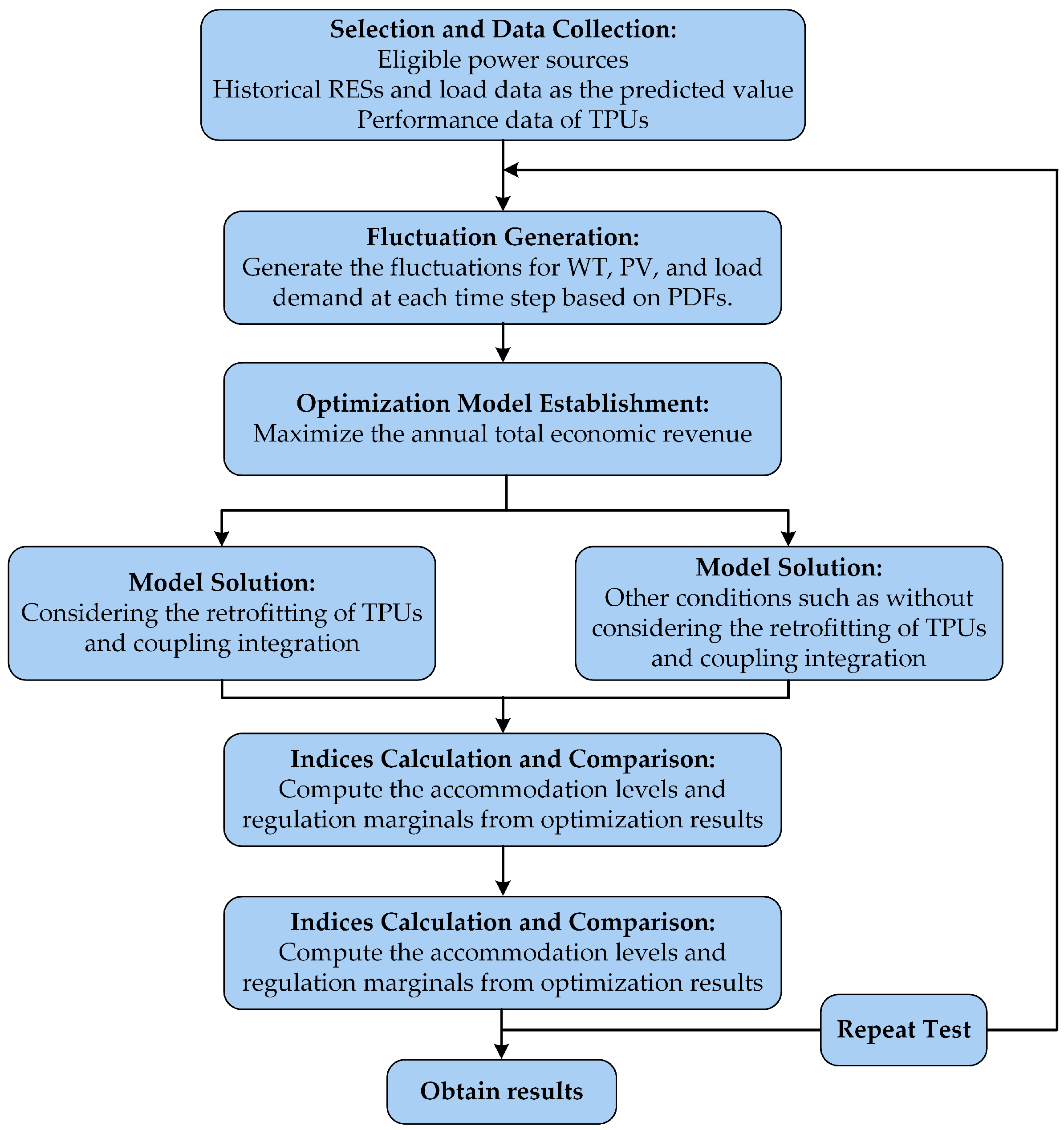
Figure 3.
Schematic diagram of the real-world project.

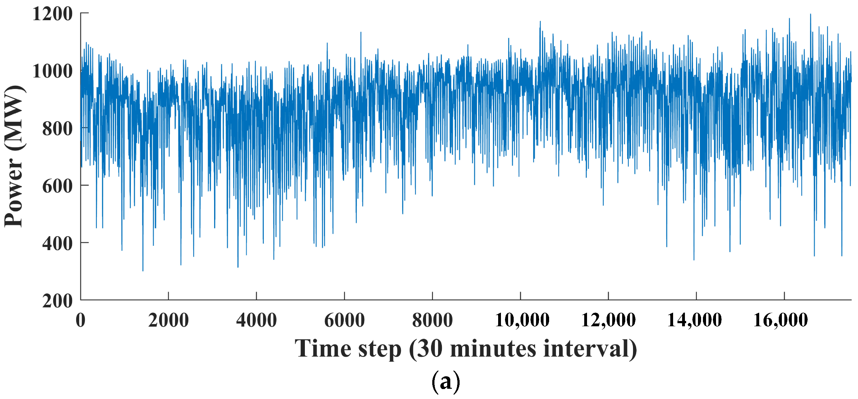
Figure 4.
Historical data of WT, PV, and load demand. (a) Wind data; (b) Photovoltaic data; (c) Load demand data.
Figure 4.
Historical data of WT, PV, and load demand. (a) Wind data; (b) Photovoltaic data; (c) Load demand data.
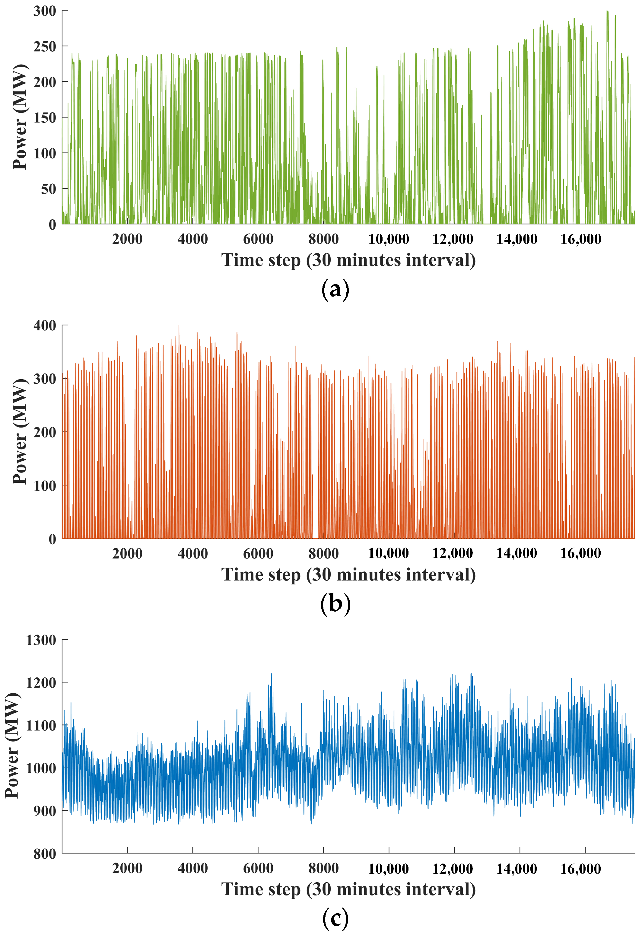
Figure 5.
Comparison of renewable energy curtailment. (a) After coupling integration with retrofitted TPUs; (b) Before coupling integration and without retrofitted TPUs.
Figure 5.
Comparison of renewable energy curtailment. (a) After coupling integration with retrofitted TPUs; (b) Before coupling integration and without retrofitted TPUs.
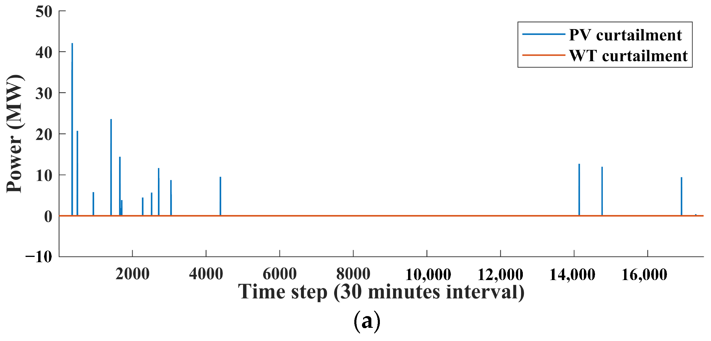
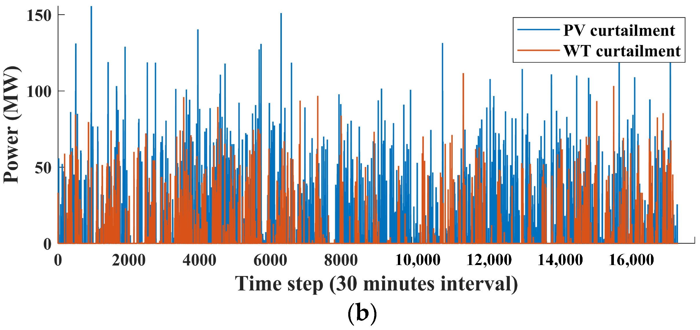
Figure 6.
Comparison of total output for thermal power units. (a) After coupling integration with retrofitted TPUs; (b) Before coupling integration and without retrofitted TPUs.
Figure 6.
Comparison of total output for thermal power units. (a) After coupling integration with retrofitted TPUs; (b) Before coupling integration and without retrofitted TPUs.


Table 1.
Comparison between CGS, BRTGS, and VPP.
| CGS | BRTGS | VPP | |
|---|---|---|---|
| Objective | Integration of geographically proximate large-scale RES and TPUs on the generation side | Transmission of large-scale RES and TPUs across the power grid | Management and coordination of distributed DERs or generation sources |
| Coordination Method | Utilization of local PCC | Deployment through the high-voltage transmission line | Primarily via the distribution network |
| Function | Mitigation of local RES fluctuations and provision of flexible support | Point-to-point stable power transmission | Integration of regulatory resources for flexible control |
Table 2.
Main performance parameters of the 600 MW TPU before and after retrofit.
| (MW/min) | (MW/min) | (MW) | (MW) | |
|---|---|---|---|---|
| Before | 9 | 6 | 300 | 180 |
| After | 18 | 12 | 300 | 150 |
Table 3.
Evaluation results before/after coupling integration and retrofitting of TPUs.
| After Coupling Integration with Retrofitted TPUs | Before Coupling Integration and without Retrofitted TPUs | Improvement | |
|---|---|---|---|
| (%) | 100 | 97.41 | 2.59 ↑ 1 |
| (%) | 99.97 | 95.28 | 4.69 ↑ |
| (%) | 99.99 | 96.39 | 3.6 ↑ |
| 154.0386 | 154.8457 | 0.08 ↓ | |
| 280.1582 | 212.1972 | 67.96 ↑ | |
| (MWh) | 6.1327 × 10⁵ | 5.9737 × 10⁵ | 1.59 × 10⁴ ↑ |
| (MWh) | 5.5930 × 10⁵ | 5.3302 × 10⁵ | 5.63 × 10⁴ ↑ |
| Annual revenues (CNY) | 2.1887 × 10⁹ | 2.1736 × 10⁹ | 1.51 × 10⁷ ↑ |
1 ↑: Improved value.
Table 4.
Evaluation results before/after considering retrofitting of TPUs in CGS.
| Coupling Integration with Retrofitted TPUs | Coupling Integration without Retrofitted TPUs [22] | Improvement | |
|---|---|---|---|
| (%) | 100 | 99.91 | 0.09 ↑ 1 |
| (%) | 99.97 | 97.84 | 2.13 ↑ |
| (%) | 99.99 | 98.92 | 1.07 ↑ |
| 154.0386 | 150.8950 | 3.14 ↑ | |
| 280.1582 | 207.8130 | 72.34 ↑ | |
| (MWh) | 6.1327 × 10⁵ | 6.1269 × 10⁵ | 0.058 × 10⁴ ↑ |
| (MWh) | 5.5930 × 10⁵ | 5.4737 × 10⁵ | 1.19 × 10⁴ ↑ |
| Annual revenues (CNY) | 2.1887 × 10⁹ | 2.1883 × 10⁹ | 0.038 × 10⁷ ↑ |
1 ↑: Improved value.
Disclaimer/Publisher’s Note: The statements, opinions and data contained in all publications are solely those of the individual author(s) and contributor(s) and not of MDPI and/or the editor(s). MDPI and/or the editor(s) disclaim responsibility for any injury to people or property resulting from any ideas, methods, instructions or products referred to in the content. |
© 2024 by the authors. Licensee MDPI, Basel, Switzerland. This article is an open access article distributed under the terms and conditions of the Creative Commons Attribution (CC BY) license (https://creativecommons.org/licenses/by/4.0/).
Share and Cite
MDPI and ACS Style
Zou, Y.; Xia, Q.; Chi, Y.; Wang, Q. Enhancing Renewable Energy Accommodation by Coupling Integration Optimization with Flexible Retrofitted Thermal Power Plant. Appl. Sci. 2024, 14, 2907. https://doi.org/10.3390/app14072907
AMA Style
Zou Y, Xia Q, Chi Y, Wang Q. Enhancing Renewable Energy Accommodation by Coupling Integration Optimization with Flexible Retrofitted Thermal Power Plant. Applied Sciences. 2024; 14(7):2907. https://doi.org/10.3390/app14072907
Chicago/Turabian StyleZou, Yao, Qinqin Xia, Yuan Chi, and Qianggang Wang. 2024. "Enhancing Renewable Energy Accommodation by Coupling Integration Optimization with Flexible Retrofitted Thermal Power Plant" Applied Sciences 14, no. 7: 2907. https://doi.org/10.3390/app14072907
Note that from the first issue of 2016, this journal uses article numbers instead of page numbers. See further details here.