PDED-ConvLSTM: Pyramid Dilated Deeper Encoder–Decoder Convolutional LSTM for Arctic Sea Ice Concentration Prediction

Abstract

Arctic sea ice concentration plays a key role in the global ecosystem. However, accurate prediction of Arctic sea ice concentration remains a challenging task due to its inherent nonlinearity and complex spatiotemporal correlations. To address these challenges, we propose an innovative encoder–decoder pyramid dilated convolutional long short-term memory network (DED-ConvLSTM). The model is constructed based on the convolutional long short-term memory network (ConvLSTM) and, for the first time, integrates the encoder–decoder architecture of ConvLSTM (ED-ConvLSTM) with a pyramidal dilated convolution strategy. This approach aims to efficiently capture the spatiotemporal properties of the sea ice concentration and to enhance the identification of its nonlinear relationships. By applying convolutional layers with different dilation rates, the PDED-ConvLSTM model can capture spatial features at multiple scales and increase the receptive field without losing resolution. Further, the integration of the pyramid convolution module significantly enhances the model’s ability to understand complex spatiotemporal relationships, resulting in notable improvements in prediction accuracy and generalization ability. The experimental results show that the sea ice concentration distribution predicted by the PDED-ConvLSTM model is in high agreement with ground-based observations, with the residuals between the predictions and observations maintained within a range from −20% to 20%. PDED-ConvLSTM outperforms other models in terms of prediction performance, reducing the RMSE by 3.6% compared to the traditional ConvLSTM model and also performing well over a five-month prediction period. These experiments demonstrate the potential of PDED-ConvLSTM in predicting Arctic sea ice concentrations, making it a viable tool to meet the requirements for accurate prediction and provide technical support for safe and efficient operations in the Arctic region.

1. Introduction

Global warming has become a widely acknowledged concern among the international community and the scientific world. Observational data indicate an accelerating trend in the melting of Arctic sea ice, influenced by the continuously rising atmospheric temperatures [1,2,3]. Against the backdrop of global warming, there has been a significant reduction in Arctic sea ice over the past few decades. This phenomenon, while impacting human activities and livelihoods, has also opened unprecedented opportunities for the exploitation of Arctic resources [4]. Particularly in the summer, the reduction in Arctic sea ice has created new commercial shipping routes, significantly shortening the journey between Asia and Europe [5,6]. Therefore, accurate and reliable ice forecasting is crucial for the interests of Arctic shipping and the planning of scientific exploration activities [7,8].

Sea ice concentration (SIC) denotes the percentage of a specific marine area covered by sea ice, reflecting the spatial density of sea ice and serving as one of the key parameters in characterizing sea ice. Methods for predicting sea ice concentration can be categorized into three types: numerical, statistical, and deep learning models. Numerical models integrate the thermodynamic and dynamic interactions between sea ice, seawater, and the atmosphere through physical equations [9,10], and they are commonly used for sea ice prediction [11,12]. Typical numerical models include the NCEP Climate Forecast System version 2 (CFSv2) developed by the NCEP Environmental Modeling Center, the U.S. Navy’s short-term sea ice forecast system (ACNFS), and the Arctic sea ice numerical forecasting system established by China’s National Marine Environmental Forecasting Center. Wang et al. conducted a thorough predictive analysis of the Arctic sea ice extent (SIE) from 1982 to 2007 using the Climate Forecast System version 2 (CFSv2) [13]. The Advanced Compact Naval Forecasting System (ACNFS) is capable of providing oceanic forecasts for the upcoming seven days [14,15], while the Arctic Sea Ice Numerical Forecasting System developed by China’s National Marine Environmental Forecasting Center can predict sea ice conditions up to five days ahead [16]. Sea ice forecasting products are crucial for shipping companies as they provide accurate and timely information about sea ice. This information helps them to plan shipping routes and avoid areas with sea ice, which reduces the risk of collision and improves navigation safety and efficiency [17]. Sea ice forecast products are also critical to the fishing industry, providing information on the extent, density, and structure of the sea ice cover. This information helps fishermen select the best areas to fish. Despite these advancements, numerical forecasting faces significant challenges in terms of computational requirements, predictive accuracy, and response time. Consequently, in predicting sea ice concentration, the performance of most numerical models often falls short of surpassing climatological average levels [18]. Statistical models are data-driven, establishing relationships between sea ice concentration and atmospheric conditions, oceanic conditions, and sea surface variables for prediction [19]. Vector autoregression (VAR) models [20] and linear Markov models are typical examples. Yuan et al. [21] used a linear Markov model trained with sea ice, ocean, and atmospheric variables from reanalysis data to predict Arctic sea ice concentrations on a monthly timescale. However, although statistical models offer a “lightweight” approach to predicting sea ice concentrations, they are unable to fully capture the nonlinear spatiotemporal relationships in long-term data sequences.

With the rapid advancement of artificial intelligence technology, deep learning has been successfully applied in fields such as oceanography, geography, and remote sensing. Due to its intelligent and lightweight characteristics, deep learning methods have been effectively utilized in addressing cryospheric challenges, such as sea ice detection [22], sea ice classification [23], and sea ice prediction. Compared to statistical and numerical models, deep learning models have shown improved accuracy in sea ice forecasting. In 2017, Chi and Kim [24] utilized long short-term memory (LSTM) networks to predict monthly Arctic sea ice concentrations. Their research indicated that this method outperformed autoregressive models in prediction accuracy and was comparable to the performance of the Sea Ice Prediction Network (SIPN). While LSTM networks are effective in capturing temporal features in data, they fall short in capturing spatial information. Kim et al. [25] developed a monthly sea ice concentration (SIC) prediction model using a convolutional neural network (CNN) model. The results indicated that the CNN model outperformed the baseline model, achieving a root mean square error (RMSE) of 0.06. The CNN model was effective in identifying and processing spatial information within the data, but it was less capable of capturing temporal information. Liu et al. [26] compared the performance of CNN and ConvLSTM models in predicting daily-scale Arctic SICs for the year 2018, using two days of data to forecast the following day’s sea ice concentration. The average RMSE for the CNN was 8.0%, while the ConvLSTM model showed an improvement, with an average RMSE reduced by 6.9%. The ConvLSTM model integrates the CNN and LSTM networks, capturing both temporal information and global spatial features through convolutional kernels. However, it still faces the temporal dependency issues inherent in recurrent networks, which could lead to the loss of historical information. Andersson et al. [27] introduced a U-net-based model, named IceNet, whose experimental results indicated that it surpassed common numerical and statistical models in binary accuracy (BACC) for sea ice extent estimation. While the downsampling operation effectively enlarges the receptive field, it may also lead to a loss in resolution, subsequently affecting the accuracy of pixel-level prediction tasks. He et al. [28] proposed a multi-layer stacking convolutional long short-term memory network (Multi-Stacking-ConvLSTM) for the daily-scale forecasting of Arctic SIC, with a prediction period of seven days. In this setup, the average RMSE for EOF+LSTM was 18.1%, for CNN+LSTM, it was 16.8%, and the Multi-Stacking-ConvLSTM improved sea ice concentration prediction accuracy to 5.3%. Ren et al. [29] proposed SICNet, a fully data-driven model for day-by-day sea ice prediction on subseasonal to seasonal scales. The experimental results demonstrate that the model achieves an average balanced accuracy (BACC) of over 90.0% during a 20-day prediction period, with an average BACC improvement of 1.8%. Huan et al. [30] developed the UNet-F/M model, based on the U-Net architecture, specifically for predicting Arctic sea ice melting and freezing periods. The UNet-F/M model demonstrated a significant reduction in mean absolute error (MAE) compared to the PredRNN++ model during a one-month prediction period, with a decrease of 2.0%.

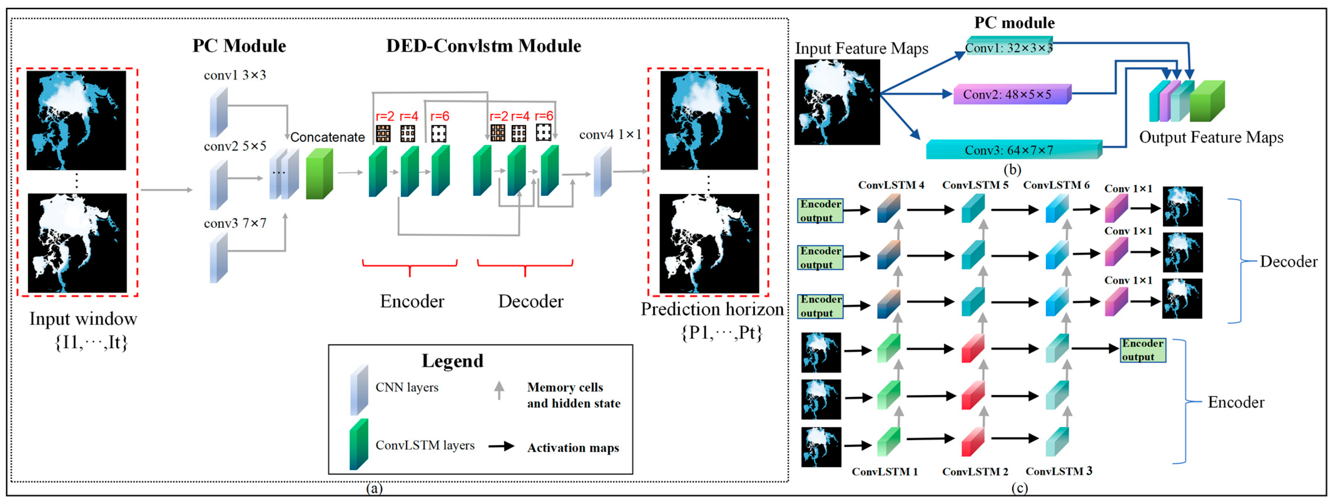
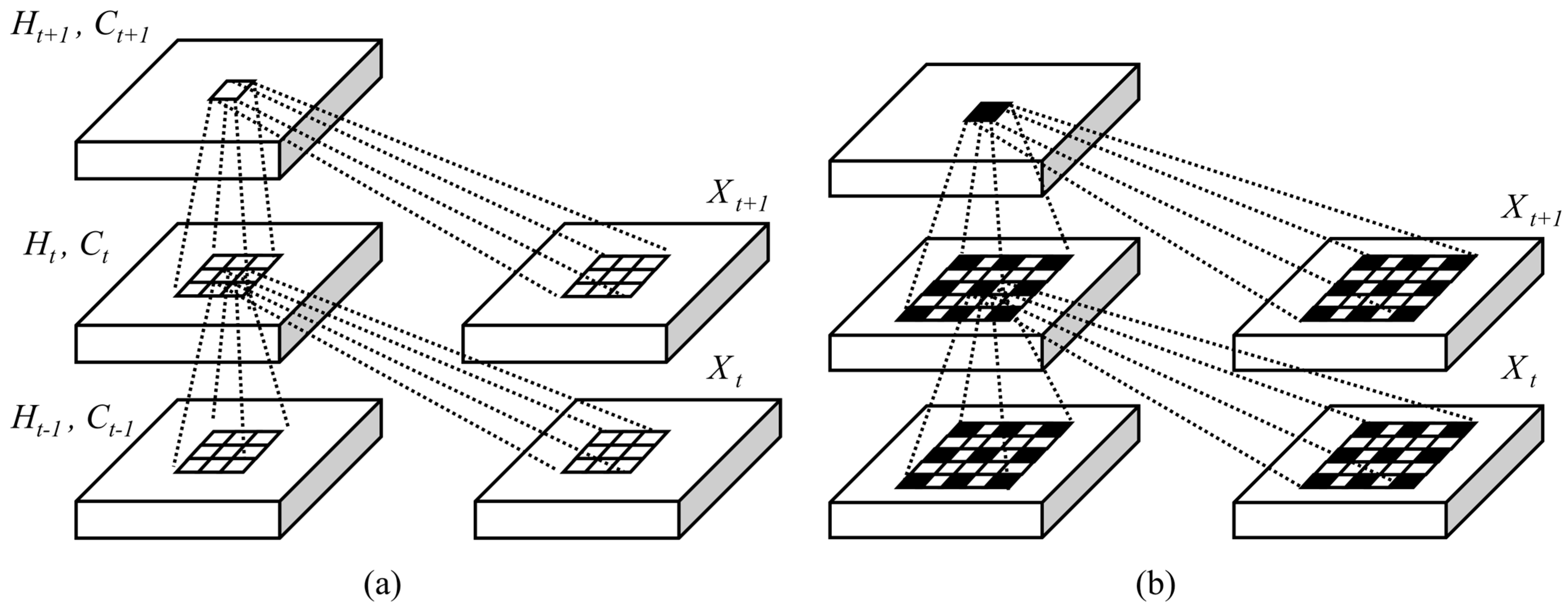
The forecasting of sea ice concentrations faces three main challenges. Firstly, traditional numerical and statistical models struggle to handle complex nonlinear relationships and lack computational efficiency. These models often have difficulty adapting to the diversity and complexity of Arctic sea ice concentration variations, resulting in a decreased prediction accuracy and generalization ability in practical applications. Secondly, traditional time-series methods often disregard early information when dealing with long time-series data. Since sea ice concentration forecasting heavily relies on long time-series data, neglecting historical information can directly impact the reliability and accuracy of model predictions. Additionally, as sea ice concentration prediction involves spatiotemporal series prediction, it is crucial to efficiently extract both temporal and spatial information. To address these challenges, we propose a deep recurrent neural network model based on the encoder–decoder architecture, named DED-ConvLSTM. This model learns temporal and spatial features through a cascading and more profound methodological approach. Building upon the ED-ConvLSTM framework, we have adjusted the dilation rates of each ConvLSTM layer to enlarge the receptive field. Additionally, to enhance the spatial learning capability of the DED-ConvLSTM model, we have integrated a Pyramid Convolution (PC) module, enabling multi-scale learning of spatial information. The specific contributions of our work are as follows:

(1)

We proposed a PDED-ConvLSTM model based on the ConvLSTM model. The model utilizes a PC module to learn spatial features at multiple scales, and a DED-ConvLSTM module is used to fuse the spatial information learned by the PC module with the spatial and temporal features learned by the ConvLSTM module. The PDED-ConvLSTM model can extract the global contextual spatiotemporal information from the sequence of Arctic sea ice concentrations more efficiently, and thus accurately perform Arctic sea ice concentration predictions.

(2)

In this study, we realized the prediction of Arctic sea ice concentrations over a long timescale and improved the accuracy of the prediction by fusing the Arctic sea ice concentration and the related influencing factors.

(3)

We explored the impact of typical oceanographic variables on forecasts of Arctic sea ice concentrations, with positive results for future research on sea ice prediction.

The rest of this paper is organized as follows: Section 2 demonstrates the proposed methodology of this study and Section 3 presents the experimental setup. The experimental results are analyzed and discussed in Section 4. Finally, this study is summarized in Section 5.

2. Proposed Methodology

As illustrated in Figure 1a, the PDED-ConvLSTM model consists of two key components: The first is known as the Pyramid Convolution (PC) module, designed for multi-scale extraction of spatially significant features. This is achieved through a set of convolutional layers with varying kernel sizes. The second module, termed Pyramid Dilated ED-ConvLSTM (DED-ConvLSTM), enhances the ED-ConvLSTM module by utilizing varied dilation rates of the convolutional kernels, enabling the learning of more profound spatial information. The DED-ConvLSTM module takes the spatial features learned from the PC module as input and outputs enhanced spatiotemporal saliency features, which are then utilized for the final prediction of the sea ice concentration sequence. Detailed information about each component will be provided in the following sections.

2.1. Capturing Spatiotemporal Features through the DED-ConvLSTM Module

The DED-ConvLSTM model implements two significant improvements to the standard ConvLSTM. First, it uses an encoder–decoder structure to efficiently process long-term sequence data. The encoder part encodes the hidden and cellular states of the entire input sequence and then passes them to the decoder. Its main work can be expressed as follows:

$${ h}_t^{enc}=f\left(W_{xh}^{enc}{x}_t+W_{hh}^{enc}{h}_{t-1}^{enc}+b_h^{enc}\right)$$

(1)

$$c_t^{enc}=g(W_{xc}^{enc}{x}_t+W_{hc}^{enc}{h}_{t-1}^{enc}+b_c^{enc})$$

(2)

where x_t is the input at the current time step of the input sequence, h_t and c_t are the hidden and cellular states at time step t, W and b are the network parameters, and f and g are the activation functions. The decoder uses these states as starting points to generate the output sequence, and the work of the decoder can be expressed as follows:

$$h_t^{dec}=f(W_{yh}^{dec}{y}_{t-1}+W_{hh}^{dec}{h}_{t-1}^{dec}+b_h^{dec})$$

(3)

$$y_t=softmax(W_{hy}^{dec}{h}_t^{dec}+b_y^{dec})$$

(4)

where y_t−1 is the output of the previous time step and y_t is the output of the current time step. This structure helps to maintain long-term time dependence and solve the time dependence problem in time-series forecasting. Second, DED-ConvLSTM introduces pyramidal dilated convolution based on ED-ConvLSTM. Dilated convolution is characterized by the application of its dilation rate. The dilation rate defines the spacing between elements within the convolution kernel, i.e., a certain number of intervals are inserted between each element of the convolution kernel to expand the input region it covers. Assuming that the dilation rate is denoted by r, the actual spacing of elements in the convolution kernel is r − 1 units. If the size of the standard convolutional kernel is k × k, then the actual size of the region covered by the convolutional kernel becomes k + (k − 1)(r − 1) in the dilated convolution. This structure allows the convolution kernel to achieve a wider sampling range of the input features without increasing the number of parameters. It effectively enhances the model’s ability to recognize spatial variability in sea ice concentration.

Before delving into the structure of DED-ConvLSTM, it is essential to first introduce the ConvLSTM model. Compared to the traditional LSTM network, the core concept of a ConvLSTM unit is to embody spatial correlations through shared weights, transforming the fully connected operations of the input, forget, and output gates in LSTM units into convolutional operations. This approach also takes into account the relationships between adjacent pixels and spatial context to model sequences [31].

The ConvLSTM model tends to “remember” only the short-term past of its sequence, as it cannot fully accumulate information about the entire sequence in its memory cells. However, in the task of sea ice sequence prediction, information from the long-term historical sea ice concentration is crucial for accurate forecasting. As shown in Figure 1c, the encoder considers information from all previous time points when processing the input sequence, while the decoder takes into account the overall contextual information provided by the encoder when generating predictions for each time point. Therefore, a ConvLSTM with an encoder–decoder structure should be employed to capture these long-term temporal dependencies.

To extract more comprehensively the spatiotemporal information, we have further expanded the ED-ConvLSTM model into a pyramid dilated convolutional structure. Specifically, this involves replacing the convolution operations in ED-ConvLSTM with pyramid dilated convolutions. Pyramid dilated convolutions offer significant advantages in the field of spatiotemporal prediction, particularly in enlarging the receptive field without information loss. Compared to traditional CNNs, they obviate the need for pooling to increase the receptive field, thereby avoiding the reduction in image size and the consequent loss of information. As shown in Figure 2, dilated convolutions allow for the observation of a broader range of information without reducing image resolution, addressing the issue of information loss during the process of downsizing and then upsizing in fully convolutional networks. Under the condition of maintaining a constant kernel size in the convolution process, the model is able to extract a greater amount of spatial information. This leads to the development of a more powerful ConvLSTM variant, termed the DED-ConvLSTM model.

2.2. Multi-Scale Capturing of Spatial Features through PC Modules

Typical CNN architectures are structured with a series of convolutional layers augmented by downsampling layers. While downsampling is beneficial for enlarging the receptive field, it compromises resolution, consequently affecting the precision of pixel-level predictions, a critical factor in tasks such as predicting sea ice concentration. Pyramid convolution [32] adeptly mitigates this limitation by altering the sizes of the convolutional kernels across different layers. The module employs different-sized convolutional kernels at different network layers, allowing the network to capture multi-scale features. At deeper network layers, pyramidal convolution can capture a wider range of spatial information using larger convolutional kernels, while at shallower network levels, it can retain higher spatial resolution and detailed features using smaller convolutional kernels. The advantage of this strategy is that it allows the network to extend its receptive field without sacrificing key spatial features, thus effectively balancing the size of the receptive field with the retention of spatial information. Pyramidal convolution provides a more comprehensive feature representation capability for the model through the integration of multi-scale features, especially when dealing with complex pixel-level tasks that require high spatial resolution.

As illustrated in Figure 1b, the PC module includes three convolutional layers with different kernel sizes. The sizes of the convolutional kernels in these layers are 3 × 3, 5 × 5, and 7 × 7, respectively. With the increase in kernel size, the number of channels in each layer also increase sequentially, with channel counts being 32, 48, and 64.

3. Experimental Settings

3.1. Datasets and Study Area

In this study, reanalysis data from the Arctic Ocean Physics Reanalysis product of the Copernicus Marine Service was used as the training set. The data originate from the Arctic Ocean and sea ice reanalysis based on the Coupled Ensemble Data Assimilation System (TOPAZ4b). TOPAZ4 relies on version 2.2 of the HYCOM ocean model and employs an Ensemble Kalman Filter data assimilation with 100 dynamic members. Beginning in 1991, a 30-year reanalysis of the Arctic Ocean and sea ice was conducted and is provided as a multi-year physical product by the Arctic Ocean Forecasting Center (ARC MFC), which is part of the Copernicus Marine Environment Monitoring Service.

The spatial resolution of the data is 12.5 × 12.5 km, and the study focuses on the Arctic core area defined by a grid of 528 × 512 cells (90 N, 50 N, 180 E, and 180 W), spanning 20 years from 2000 to 2020. The study area is depicted in Figure 3. Predicting sea ice concentration in the Arctic during the melt season is of significant importance for national entities and relevant enterprises in assessing future shipping potential. It also aids scientists in gaining a more comprehensive understanding and quantification of the pace and extent of climate change. Therefore, our focus will be on predicting the melting period from May to September each year. This period is when Arctic sea ice melting is most active, and studying the changes in sea ice concentration during this time will provide us with critical information and insights.

Table 1. Information on sea ice concentrations and influencing factors.

Feature	Source	Units
Sea Ice Concentration	Copernicus Marine Service	Dimensionless
Sea surface temperature	Copernicus Marine Service	°C
Sea surface salinity	Copernicus Marine Service	PSU
Sea ice thickness	Copernicus Marine Service	M

provides a detailed description of the specific parameters used as model inputs from the Copernicus Marine Service dataset, namely, sea water salinity, sea surface temperature, and sea ice thickness.

In the data preprocessing stage, we set the anomalous sea ice data (grid point data with sea ice concentration less than 0 or greater than 1) to 0. Then, the Arctic sea ice concentration and other ocean factor data were initialized to fit the input dimensions (number of samples, time steps, widths, heights, and number of channels) of the PDED-ConvLSTM model. Finally, sea ice concentration and other ocean factor features were fused into the channel dimension. The model uses the rolling window method to input the training data Ii-2 to Ii, and generates the predicted values of Arctic sea ice concentration Pi + 1 to Pi + 2 in the prediction layer.

3.2. Parameters and Metrics

The experiments conducted in this study were carried out using TensorFlow 2.6.0. The Adam optimizer was employed, with a batch size set to 4 and a learning rate of 0.001. The training process was conducted over 100 epochs. To prevent overfitting of the model, techniques such as dropout and early stopping were utilized.

To validate our predictions, we employed root mean square error (RMSE), mean absolute error (MAE), Pearson correlation coefficient (PCC), and Nash–Sutcliffe efficiency (NSE) as evaluation metrics. RMSE and MAE are common metrics in regression tasks used to measure the absolute differences between predicted and actual values, with smaller values indicating better predictive ability. NSE and PCC are used to describe the correlation between predicted and actual values, with values closer to 1 indicating better correlation of model predictions. The definitions are as follows:

$$\mathrm{RMSE}=\sqrt{\frac{1}{n}\sum _{i=1}^N{\left(\frac{Tru{e}_i-Predic{t}_i}{Tru{e}_i}\right)}^2}$$

(5)

$$\mathrm{MAE}=\frac{1}{N}{{\displaystyle \sum }}_{i=1}^N\mid Tru{e}_i-Predic{t}_i\mid$$

(6)

$$\mathrm{PCC}=\frac{{\displaystyle \sum _{i=1}^N}\left(Tru{e}_i-\overline{True}\right)\left(Predic{t}_i-\overline{Predict}\right)}{\sqrt{{\displaystyle \sum _{i=1}^N}{\left(Tru{e}_i-\overline{True}\right)}^2{\displaystyle \sum _{t=1}^N}{\left(Predic{t}_i-\overline{Predict}\right)}^2}}$$

(7)

$$\mathrm{NSE}=1-\frac{{\sum }_{i=1}^N{\left(Tru{e}_i-Pedic{t}_i\right)}^2}{{\sum }_{i=1}^N{\left(Tru{e}_i-\overline{Pedic{t}_i}\right)}^2}$$

(8)

where the observed data are represented by True and the predicted values are represented by Predict.

4. Experiment and Results

4.1. Ablation Study

Ablation experiments were performed on the PDED-ConvLSTM model to evaluate the effectiveness of the key components. Three variants of the PDED-ConvLSTM model were designed as follows:

(1)

NO_PC: in this variant, the PC module for multi-scale extraction of spatial information is removed from PDED-ConvLSTM.

(2)

NO_ED: in this variant, the encoder–decoder structure for processing long sequences is removed.

(3)

NO_PD: this is a variant without the pyramidal dilated convolution, which is designed to increase the sensory field without increasing the number of parameters.

Table 2. Ablation experiment.

Model	Encoder Decoder Structure	Pyramid Dilated Convolution	PC Module	RMSE	MAE	PCC	NSE
NO_PC	✔	✔		0.089	0.035	0.958	0.927
NO_ED		✔	✔	0.087	0.035	0.961	0.928
NO_PD	✔		✔	0.092	0.041	0.942	0.911
PDED- ConvLSTM	✔	✔	✔	0.073	0.022	0.971	0.940

✔ implies that the model has a corresponding function.

lists the performance differences between the three variants and PDED-ConvLSTM. Compared with NO_PC, the PDED-ConvLSTM model has smaller prediction errors and higher correlation coefficients. The results show that multi-scale extraction of spatial features using the PC module is effective in improving the prediction results. The substantial decrease in the predictive ability of NO_PD suggests that the pyramidal dilated convolution in PDED-ConvLSTM can improve the prediction ability substantially. Arctic sea ice concentration prediction is a long time-series prediction task, and NO_ED lacking the encoder–decoder structure reduces the ability to handle long time sea ice series. Therefore, the encoder–decoder structure is necessary.

4.2. Overall Performance of PDED-ConvLSTM

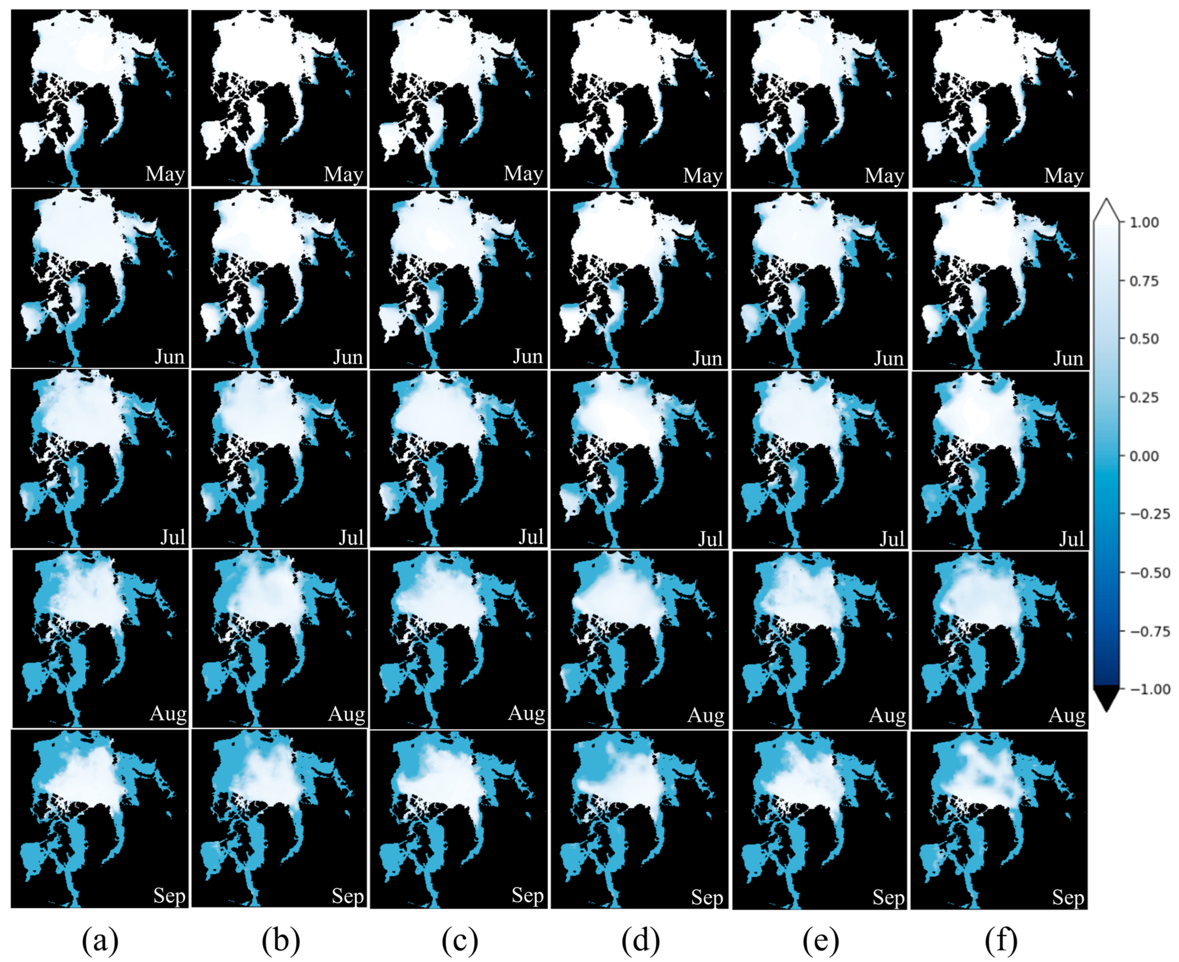
The spatial distribution of the predicted values and ground-truth during the melt season (May to September) from 2018 to 2020 is shown in Figure 4. The PDED-ConvLSTM model proposed in this paper accurately captures the sea ice melting process. The spatial distribution of the predicted sea ice concentration closely resembles the ground truth, with a clear delineation of the ice edges. The PDED-ConvLSTM model particularly excels from May to July when the sea ice concentration (SIC) is higher, while its performance slightly decreases in August and September when the SIC is lower. Specifically, the model tends to underestimate sea ice concentration (SIC) on the Pacific side of the Arctic Ocean, especially in the Beaufort Sea, Chukchi Sea, and East Siberian Sea. Overall, the PDED-ConvLSTM model proposed in our study demonstrates commendable performance both in months with stable SIC variations and those with high variability.

We explored the advantages of the PDED-ConvLSTM model over other deep learning models based on evaluation metrics. The selected models for comparison include ConvLSTM, Climatology, and Multi-Stacking ConvLSTM. The Climatology model represents the average SIC at the same time each year over the preceding 10 years of the respective target prediction time. It is a forecasting method based on the average of historical data, commonly used in climate change and meteorological studies as a baseline model.

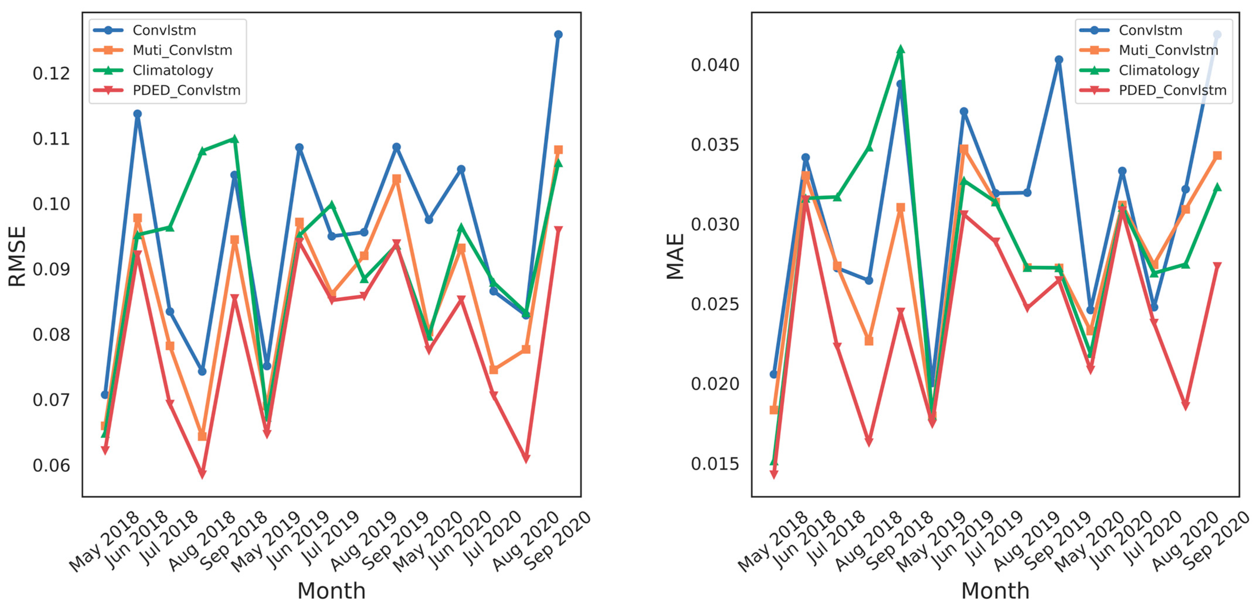
As depicted in Figure 5, the trends in RMSE and MAE predicted by our proposed method in comparison to other methods are presented. The results demonstrate that the three deep learning models exhibit similar trends in RMSE/MAE. The PDED-ConvLSTM model shows lower RMSE/MAE values than the other models, indicating its superior precision. The performance of the Climatology model is comparable to that of the Multi-Stacking ConvLSTM, with the ConvLSTM model showing the least favorable results. The Climatology model, which predicts concentrations based on average values, exhibits a different trend compared to the deep learning models. Compared to Climatology, ConvLSTM, and Muti-Stacking ConvLSTM, the PDED-ConvLSTM model reduces the average RMSE and MAE from 2018 to 2020 by 3.5%, 3.6%, and 2.1%, and by 2.7%, 2.9%, and 1.8%, respectively. The results show significant advantages of the PDED-ConvLSTM model over existing models. The ConvLSTM model can capture both temporal and spatial information. The Muti-Stacking ConvLSTM model, although improving the performance of the model through multiple stacked network layers, still struggles with long time series. The Climatology model bases its predictions on historical averages, limiting its ability to deal with dynamic trends with a certain degree of flexibility and accuracy.

The results presented in

Table 3. NSE And PCC predicted by different models.

Metrics	Model	2018	2019	2020
NSE	Climatology	0.946	0.940	0.933
	ConvLSTM	0.930	0.919	0.919
	Muti Stacking-	0.943	0.931	0.931
	ConvLSTM
	PDED-	0.948	0.934	0.939
	ConvLSTM
PCC	Climatology	0.973	0.970	0.967
	ConvLSTM	0.966	0.961	0.960
	Muti Stacking-	0.971	0.964	0.965
	ConvLSTM
	PDED-	0.975	0.968	0.971
	Con vLSTM

indicate that our proposed PDED-ConvLSTM model demonstrates superior performance, achieving the lowest PCC and NSE values compared to other deep learning models. The average NSE and PCC values of the PDED-ConvLSTM model are 0.941 and 0.971, respectively. The improvement as a result of this model over ConvLSTM and Muti-Stacking ConvLSTM in NSE is 1.9% and 0.5%, and in PCC, it is is 1% and 0.9%, respectively. The Climatology model and the PDED-ConvLSTM model exhibit similar correlation performance. This phenomenon occurs because the Climatology model’s predictions are based on the historical output data’s average. The results show that the predictions of the PDED-ConvLSTM model are more highly correlated with the ground-truth values and are able to capture the trends in the sea ice concentration series.

To evaluate the efficiency of the proposed method, we assess the time complexity of PDED-ConvLSTM based on FLOPs (floating-point operations), which is defined as the number of floating point operations per second and is commonly used as a measure of the time complexity of deep learning models. The results of the FLOP comparison between PDED-ConvLSTM and other deep learning models are shown in

Table 4. The results of the three models on the FLOP indicator.

Model	FLOPs
ConvLSTM	21.6
Muti-Stacking ConvLSTM	53.8
PDED-ConvLSTM	44.6

. Compared with the ConvLSTM model, although the FLOPs of PDED-ConvLSTM are higher than those of ConvLSTM, its performance is significantly better than the latter. Compared to Multi-Stacking ConvLSTM, PDED-ConvLSTM achieves higher prediction accuracy with lower time complexity, demonstrating its optimization in computational resource utilization.

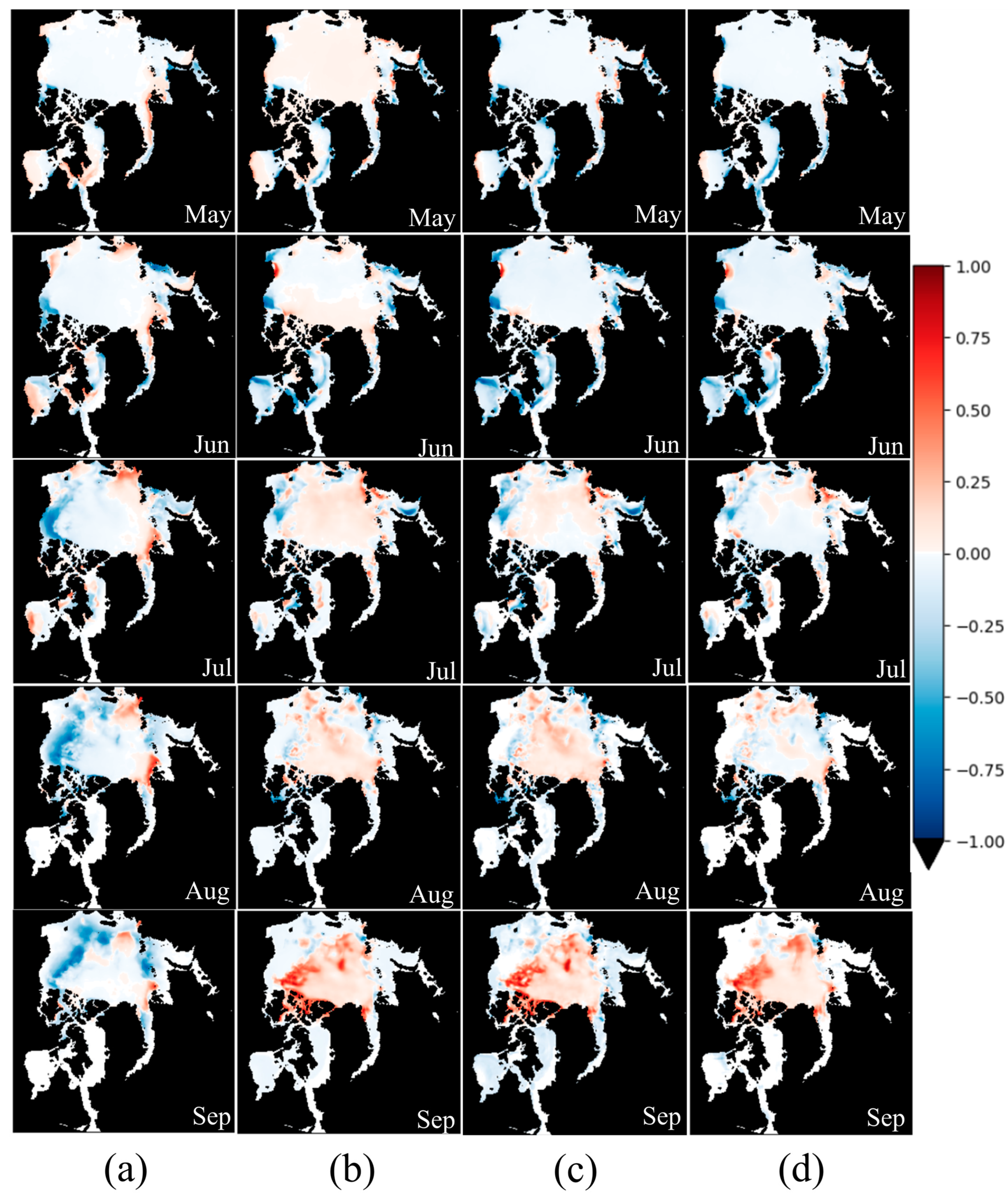
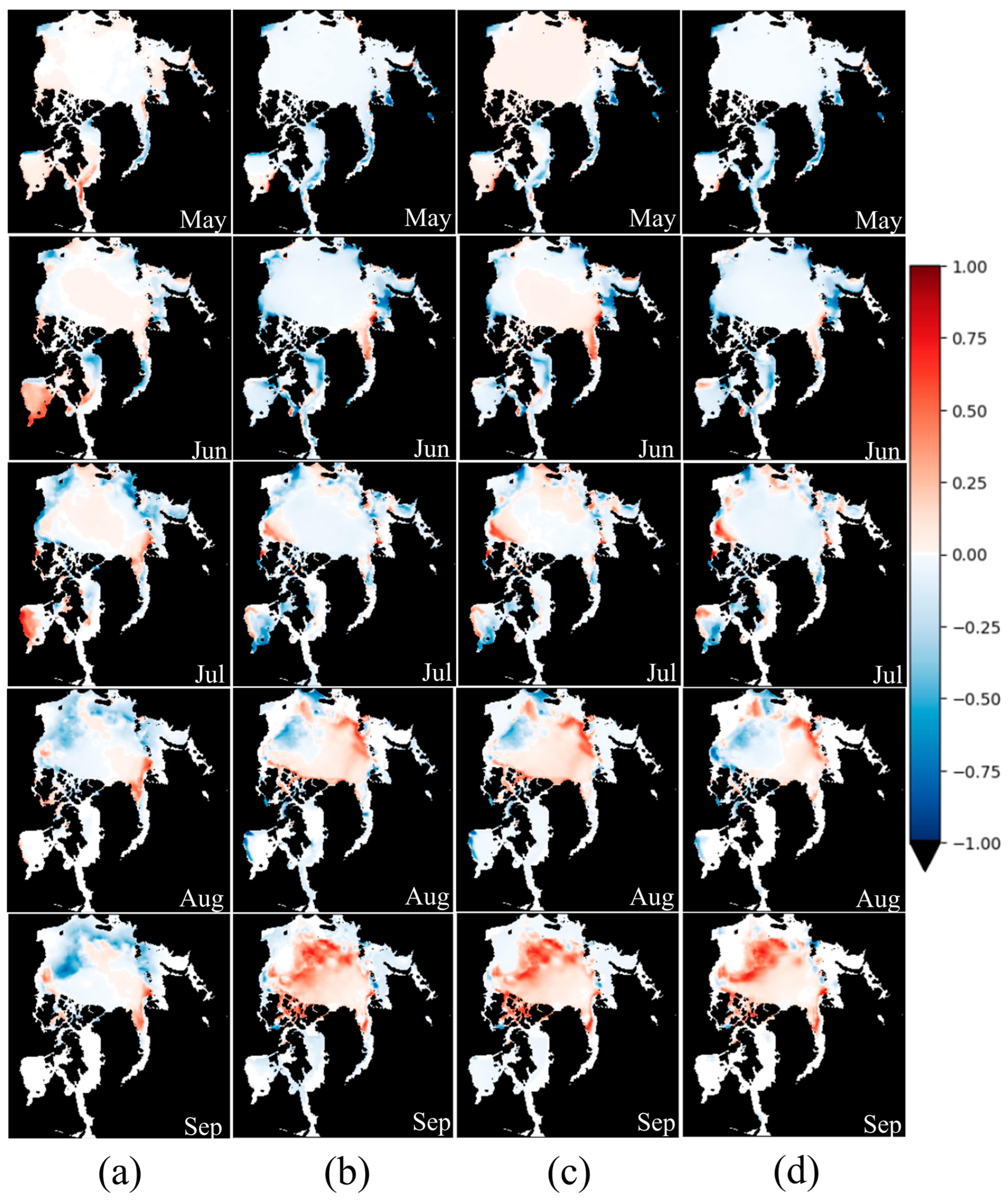
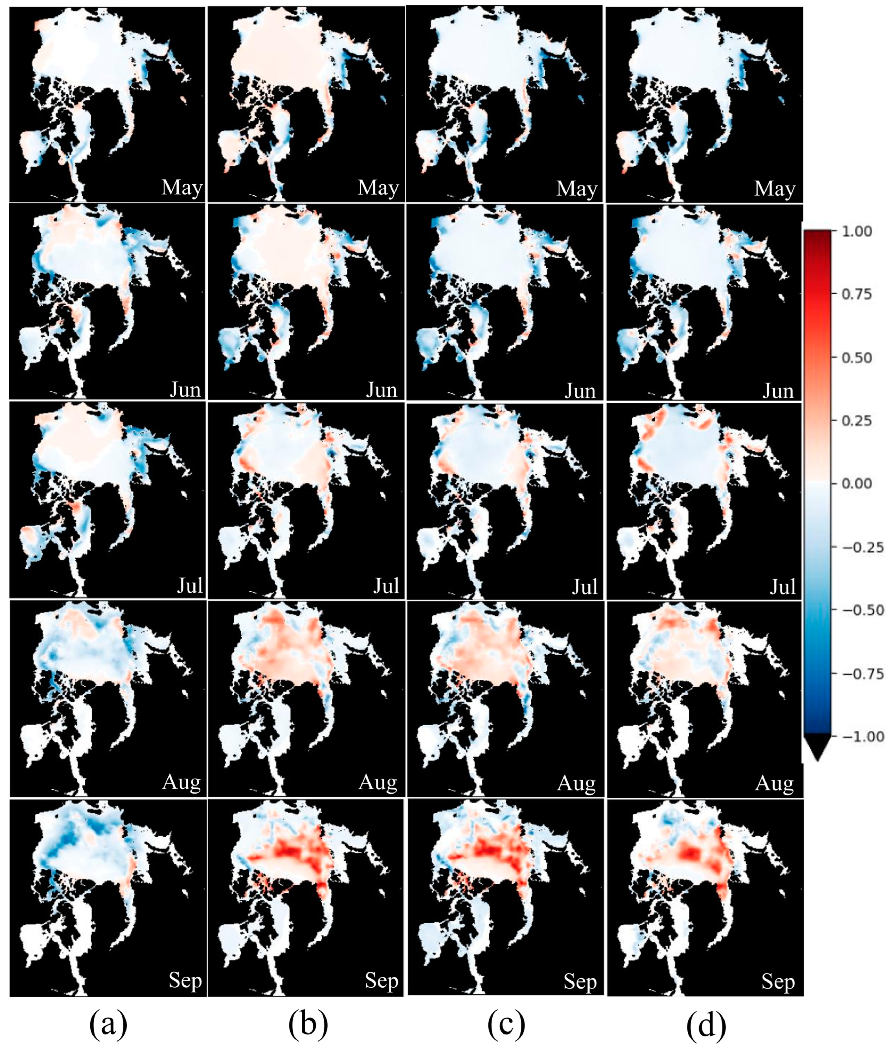
In this study, we further evaluated the performance of our proposed model by analyzing the differences between the predicted values and ground-truth observations from 2018 to 2020 (Predict–Ground Truth). As illustrated in Figure 6, Figure 7 and Figure 8, red areas indicate an overestimation of sea ice concentration (Predict − True > 0), while blue areas indicate an underestimation (Predict − True < 0), with deeper colors signifying larger discrepancies. The results reveal that the errors in predictions are primarily concentrated in the areas of first-year ice, with smaller errors in multi-year ice zones. The Climatology model tends to underestimate sea ice concentrations in most cases, whereas deep learning models generally overestimate it. Our proposed PDED-ConvLSTM model demonstrates superior performance in the majority of the study area, with lighter shades and smaller areas of both overestimation and underestimation, indicating the highest accuracy in predictions.

The errors were primarily found in the Kara Sea and Barents Sea, likely due to the intensified amplitude of the El Niño-Southern Oscillation (ENSO) during the climate-warming process, which causes significant interannual variability in the SIC of these seas during winter [33]. This leads to larger prediction errors in these marine areas. Additionally, the drift of sea ice through the Beaufort Sea also results in noticeable SIC variations, subsequently increasing the prediction errors in this region [34].

4.3. Performance with a Five-Month Lead Time

Current Arctic sea ice prediction models primarily operate on subseasonal to seasonal timescales, with a lead time of approximately three months for forecasts. Achieving predictions over longer timescales remains a significant challenge. To test the performance of our model proposed for long-term timescale predictions, we set the lead time to five months.

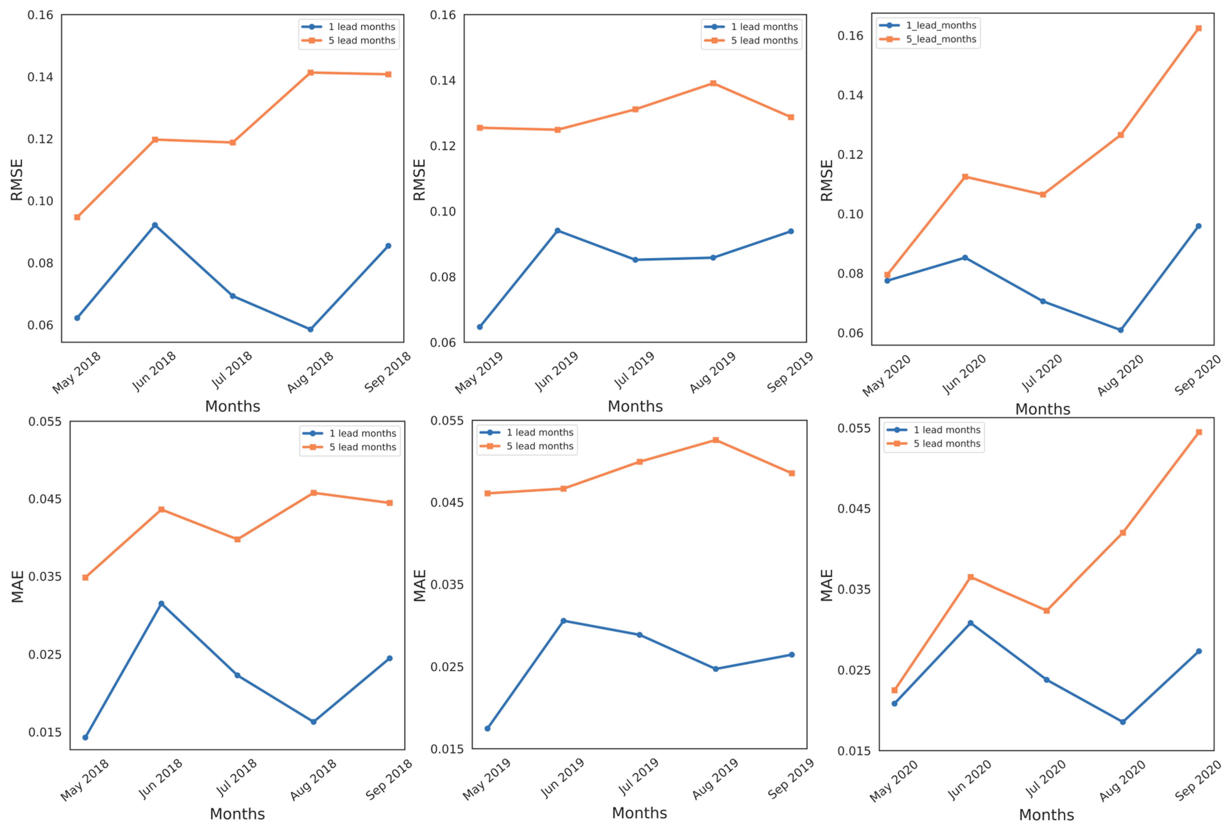
Figure 9 displays the trends of RMSE and MAE for different lead times from 2018 to 2020. The RMSE and MAE values for a five-month lead time are lower than those for a one-month lead time. The average RMSE value for a five-month lead time is 0.121, showing a reduction of 0.044 compared to the one-month lead time average RMSE. As can be seen from the PCC and NSE results in

Table 5. NSE And PCC predicted by different lead months.

Metrics	Length of Input SIC Sequence	2018	2019	2020
NSE	1-Month Lead	0.948	0.934	0.939
	5-Month Lead	0.929	0.917	0.914
PCC	1-Month Lead	0.975	0.968	0.971
	5-Month Lead	0.961	0.944	0.958

, setting a lead time of five months decreases the correlation between the predicted results and the actual values. This decrease is attributed to the lengthening of the prediction sequence, which weakens the model’s performance. Nonetheless, the performance of our proposed model with a five-month lead time is still comparable to that of the one-month ConvLSTM model. This is because the encoder in the PDED-ConvLSTM model considers all historical sea ice concentration information when processing the input sequence, thereby avoiding the phenomenon of information loss.

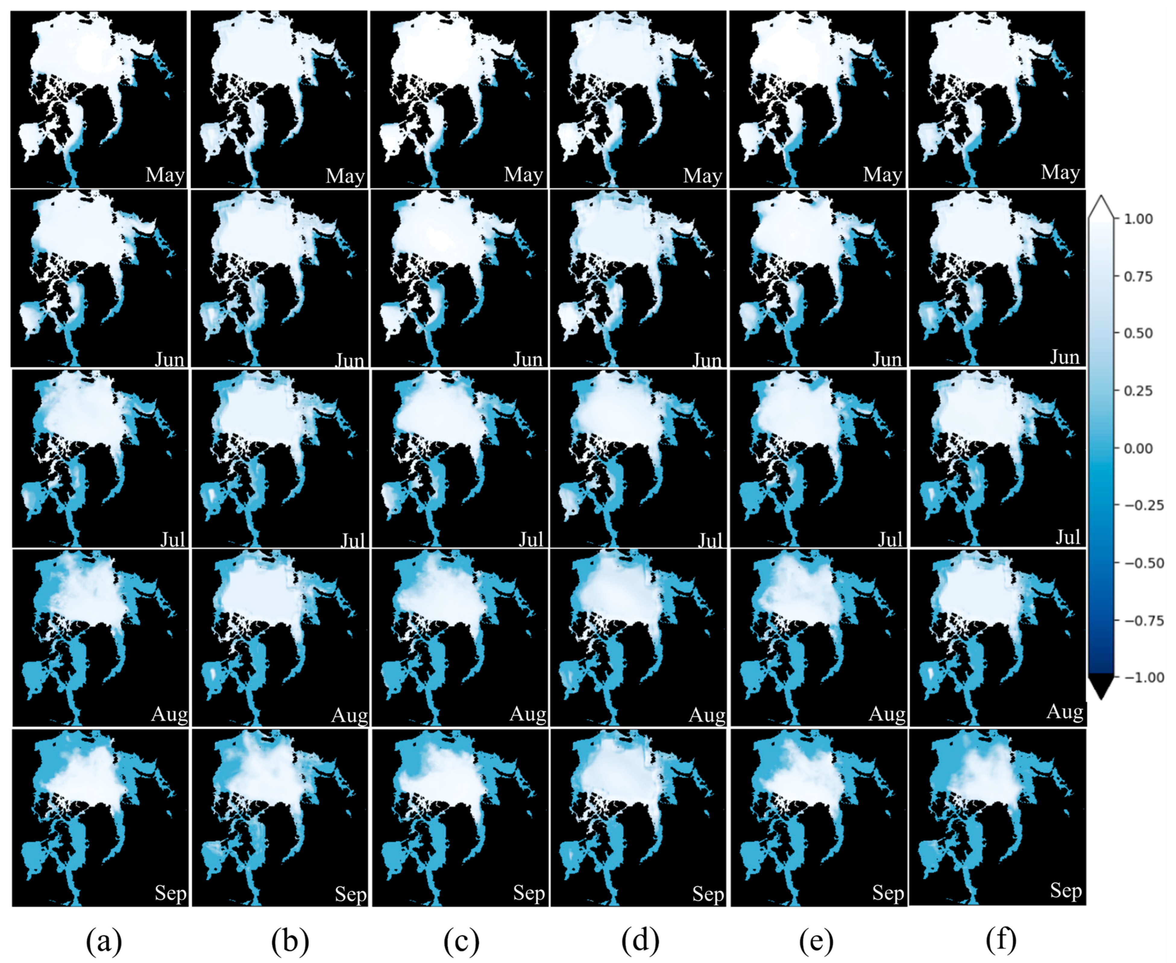
Figure 10 illustrates the spatial distribution of the predicted values and the ground truth for the melt seasons of 2018–2020, with a lead time of five months. Although the accuracy of these predictions, in terms of their alignment with the ground-truth data, is reduced compared to the one-month lead time forecasts, the predictions still accurately capture the dynamic changes in sea ice. Therefore, these forecasts continue to provide reliable information for shipping navigation and Arctic scientific research.

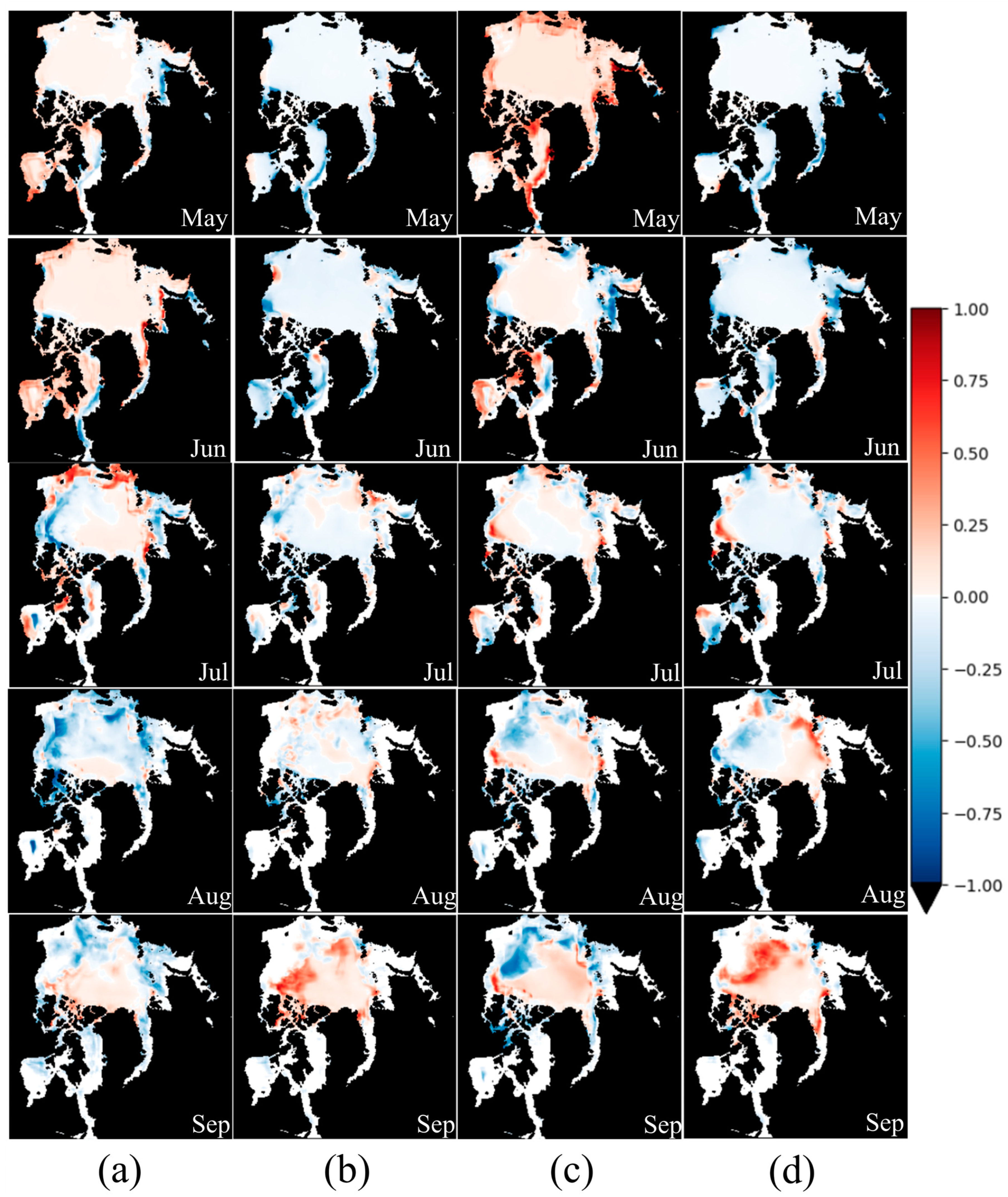
Figure 11 represents the spatial distribution of residuals for the melt seasons from 2018 to 2019. It is evident that the errors are larger with a five-month lead time compared to a one-month lead time. In the first two months of the five-month lead time, most errors fall within the range of (−10%, 10%). In the subsequent three months, the errors gradually increase but are mostly kept within the range of (−25%, 25%). Additionally, compared to the one-month lead time, the five-month lead time consistently underestimates the one-year ice area in the Arctic, while the one-month lead time consistently overestimates it.

From the prediction results over these two years, it can be concluded that for the prediction of Arctic sea ice during the melt season, the PDED-ConvLSTM model is capable of keeping the error range for most regions within (−20%, 20%), which is considered an ideal outcome.

4.4. Exploring the Effects of Different Impact Factors on Arctic Sea Ice Prediction

We investigated how typical oceanic influencing factors affect the prediction of Arctic sea ice, which aids in enhancing the selection of model input variables, thereby improving the model’s accuracy and effectiveness. We selected three typical oceanic factors: sea surface temperature (SST), sea water salinity (SALT), and sea ice thickness (THIC). The method of integrating oceanic influencing factors involves overlaying SIC with SST, SALT, and THIC, respectively, and then inputting these data into the PC module. The output feature map is then fed into the main network to obtain the final prediction results. We evaluated the impact of specific parameters using RMSE (root mean square error) and MAE (mean absolute error), with a lower RMSE value indicating a greater influence of that parameter on the PDED-ConvLSTM model’s predictions.

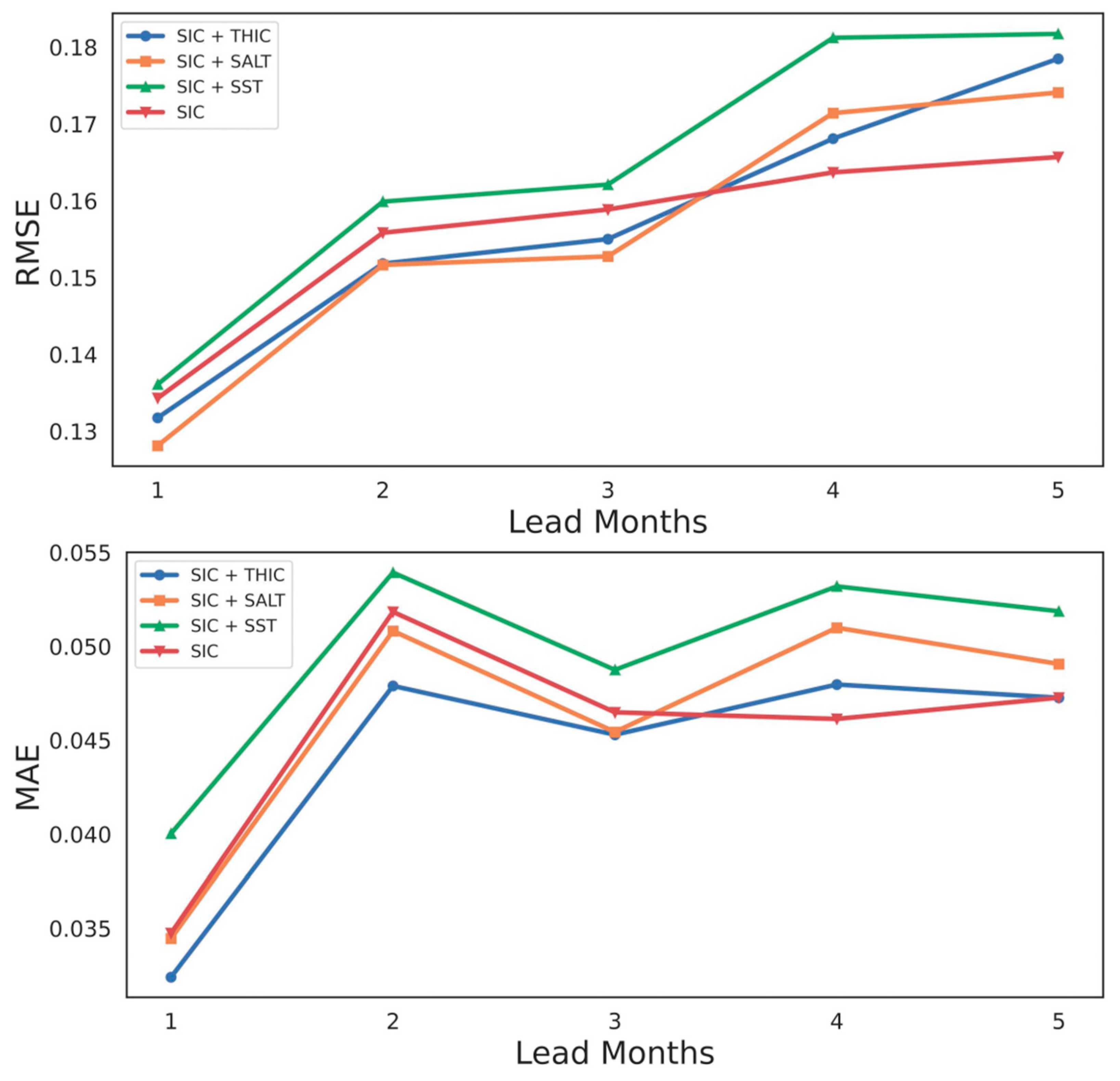
Figure 12 displays the RMSE trends for different input parameters in the PDED-ConvLSTM model during the 2018 melt season. SST consistently shows a noticeable negative contribution throughout all times, while SALT and THIC have both positive and negative impacts. During the May to July, the inclusion of SALT and THIC positively contributes to the forecast, resulting in lower RMSE/MAE values. However, in August and September, all influencing factors contribute negatively to the prediction.

In summary, during the melting season, SST has a negative impact on SIC predictions with a five-month lead time. SALT and THIC positively contribute to predictions before August and negatively after August. Therefore, if we are predicting SIC from May to July, THIC and SALT should be added as inputs. If the prediction is from August to September, only SIC should be used as an input.

5. Conclusions

In this paper, we proposed the PDED-ConvLSTM model, based on ConvLSTM, for the monthly-scale prediction of Arctic sea ice. The PDED-ConvLSTM model comprised the Pyramid Convolution (PC) module and the DED-ConvLSTM module. The DED-ConvLSTM module utilized spatial features learned from the PC module as the input and outputted enhanced spatiotemporal saliency features for the final prediction of the sea ice concentration sequence. This study’s findings revealed that the PC module effectively performed multi-scale spatial feature extraction, particularly for SIC data, by expanding its receptive field. In addition, more in-depth and detailed information mining was realized in the DED-ConvLSTM module for long-term historical SIC data, which improved the predictive capability of the model. To assess the model’s performance, this study utilized the following performance metrics: RMSE, MAE, PCC, and NSE. The results indicated that the PDED-ConvLSTM model outperformed the other two deep learning models and the traditional climatological model in terms of prediction accuracy. The PDED-ConvLSTM model showed a reduction of 3.6% and 2.9% in the average RMSE and MAE values, respectively, compared to the ConvLSTM model from 2018 to 2020. This suggested a significant improvement in reducing prediction errors. The numerical improvements showcased the efficiency and reliability of the PDED-ConvLSTM model and its potential application in predicting sea ice concentrations.

This study further explored the predictive performance of the model under a five-month lead-time condition. It was found that as the lead time was extended, the difficulty for the model to learn the complex nonlinear relationship between SIC and time correspondingly increased. Specifically, when the lead time was extended from one month to five months, the average RMSE value of the model only decreased by 0.04. This phenomenon was attributed to the model’s encoder part, where the processing of the input sequence took into consideration the SIC information from all historical time points. Meanwhile, the decoder effectively utilized the global SIC information provided by the encoder when generating predictions for each respective time point. Consequently, the PDED-ConvLSTM model demonstrated significant advantages in long-term timescale prediction.

In the final part of our study, we meticulously examined the impact of three environmental factors, sea water salinity, sea ice thickness, and sea surface temperature on the prediction of SICs. It was particularly noteworthy that sea surface temperature exhibited a significant negative impact on SIC prediction during the melt season. Conversely, sea water salinity and sea ice thickness contributed positively to predictions during the relatively stable period from May to July for SICs. However, these factors shifted to have a negative impact during the months between August and September, when SICs underwent more dramatic changes. This discovery shed light on the complex interplay of different environmental factors in sea ice prediction, especially across varying seasons and stages of sea ice variation. This research study has provided a crucial theoretical foundation for the integration of environmental factors in sea ice concentration prediction models and laid the groundwork for future in-depth studies in this field.

The following outlines some prospects for future work. While this study has already encompassed the relationship between sea ice concentration (SIC) and three oceanic factors, future efforts should focus on expanding the variety of oceanic influencing factors and increasing the volume of sample data. This would facilitate a more in-depth understanding of the complex interactions between sea ice concentration and other potential predictive factors. Moreover, determining the optimal lengths for input and output sequences is crucial for enhancing the accuracy and reliability of sea ice concentration predictions. Through these approaches, we can anticipate significant advancements in the precision and efficiency of sea ice concentration forecasts, thereby providing a more robust scientific foundation for future climate modeling and environmental policy making.