
Energy Efficiency Improvement in Reconfigurable Photovoltaic Systems: An Evaluation of Team Systems


Eastern Barcelona School of Engineering (EEBE), Technical University of Catalonia-BarcelonaTech (UPC), Eduard Maristany Ave. 16, E-08019 Barcelona, Spain
*
Author to whom correspondence should be addressed.
Appl. Sci. 2024, 14(8), 3368; https://doi.org/10.3390/app14083368
Submission received: 15 March 2024
/
Revised: 4 April 2024
/
Accepted: 13 April 2024
/
Published: 16 April 2024
(This article belongs to the Collection Improvements in the Production, Monitoring, Management and Impact on the Grid of Photovoltaic Installations)
Abstract
:The main objective of this work is to evaluate the energy efficiency improvement obtained in grid-connected photovoltaic systems based on a dynamic reconfiguration strategy. The MIX and team reconfigurable photovoltaic system topologies have been considered since both minimize the operation of the inverters in low-load conditions. A numerical method is used to analyze the energy flows within the photovoltaic system, with a specific focus on the plant-oriented configuration. In this work, MIX systems are only presented briefly, while team reconfigurable photovoltaic systems are analyzed in more detail. This is because team systems can be implemented using conventional commercial inverters, electromechanical switches to redirect power flows, and a simple digital controller (as based on the Arduino platforms). The energy supplied to the grid by two grid-connected photovoltaic systems will be evaluated: one based on a classic non-reconfigurable strategy and another based on the team strategy. The measurement of the energy generated by these two systems, tested under various irradiance levels (emulating different climatic conditions), shows that reconfigurable systems always exhibit greater energy efficiency. However, this energy improvement can only be considered substantial in certain situations.
1. Introduction
As stated by the Energy Department of the European Commission, energy is the commodity that fuels the economy, and the prosperity and security of the EU depend on a stable and affordable energy supply [1]. The changes driven by the EU’s energy policies have led to a significant reduction in the use of the most polluting fuels, with consumption shifting towards natural gas and renewables.
The decrease in gas production in the EU in recent years (a 2.5% drop over the last 10 years [2]) has resulted in a greater dependence on gas imports. To reduce this dependence on foreign resources, it is necessary to increase energy production using domestic resources. In this regard, the intensive use of renewable energies and high-efficiency systems will play a crucial role.
Regarding renewables, photovoltaic (PV) solar energy has shown the highest growth in Europe in the last 10 years, reaching 186 GW installed by the end of 2021, an increase of close to 150% [3]. While this is a step in the right direction, it is important to also consider increasing the efficiency of PV systems.
Inverters used in grid-connected PV (GCPV) systems are highly efficient (typically 92–98% in commercially available inverters [4,5]), with some room for improvement, but the industry is currently focused on increasing the efficiency of solar panels. According to data published by the National Renewable Energy Laboratory (NREL), the currently highest confirmed conversion efficiency for PV modules ranges between 14% and 25% [6], depending on the PV technology considered, values that coincide with those previously collected in the [7]. Another approach worth exploring is the improvement of energy efficiency through the use of reconfigurable PV systems in grid-connected applications.
The plant-oriented (PO) configuration is the most prevalent architecture used in large-scale GCPV systems due to its simplicity and low cost per kWP [5]. This architecture is based on a single set of series-parallel electrically interconnected PV modules, known as a PV generator (PVG), which can be considered as the energy capture subsystem. Additionally, the PVG is connected to the grid through a single central inverter, which acts as the energy processing subsystem. The central inverter is responsible for extracting the maximum power from the PVG and transferring it efficiently to the grid.
Making GCPV systems more competitive requires maximizing the energy injected into the grid, which in turn requires finding the optimal relationship between the power capacities of the different subsystems. The optimal sizing of a GCPV system based on a PO configuration (as is shown in Figure 1) involves determining the optimal relationship between the nominal or peak power of the energy capture subsystem (PPVG(STC)) and the nominal power of the used energy processing subsystem (PINV). The output power of the central inverter (PAC) is obtained from the inverter efficiency (ηINV) and the PVG output power (PDC). The PVG output power is obtained from the PVG efficiency (ηPVG), the irradiance (G), and the PVG operating temperature (TPVG). Finally, the PVG operating temperature is obtained from the incident irradiance (G), the ambient temperature (TA), and other features related to the construction of the PVG.
Therefore, the design of this kind of GCPV system firstly addresses the appropriate choice of both the PVG peak power given in standard test conditions—STC (PPVG(STC)) and the rated power of the central inverter (PINV). The ratio between these two values is usually known as the sizing ratio (SR) and constitutes one of the main design parameters of the GCPV systems based on PO configuration.
The first references on this topic date back to the 90s, and since then many authors have focused their research on this subject to obtain criteria that allow for determining of the optimal value of this parameter. In [8,9], which are more recent publications, authors present the state of the art on SR determination and [9] provide a novel inverter sizing method.
However, in all cases, the optimal value of the SR is considered a constant parameter. Accordingly, this work explores the possible improvement in energy efficiency that can occur in GCPV systems where the SR can be adjusted in real time. GCPV systems with adaptive SR are typically referred to as reconfigurable PV systems.
Section two of this paper is devoted to illustrating why the SR of GCPV systems must be modified over time to increase the overall energy efficiency of the system. In this manner, the energy efficiency improvement that reconfigurable systems can provide will be justified. Section three presents the two basic types of reconfigurable GCPV systems that allow the modification of their SR in real time. These systems are analyzed and simulated in this section to estimate the expected improvements in energy efficiency.
The description of the experimental setup used to validate the simulation results obtained in the previous section is presented in sections four and five. The experimental results obtained are presented in section six. Finally, the discussion of the obtained results and conclusions is presented in sections seven and eight.
2. Sizing Ratio in GCPV Systems
As we mentioned previously, one of the most common expressions utilized to refer to the relationship between the peak power of the energy-caption subsystem and the nominal power of the energy-processing subsystem is the PV-to-inverter sizing ratio [10,11,12], noted as RS. This concept is formulated in Equation (1), where PPVG(STC) (in WP) is the peak power of the PVG, specified in STC, and PINV (in W) is the rated power of the central inverter.
Moreover, in the specialized literature, a wide variety of terms can be found to denote this concept, such as inverter-to-PV array size ratio (SF) [13,14], inverter-to-PV array de-rating factor (k) [15,16], inverter-to-PV power ratio (r) [17], inverter power ratio (IPR) [18] or power ratio (PR) [19,20], inverter sizing factor (ISF) [21,22], array-to-inverter power sizing ratio [23], and inverter sizing ratio (ISR) [24,25,26]. Works presented in [8,9] synthesize the state of the art of the optimum sizing of GCPV systems and summarize the key aspects of the developed research on this topic. Wang et al. include economic considerations in the optimum inverter sizing of GCPV systems in [10].
Regardless of how the optimum value of the sizing ratio (RS OPT) has been determined, it is defined as the value of RS that maximizes the energy efficiency of the GCPV system during a period (ηE) and fulfills the relationship shown by Equation (2). In this expression, EAC represents the energy delivered to the grid by the central inverter and EDC stands for the available energy at the input of the inverter, with PAC and PDC being the corresponding power magnitudes.
The dependence of RS OPT with time is shown in Equation (2). On one hand, RS OPT depends on the interval of time T considered in the calculation (hour, day, month, year…); on the other hand, it is related to the time-dependent factors involved in the determination of PDC(t) and PAC(t), such as irradiance G and ambient temperature TA.
As can be inferred, deriving the RS OPT value is not a trivial task since the produced energy depends on the power processing features of all elements involved in the power conversion chain of the GCPV system. Some of these parameters include irradiance and temperature in the considered location, PVG operating temperature and installation mounting type, solar panels’ material, tilt and orientation used for PV panels, and inverter electrical characteristics, among others. The next subsections are devoted to introducing a simulation procedure for the estimation of the RS OPT value and describing the numerical models utilized for the characterization of GCPV system elements.
2.1. Simulation Procedure for the Optimal Sizing Ratio Estimation
A simulation procedure for the sizing ratio optimal value (RS OPT) computation, in terms of yearly energy production, is presented in [27]. Figure 2 shows the simplified block diagram of this procedure, which has been implemented using MATLAB.
The available power at the inverter input (PDC(t)) and the energy delivered by the PVG (EDC) are computed from data of irradiance G(t) and ambient temperature TA(t) at the considered location. Considering the inverter efficiency model, the inverter output power (PAC(t)) and the value of the energy injected into the grid (EAC) can also be estimated. Finally, the energy efficiency of the GCPV system (ηE), defined as the ratio between EAC and EDC, is computed.
Formally speaking, this simulation procedure only estimates the energy efficiency of the GCPV system (ηE) for a given value of RS, since the values of PINV and PPVG(STC) remain constant throughout the simulation.
Therefore, the determination of RS OPT requires multiple and iterative executions of this procedure, introducing a slight modification on PINV (and then on RS modification) between simulations. Once all simulations have been completed, the value of RS OPT will be the one corresponding to the highest energy efficiency (ηE) computed.
The numerical models used for the characterization of the PVG and the central inverter are described in the next subsection.
2.2. Simulation Models
As can be seen in Figure 2, the procedure proposed for the evaluation of the RS OPT requires the utilization of simulation models for the different elements of a GCPV system description. The purpose of these numerical models is to evaluate the energy flows in the system and, thus, the system’s energy efficiency. The mathematical models commonly used for the description of GCPV system elements are presented below.
2.2.1. Photovoltaic Generator Model
A high-level energetic model for a generic PVG is presented in [28], and it can be expressed by Equation (3), where
- PDC(t) is the PVG output power (W).
- ηPVG is the PVG efficiency related to the material used in PV cell construction.
- G(t) indicates the irradiance incident on the PVG plane (W/m2).
- β represents the thermal power coefficient of the PVG material (1/°C).
- TPVG(t) is the PVG operating temperature (°C).
- TR represents the reference temperature (25 °C).
- SPVG is the PVG surface (m2).
The value of the PVG operating temperature (TPVG(t)) used in the previous model can be estimated using the expression proposed in [29], and shown in Equation (4), where
- TA(t) is the ambient temperature (°C).
- G(t) shows the irradiance incident on the PVG plane (W/m2).
- α represents the PVG thermal coefficient called the coefficient of Ross (°C·m2/W).
This thermal model was first introduced by Ross in 1976 [30] and has been very popular due to its simplicity, with the main drawback that wind effects are not considered [31].
According to [32], the typical values of the Ross coefficient are fixed to α = 0.025 for PVG on a flat surface (flat roof) with good ventilation, and α = 0.050 for PVG integrated in buildings (habitually on a façade or sloped roof), where the ventilation is usually worse.
The Ross model has been widely used in applications related to building-integrated photovoltaics (BIPV) and building-aggregate photovoltaics (BAPV) but is also considered a suitable approach in applications related to PV plants [33]. In [34] the value of the Ross coefficients for roof-mounted and ground-mounted PV installations is determined experimentally and, under the same operating conditions, ground-mounted installations have a slightly lower value of this coefficient, being 0.0399 the obtained value.
The value α = 0.025 is used in the simulation and emulations performed in this work, assuming a PVG is installed on a flat roof. This assumption does not represent a loss of generality, since the difference in energy produced by two PV systems will be compared.
2.2.2. Central Inverter Model
The available power at the inverter output (PAC(t)) depends on both the inverter input power (PDC(t)) and the inverter’s efficiency (ηINV). There are some models in the literature to represent the inverter’s efficiency curve, but the model presented in [37] is commonly used. This model is only applicable for output power ranges lower than the inverter rated power (PINV) and it is given by Equation (5).
In these expressions, pac(t) is the inverter output power normalized to the inverter rated power (PINV), k0 stands for the losses coefficient at no load, and k1 and k2 stand for coefficients corresponding to losses varying linearly and quadratically with the inverter current.
For output power ranges higher than the inverter nominal power, the models commonly utilized assume the limitation of the inverter output power to this nominal value, as shown in Equation (6).
2.3. Simulation Results
The simulations presented in [27] were carried out for 27 European countries and have shown the existence of a single RS OPT value per location. This optimal value can be greater or lower than one as a function of the latitude of the GCPV system location.
RS OPT values less than one are obtained in locations close to the equator (in low latitudes) and this implies a strategy of inverter oversizing (PINV > PPVG(STC)). Values greater than one for this parameter are obtained in locations with high latitudes and this suggests the use of inverter under-sizing strategy (PINV < PPVG(STC)).
On the other hand, the intuited temporal dependence of RS OPT leads to the inference that GCPV systems designed and implemented with real time adjustable sizing ratio could be more efficient, in terms of energy delivered to the grid, when compared to systems implemented with a constant value of RS.
As an example, Figure 3 shows the obtained results from the RS OPT calculation when annual and monthly periods are considered in Equation (2). These results are obtained using the simulation procedure presented in [27,38], and previously described in Section 2.1. The simulation procedure considers a GCPV system located in Brussels (in terms of irradiance and ambient temperature), based on monocrystalline PV modules and mounted on a flat roof with good ventilation. Although only one location is considered, the pattern of evolution of the monthly value of RS OPT is the same when locations in the northern hemisphere are considered.
As can be appreciated in Figure 3, the value of RS that maximizes the annual energy injected into the grid in non-reconfigurable GCPV systems is RS OPT = 1.58. However, if the maximization of the monthly energy production is considered, the RS OPT value obtained is different for each month. The greater values of RS OPT (close to 2.00) occur in the months of low irradiation, while the lower values of RS OPT (close to 1.30) appear in the months of high irradiation.
As expected, a slight improvement in energy production is obtained when the monthly value of RS OPT is used for the energy efficiency estimation over a year. This improvement is valued at about 30 basis points (bps).
If the time interval used to determine the maximum value of energy efficiency is minimized, the existence of an instantaneous RS OPT value can be deduced. This means that the RS OPT value also changes over a day, and consequently, if the sizing ratio of a GCPV system could partially match the time evolution of RS OPT, the energy efficiency of the system would be improved. In this regard, and as noted above, the introduction of GCPV systems with dynamic adaptation of the sizing ratio appears as an interesting alternative to classical architectures based on a fixed RS.
3. GCPV Systems with Adaptive Sizing Ratio
As suggested in Equation (1), the sizing ratio value of a GCPV system depends on both the nominal power of the PVG and the rated power of the central inverter. Therefore, we can define up to three different kinds of GCPV systems with adaptive sizing ratio, depending on which of these powers will be modified dynamically. However, in practice, there are only two types of reconfigurable systems:
- MIX systems: These systems can modify the value of the central inverter rated power connected to a PVG.
- Team systems: These systems can modify the nominal power of the PVG connected to a central inverter.
The next subsections are devoted to a brief description of the operating principles of these two reconfigurable PV systems.
3.1. MIX Systems
The company Fronius introduced the term MIX (Master Inverter X-change) in 2003. It is used to define the reconfigurable operation principle of some series of grid-connected PV inverters [39]. The companies Emerson Electric [40], ABB [41], and Vacon [42] use the term Multimaster to describe a very similar reconfigurable operation principle applied to central inverters.
This kind of system is formed by a single PVG (as an energy-caption subsystem) and one energy-processing subsystem, where the energy-processing subsystem comprised several parallel-connected inverters. One inverter assumes the role of leader, and the remaining inverters are considered follower devices.
Under low-isolation conditions, the PVG output power is handled by the master inverter, thus allowing for higher low-load efficiency. When isolation is higher, two or more inverters are operating in parallel connection [43,44]. The variation of the energy-processing subsystem rated power is achieved thanks to the variation of the number of inverters operating in parallel. The number of inverters connected in parallel to the PVG will depend on the energy generated by the PVG at any moment.
Figure 4 shows an example of a GCPV system based on the MIX or Multimaster concept and formed by a set of three inverters that can operate in parallel connection.
The configuration shown in Figure 4a corresponds to the configuration used in periods of low energy production and has the highest RS value. When the energy production of the PVG increases and exceeds a certain threshold, it should be changed to the configuration shown in Figure 4b, which has a lower RS value than the previous situation. Figure 4c shows the configuration to be used during periods of greatest energy production. It has the lowest RS value of the three possible configurations.
When considering this kind of GCPV system, several key aspects must be addressed:
- The maximum number of inverters used to configure the energy-processing subsystem.
- The rated power of the used inverters (PINV1, PINV2, …).
- The optimum number of inverters that must be connected in parallel at any time.
- The moment in which a new inverter of the energy-processing subsystem must be connected or disconnected.
The implementation of MIX systems implies the utilization of grid-connected inverters with the possibility of operation in parallel connection, and these inverters are not available in the market in open platforms. As presented previously, different manufacturers offer products based on this operation mode, implementing their proprietary algorithms to ensure the correct sharing of current (and power) between the inverters operating in parallel. Consequently, it is practically impossible to perform tests for the comparison of MIX systems and systems based on central inverters exactly in the same conditions.
For this reason, a further description of these reconfigurable systems is not included in this work. Interested readers can consult reference [38] for a more exhaustive modeling of these systems.
3.2. Team Concept
The term “team” was introduced in 2002 by the company SMA Solar Technology AG to designate the reconfiguration strategy adopted in some series of grid-connected PV inverters. Since then, the application of this concept to the line of central inverters can be found in several company publications [45,46].
In team systems, the modification of the sizing ratio is achieved by adjusting the nominal power of the PVG connected to a single inverter, whose maximum power is constant. In this case, the PVG consists of a set of PV arrays. The architecture supporting this reconfiguration principle is based on the use of an initial number of PV arrays (n) and the same number of inverters. The PV arrays can be dynamically grouped or divided to increase or decrease the nominal power of the resulting PV generators that will finally be connected to one or more of the available inverters. The grouping or division of the PV generators will depend on the available power at the output of the PV arrays and on the rated power of the used inverters.
To simplify the analysis of this kind of system, two hypotheses concerning the team architecture are assumed as follows:
- The n PV arrays have the same nominal power (it is noted as PPVG).
- The n used inverters have the same rated power; that is, PINV1 = PINV2 = … = PINVn = PINV.
As an example, the structure of a team-based GCPV system based on four PV arrays and four inverters (n = 4) is shown in Figure 5.
The configuration shown in Figure 5a is used in periods of low insolation (lower energy production). In this case, the team system is constituted by a single PVG, formed by the union of the four available basic PV arrays, connected to a single inverter. This configuration has the highest value of RS.
When the energy production of the PVG increases and exceeds a certain threshold, the system configuration is changed to the configuration shown in Figure 5b. In this case, the team-based system is constituted by two equal PV generators, each formed by the union of two basic PV arrays. Each new PVG is connected to one inverter, so this new configuration has two equal sizing ratio factors, but half the value obtained in the previous configuration.
Finally, Figure 5c shows the configuration to be used during periods of highest insolation. In this configuration, the team-based system consists of four PV generators, with each generator corresponding to a single basic PV array. Each PVG is connected to a single inverter, forming four subsystems with equal RS factors (the smallest value when compared with the two previous configurations).
Analytical expressions (from Figure 5) can be derived to determine the power thresholds required for grouping (changing from configuration (c) to (b) or from configuration (b) to (a)) or dividing (changing from configuration (a) to (b) or from configuration (b) to (c)) the PV generators. These expressions will depend on the model used for the inverter’s efficiency, as shown in Equations (5) and (6), the rated power of the used inverters (PINV), and the condition that the PVG will always be divided into two parts of equal power or two parts of equal power will always be grouped.
In this way, the value of the threshold power (denoted as PUG) to transition from a PVG formed by two equal PV arrays to a PVG formed by only one PV array with double the power will be calculated from the intersection of the curves of efficiency of the power processor involved, as shown Equation (7).
On the other hand, the value of the power threshold (denoted as PUD) to transition from a PVG formed by one PV array to a PVG formed by two PV arrays with half the power will be calculated from the intersection of the curves of efficiency of the power processor involved, as shown Equation (8).
The solution of Equations (7) and (8) are shown in Equation (9). When the output power of one inverter reaches the value PUG, two PV arrays must be grouped at its input. Additionally, when the output power of one inverter reaches the value PUD, the PV array connected at its input must be divided into two PV arrays.
where PINV stands for the rated power of the used inverters, being k0 and k2, the parameters of the used inverters efficiency curve given in Equation (5).
Using the simulation procedure described in Section 2.1 and the reconfiguration thresholds shown in Equation (9), Figure 6 shows the value of the yearly energy efficiency in terms of the number of basic PV arrays available in the considered team-based GCPV system. The values of n considered are n = 1, 2, 4, and 8 (powers of two), being the case n = 1 corresponding to a nonreconfigurable GCPV system.
Note that to carry out this simulation procedure, the parameters obtained for the inverters characterized in sections four and five are utilized.
These results demonstrate the increase in the annual energy efficiency of the GCPV system with the increase in the number of basic PV arrays (n). However, the tendency towards saturation in this relationship is also observed.
The greatest increase in energy efficiency, 0.71%, occurs when transitioning from a GCPV system with the classical static configuration (n = 1) to the utilization of two PV generators (n = 2). The adoption of four PV generators (n = 4) instead of two results in only a 0.27% increase in the annual energy efficiency.
4. Experimental Setup for Laboratory Tests
To obtain practical results for the partial validation of the previously exposed theory, a laboratory experimental setup was configured.
As mentioned in the previous section, the implementation of MIX systems requires inverters with the capability to operate effectively in parallel, which are not readily available on the market. For this reason, it has not been possible to implement this type of system to validate its operation.
The case of team systems is different because they can be implemented using commercial grid-connected inverters and controlled switches, such as electromagnetic switches or relays. The implemented experimental setup used for the characterization of CGPV systems based on the team concept is shown in Figure 7. A system that uses only two photovoltaic generators (n = 2) is implemented, because this configuration is the one that results in the greatest increase in the annual energy efficiency (0.71% increase).
The two PV generators are emulated by two solar array simulators (SAS). These instruments operate as programmable PV arrays using the GPIB interface and allow the repeatability of different tests in the same irradiance and temperature conditions. The two SAS used are the model E4362A mounted in the mainframe E4360A, all of them manufactured by Keysight (Santa Rosa, CA, USA). Each SAS has 600 W of maximum power and can be configured as a PV array with 130 V as the maximum open-circuit voltage and 5 A as the short-circuit current.
The two used inverters (INV) are the model Sunny Boy SB700 manufactured by SMA Solar (Niestetal, Germany) and they are configured with PINV = 460 W as the rated output power. Each inverter is connected to the grid through an energy meter (EM) model EM111DINAV81XS1X manufactured by Carlo Gavazzi (Steinhausen, Switzerland). This energy meter can measure bidirectional power in 230 V grids with current up to 45 A and incorporates a communication port based on the RS485 Modbus protocol.
The system controller is based on the Arduino UNO, manufactured by Arduino SA (Chiasso, Switzerland), as a general-purpose programmable platform. This controller monitors the inverter’s output power and, in accordance with Equation (9), sends the order to group or divide the PV arrays. The switch used in the system is based on an electromagnetic relay implemented in the D1 Mini Reay Shield, manufactured by HiLetgo (Shenzhen, China), this device is compatible with the products of the Arduino SA family.
The whole operation of the system is supervised by a personal computer (PC). The PC sets the emulation steps by programming the I–V characteristic curve in each SAS and records the power values in the inverter’s input and output. The power at the inverter’s output, measured by the EM, is obtained by the Arduino UNO controller and sent to the PC for recording purposes.
The I–V characteristic curve is programmed (using MATLAB 2022a) in SAS by PC using four values (the equivalent of three working points): short-circuit current, open-circuit voltage, and current and voltage at the maximum power point. These values are obtained from irradiance and temperature data and a mathematical model of the PV array. The PC also communicates with the SAS to obtain the power at the inverter’s input and record these values.
The duration of each emulation step is set to 1 s, the same time interval between data in the irradiance and ambient temperature series used. This small step allows the emulation of the tested PV systems in real-time and captures the real slow dynamic behavior of the PV inverters used. The drawback that appears is the long time necessary to perform an emulation, which is almost 14 h because the data series used have more than 50,000 irradiance and temperature values.
The experimental setup also incorporates the needed adapters between the different communication protocols used in the system. One is for the connection of SAS (GPIB) with the personal computer (USB) and the other one is to connect the energy meters (RS485) with the Arduino UNO controller (RS232). The practical implementation of the experimental setup previously described is shown in Figure 8.
5. Laboratory Equipment Characterization
As was exposed previously, it is very difficult to perform tests for the comparison of MIX systems and systems based on central inverters under the same conditions. After an exhaustive search, only one old paper was found in which a test on a PV installation based on the MIX concept was conducted. Reference [47] describes the test of a PV system based on one inverter assuming the role of leader and the other inverter assuming the role of follower. The main conclusion of this work indicates that the practically possible energy gain is not likely to exceed 1–2% on an annual scale. In [48,49] PV systems based on Multimaster inverters and string inverters are compared by simulation. The results show that Multimaster inverters offer more reliability and efficiency than string inverters.
According to what was stated above, this section is devoted to showing the obtained results of a set of tests performed over a reconfigurable GCPV system based on the team concept and oriented to compare the energy efficiency of these systems with the efficiency obtained in non-reconfigurable systems based on central inverters. However, in the first place, a test has been carried out to characterize the efficiency curve of the inverters used.
5.1. Inverters Efficiency Curve
In this test, the system is configured with the electromagnetic switch in the normally open (NO) position. The PC programs the two SAS with the same series of I–V curves corresponding to an increasing sequence of irradiance values at constant temperature. The power delivered by the SAS is obtained using the GPIB interface and the energy sent to the grid is measured by the energy meters. The set of pairs of points obtained is approximated to the mathematical model shown in Equation (5) using the curve fitting application included in the MATLAB 2022a software.
With the intention of comparison, k coefficients are computed from three datasets. Two sets of coefficients are obtained independently from each SAS-inverter channel, while the third case is the merged data of these two channels. It should be noted that the fitting curve process is conducted on an efficiency curve based on normalized AC power. Figure 9 shows the inverter’s efficiency vs. the output power measured (dots) and the proposed mathematical model (line) in the case of using merged data.
Table 1 shows the obtained values of k coefficients. The results are nearly identical and the calculations and tests described in the next section will only utilize the coefficients obtained from the merged data.
5.2. Reconfiguration Power Threshold
In the case emulated in the laboratory, which comprises only two inverters, the focus is on determining when to transition between using one inverter and utilizing both inverters and vice versa. These power thresholds (denoted as PUD and PUA) are calculated by Equation (9) and the obtained values are summarized in Table 2.
As was stated previously, the tests described in the next section will only utilize the power thresholds obtained from the merged data because the obtained results in all cases are very similar.
5.3. Transient States during Systems Switching
In contrast to theoretical assumptions, a certain transient time is required for inverters to attain a stable state following any change. Considering the transient state in the used inverters after switching in the measurement and control system helps to ignore temporary values and prevent unintended system switching.
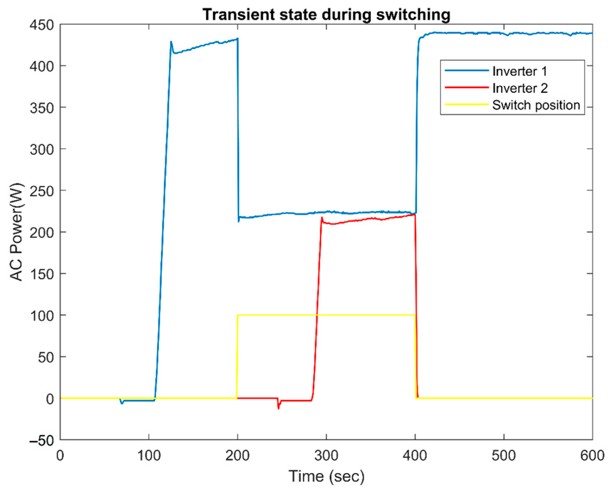
Figure 10 displays in blue and red traces the AC powers delivered by the two used inverters along a switch cycle. The switch position is indicated by the yellow trace and it is in accordance with the position indicated in Figure 7. A low level indicates position NC and a high level indicates NO position.
The two used SAS are programmed with a 220 W maximum power point and at t = 0 s only the inverter 1 (blue trace) is connected to the SAS. As can be seen, the inverter control system needs a period to perform some internal tests, the grid synchronization, and start proper operation.
At t = 200 s the switch is activated and the PV generator is divided between the two inverters. The output power of inverter 1 (blue trace) decreases in half and the controller of inverter 2 starts the turn-on cycle. After the initialization period, the output power of inverter 2 (red trace) increases and reaches the proper value, practically equal to the inverter 1 output power. As can be deduced from the obtained data, the transient period needed by the inverters to start the proper operation is about 95 s.
Finally, at t = 400 s, the switch is deactivated and inverter 2 becomes inactive. All the PVG is connected to inverter 1 and the transitory operation in this case is very short because it only depends on the operation of the implemented MPPT algorithm.
The transient previously described during the switch-on cycle has two main consequences that are necessary to consider:
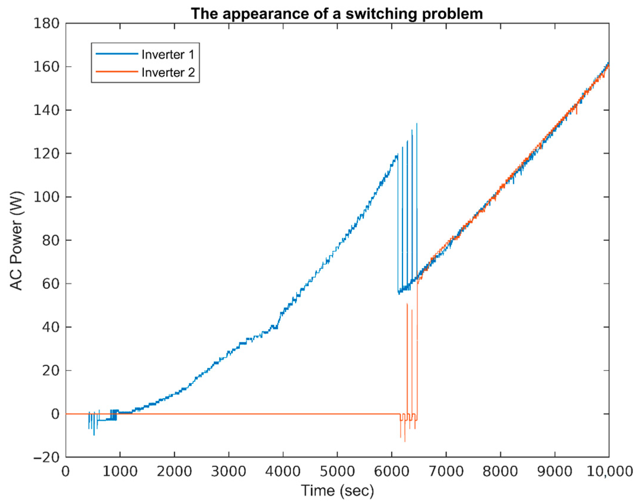
- Multiple switching around the power thresholds.
Figure 11 shows multiple switching within a short period. To address this issue, defining a margin or hysteresis band around the power threshold is proposed. In this regard, instead of using a specific value, the switching logic considers an upper limit and a lower limit. For instance, in our case, the lower power is PUD low = 95 W and the higher one is PUD high = 110 W. The results presented in the next sections provide evidence that this method is indeed effective and useful in preventing multiple switching operations around the power threshold levels.
- Power losses during the switching operation.
As can be seen in Figure 10, during the 95 s needed by one inverter to start the proper operation, some losses of power appear. In this period, only one inverter sends energy to the grid and the power lost is equal to PUD/2 or PUG.
As is presented previously, the tests performed use a threshold practically equal to PUD = 110 W, and, as a consequence, the energy losses (Elost) in each switch turn-on operation can be estimated using Equation (10).
6. Obtained Results
To evaluate and contrast the performance of reconfigurable and non-reconfigurable photovoltaic systems, several emulations have been performed simulating different meteorological conditions. Conditions similar to sunny, cloudy, and partly sunny days have been considered.
There are unlimited possibilities for irradiance patterns in different weather conditions, so it is impossible to emulate every situation. The choice of the irradiance profile used has been based only on energy criteria since this research work tries to evaluate the energy gains in reconfigurable PV systems when the PV inverters operate in low-load conditions.
The power output of the inverters on a “sunny day” is higher than the reconfiguration threshold most of the time, being lower than the reset threshold only during the first and last part of the day. This means that most of the time PV inverters do not operate in low-load conditions. On the other hand, the power output of the PV inverters on a “cloudy day” is lower than the reconfiguration threshold throughout the day and, consequently, the inverters always operate in low-load conditions.
In the case of irradiance and ambient temperature data, websites such as SoDa [50] offer valuable information based on the desired location and minute-by-minute data series. To obtain a per-second dataset to perform a real time emulation, data interpolation is performed as part of the emulation process. Additionally, the zero values of irradiance at the start and end of the day are removed in an effort to reduce the emulation time. Figure 12 depicts a plot of the used irradiance data.
The value of the irradiation data, expressed in W/m2, used for the three types of days considered is obtained by scaling the series shown in Figure 12.
This alternative has been chosen because the expected behavior of reconfigurable PV systems, when compared to non-reconfigurable systems, does not depend greatly on the irradiation profile used.
6.1. Sunny Day
A sunny day is characterized by high irradiance levels at midday and typically only requires two switching actions when considering a reconfigurable system. The initial switch action involves the PVG division when the irradiance reaches the PUD high threshold, and the second switch action involves the PVG grouping when the power diminishes and falls below the PUD low threshold.
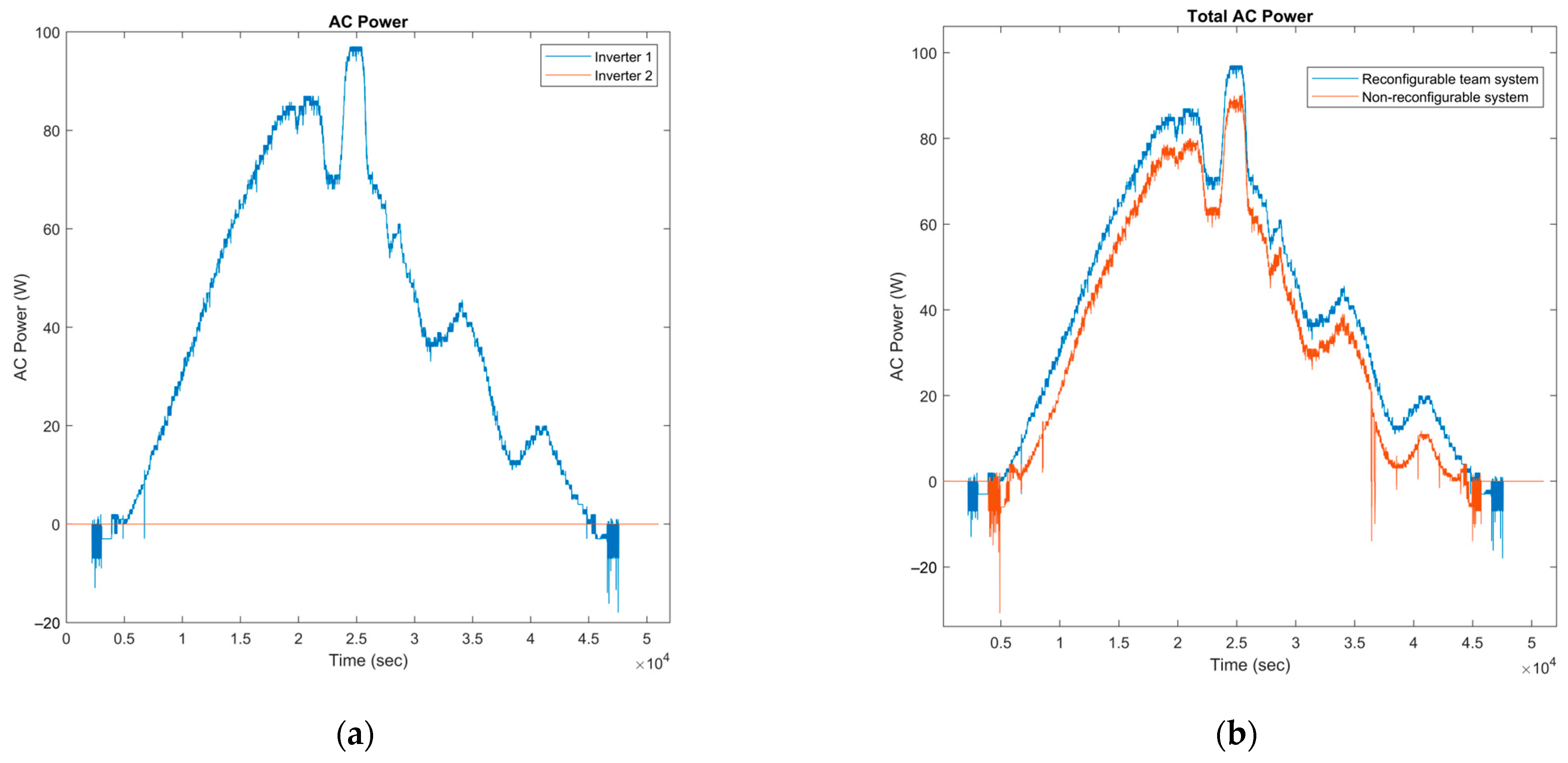
Figure 13 shows the power supply to the grid when a reconfigurable team system and a non-reconfigurable system are tested. Figure 13a shows the output power of the two inverters used in a reconfigurable team system. Figure 13b shows the output power of the non-reconfigurable system (red trace) and the output power of the reconfigurable team system (blue trace), the latter obtained as the sum of the output powers of the two inverters used.
As depicted in Figure 13a, initially, one of the team system inverters is utilized. However, once the threshold is reached, the second inverter is added (PVG division). At the end of the period, when the power is lower than the threshold, the reverse action of grouping takes place. As is expected, a small drop at the first switching point can be observed in the total AC power. This power loss can be seen in Figure 13b as a small glitch and in more detail in Figure 13c.
As seen in Figure 13c,d, the non-reconfigurable and reconfigurable systems demonstrate distinct performances in the two regions where the power remains below the threshold. Throughout this period, the reconfigurable system operates with a single inverter, while the non-reconfigurable system operates with both inverters. It can also be observed that the reconfigurable system delivers more power to the grid, showing greater efficiency in low-load conditions.
The energy supplied to the grid by the two tested systems is calculated from the instantaneous power data recorded by the PC used in the system. The power curves are numerically integrated using MATLAB and the results obtained are presented in Table 3. As discussed in the previous section, the last column represents the energy lost from generation during switching, as can be seen, the reconfigurable (team) system generates slightly more power than the fixed system.
6.2. Cloudy Day
In this study, a cloudy day is defined as a day in which, due to various factors including cloudiness, the amount of irradiance is so low that the power delivered by the system does not reach the PUD threshold.
As in the previous case, Figure 14 shows the power supply to the grid when a reconfigurable team system and a non-reconfigurable system are tested. Figure 14a shows the output power of the two inverters used in a reconfigurable team system. Figure 14b shows the output power of the non-reconfigurable system (red trace) and the output power of the reconfigurable team system (blue trace).
Figure 14a proves that the configurable system utilizes only one inverter during the whole day to increase the efficiency of the system. To facilitate the comparison, the AC powers of both non-reconfigurable and reconfigurable systems are shown in Figure 14b. As anticipated, the reconfigurable system demonstrates a higher power output during the day. This is because the two inverters used in the non-reconfigurable system operate under low-load conditions throughout the day.
The power supply to the grid in both cases is calculated numerically and it is shown in Table 4. Reviewing the obtained results, it can be concluded that on a cloudy day, the reconfigurable system exhibits a more significant energy efficiency.
6.3. Partially Sunny Day
A partly sunny day is characterized as a day in which, owing to various factors, the amount of radiation fluctuates, causing the power delivered by the system to exceed or fall below thresholds multiple times. Consequently, on a partly sunny day, configurable systems perform more switching operations compared to sunny days.
Figure 15 shows the power supply to the grid when a reconfigurable team system and a non-reconfigurable system are tested. Figure 15a shows the output power of the two inverters used in the reconfigurable team system, and Figure 15b shows the output power of the non-reconfigurable system (red trace) and the output power of the reconfigurable team system (blue trace).
As depicted in Figure 15a, the switching action has occurred four times. Following the conditions, the second inverter is introduced to the circuit in two stages and subsequently removed. Additionally, Figure 15b presents a comparison of the two systems in terms of delivered AC power. The reconfigurable system demonstrates better performance in sections below the PUD threshold.
The power supply to the grid in this case is calculated and presented in Table 5. Although the difference in energy delivered between the two systems is not as substantial as on a cloudy day, it is still significant. However, the last column of the table reveals a higher power loss due to the higher number of switching actions.
7. Discussion
MIX (or Multimaster) and team PV inverters were introduced by some manufacturers in the first decade of the 2000s to improve efficiency when central PV inverters operate under low-load conditions. This expected improvement in efficiency is highlighted in the technical documentation of these inverters, but there have been few published research studies on these topologies.
The lack of published studies can be understood in the case of MIX inverters due to the complexity of their design since it is based on the parallel operation of several inverters. In this topology, one inverter assumes the role of the leader device, and the remaining inverters are considered follower devices. Only the leader inverter implements an MPPT algorithm of the PVG, and the control of the MIX system must guarantee the correct distribution of energy between all inverters operating in parallel.
This topology is impossible to implement using conventional PV inverters because they must operate in a coordinated way, thus increasing the control complexity.
On the other hand, the lack of publications related to the team topology is less expected, since it can be implemented using conventional and commercial PV inverters. In this case, all active inverters have to implement an MPPT algorithm, and the power flow between the active PV inverters is directed using controlled switches.
In any case, the simulations performed of these two topologies of reconfigurable PV systems confirm that they have greater energy efficiency than those based on non-reconfigurable topologies. Furthermore, the tests carried out in this work on a PV system based on a team topology also confirm the higher energy efficiency initially assumed. In this regard, Table 6 presents an overview of results obtained from the emulations performed in this work.
According to the data obtained, days with low irradiance levels (always lower than the reconfiguration power threshold value) demonstrate greater increases in energy production when the reconfigurable system is considered.
Based on the tests carried out and the data obtained, it is practically impossible to make an accurate estimate of the increase in energy efficiency that can be obtained during one year if reconfigurable PV systems are used.
To perform this estimation, it would be necessary, among others, to have information on the daily weather in the considered location, and a representative irradiance profile should also be defined for each possible type of day. These issues define future lines of research in the field of reconfigurable photovoltaic systems, and they will be addressed in the future.
8. Conclusions
This work deals with some aspects related to the sizing ratio (RS) of GCPV systems and the relationship of this parameter with the available power at the output of the PVG. Additionally, the optimum value of the sizing ratio (RS OPT) of a GCPV non-reconfigurable system was defined as the one that maximizes the yearly energy efficiency (ηE) in the considered systems. A procedure to determine this optimum value has been presented. This procedure will be adapted to address the determination of RS in reconfigurable GCPV systems.
Systems with adjustable RS have been defined, differentiating between systems that adjust the RS value by modifying the rated power of the energy-processing subsystem used at each moment (called MIX or Multimaster systems), and systems that adjust the RS value by modifying the nominal power of the PVG connected to each energy-processing system (called team-based systems).
This presented work addresses issues related to the design of reconfigurable photovoltaic systems based on the team concept and the required control. An experimental setup for testing GCPV systems based on the team concept is described. A set of emulation tests for the characterization of these systems are described, and the obtained results are presented.
The results obtained from conducted emulations demonstrate that the reconfigurable systems exhibit superior performance on the defined as “cloudy” and “partly sunny” days when compared with non-reconfigurable systems. However, on the defined as “sunny” days, a slight variation in the energy generation is observed.
The notable variation observed in the energy production on “cloudy” and “partly sunny” days suggests that the utilization of team systems in regions characterized by low average irradiance would be advisable. Conversely, the marginal gain obtained in the results during a “sunny” day emulation indicates that employing the team system in areas with exceptionally high average irradiance may not substantially affect the system’s energy efficiency and, as a consequence, its utilization is not advisable.
Author Contributions
Conceptualization, G.V.-Q. and R.A.; methodology, G.V.-Q.; software, R.A.; validation, G.V.-Q. and R.A.; formal analysis, G.V.-Q.; investigation, G.V.-Q. and R.A.; resources, R.A.; data curation, R.A.; writing—original draft preparation, R.A.; writing—review and editing, G.V.-Q. and R.A. All authors have read and agreed to the published version of the manuscript.
Funding
The authors would like to thank the Spanish Ministerio de Ciencia, Innovación y Universidades (MICINN)—Agencia Estatal de Investigación (AEI) by project PID2022-138631OB-I00. Grant PID2022-138631OB-I00 funded by MICIU/AEI/10.13039/501100011033 and by “ERDF/EU”.
Institutional Review Board Statement
Not applicable.
Informed Consent Statement
Not applicable.
Data Availability Statement
All data generated or analyzed during this study are included in this article. All data included in this study are available upon request by contact with the corresponding author.
Conflicts of Interest
The authors declare no conflicts of interest.
References
- European Commission. In Focus: Reducing the EU’s Dependence on Imported Fossil Fuels. Brussels. 20 April 2022. Available online: https://commission.europa.eu/news/focus-reducing-eus-dependence-imported-fossil-fuels-2022-04-20_en (accessed on 8 March 2024).
- BP p.l.c. Statistical Review of World Energy 2022. July 2023. Available online: https://www.bp.com/en/global/corporate/energy-economics/webcast-and-on-demand.html#stats-review-archive (accessed on 8 March 2024).
- International Renewable Energy Agency (IRENA). Renewable Capacity Statistics 2022; IRENA: Masdar City, United Arab Emirates, 2022; ISBN 978-92-9260-428-8. Available online: https://www.irena.org/publications/2022/Apr/Renewable-Capacity-Statistics-2022 (accessed on 8 March 2024).
- Kibria, M.F.; Elsanabary, A.; Tey, K.S.; Mubin, M.; Mekhilef, S.A. Comparative Review on Single Phase Transformerless Inverter Topologies for Grid-Connected Photovoltaic Systems. Energies 2023, 16, 1363. [Google Scholar] [CrossRef]
- Tanrioven, M. Photovoltaic Systems Engineering for Students and Professionals: Solved Examples and Applications; CRC Press: Boca Raton, FL, USA, 2023; ISBN 978-1000936636. [Google Scholar]
- National Renewable Energy Laboratory (NREL). Champion Photovoltaic Module Efficiency Chart. Available online: https://www.nrel.gov/pv/module-efficiency.html (accessed on 8 March 2024).
- Fraas, L.M.; O’Neill, M.J. Low-Cost Solar Electric Power; Springer International Publishing: Cham, Switzerland, 2023; ISBN 978-3031308123. [Google Scholar]
- Camps, X.; Velasco, G.; de la Hoz, J.; Martín, H. Contribution to the PV-to-inverter Sizing Ratio Determination Using a Custom Flexible Experimental Setup. Appl. Energy 2015, 149, 35–45. [Google Scholar] [CrossRef]
- Hazim, H.I.; Baharin, K.A.; Gan, C.K.; Sabry, A.H.; Humaidi, A.J. Review on Optimization Techniques of PV/Inverter Ratio for Grid-Tie PV Systems. Appl. Sci. 2023, 13, 3155. [Google Scholar] [CrossRef]
- Wang, H.X.; Muñoz-García, M.A.; Moreda, G.P.; Alonso-García, M.C. Optimum inverter sizing of grid-connected photovoltaic systems based on energetic and economic considerations. Renew. Energy 2018, 118, 709–717. [Google Scholar] [CrossRef]
- Omar, M.A.; Mahmoud, M.M. Improvement Approach for Matching PV-array and Inverter of Grid Connected PV Systems Verified by a Case Study. Int. J. Renew. Energy Dev. 2021, 10, 687–697. [Google Scholar] [CrossRef]
- Zidane, T.E.K.; Zali, S.M.; Adzman, M.R.; Tajuddin, M.F.N.; Durusu, A. PV array and inverter optimum sizing for grid-connected photovoltaic power plants using optimization design. J. Phys. Conf. Ser. 2021, 1878, 012015. [Google Scholar] [CrossRef]
- Sulaiman, S.I.; Rahman, T.K.A.; Musirin, I.; Shaari, S. Sizing grid-connected photovoltaic system using genetic algorithm. In Proceedings of the IEEE Symposium on Industrial Electronics and Applications (ISIEA), Langkawi, Malaysia, 25–28 September 2011; pp. 505–509. [Google Scholar]
- Sulaiman, S.I.; Rahman, T.K.A.; Musirin, I.; Shaari, S.; Sopian, K. An intelligent method for sizing optimization in grid-connected photovoltaic system. Sol. Energy 2012, 86, 2067–2082. [Google Scholar] [CrossRef]
- Omar, A.M.; Shaari, S. Sizing verification of photovoltaic array and grid-connected inverter ratio for the Malaysian building integrated photovoltaic project. Int. J. Low-Carbon Technol. 2009, 4, 254–257. [Google Scholar] [CrossRef]
- Hussin, M.Z.; Omar, A.M.; Zain, Z.M.; Shaari, S. Sizing ratio of inverter and PV array for a-Si FS GCPV system in Malaysia’s perspectives. In Proceedings of the IEEE Control and System Graduate Research Colloquium (ICSGRC), Shah Alam, Malaysia, 16–17 July 2012; pp. 88–93. [Google Scholar]
- Kil, A.J.; van der Weiden, T.C.J. Performance of modular grid connected PV systems with undersized inverters in Portugal and the Netherlands. In Proceedings of the IEEE 1st World Conference on Photovoltaic Energy Conversion, Waikoloa, HI, USA, 5–9 December 1994; Volume 1, pp. 1028–1031. [Google Scholar]
- Omer, S.A.; Wilson, R.; Riffat, S.B. Monitoring results of two examples of building integrated PV (BIPV) systems in the UK. Renew. Energy 2003, 28, 1387–1399. [Google Scholar] [CrossRef]
- Islam, V.; Woyte, A.; Belmans, R.; Nijs, J. Undersizing inverters for grid connection—What is the optimum? In Proceedings of the PV in Europe, Rome, Italy, 7–11 October 2002; pp. 780–783. [Google Scholar]
- Gonzalez, R.; Jimenez, H.R.; Huacuz, J.M. Voltage and power ratio effects of grid-connected PV Plant’s operation on the performance ratio and total system efficiency. In Proceedings of the 3rd International Conference on Electrical and Electronics Engineering, Veracruz, Mexico, 6–8 September 2006; pp. 1–4. [Google Scholar]
- Macedo, W.N.; Zilles, R. Operational results of grid-connected photovoltaic system with different inverter’s sizing factors (ISF). Prog. Photovolt. Res. Appl. 2007, 15, 337–352. [Google Scholar] [CrossRef]
- Abo-Khalil, A.G.; Sayed, K.; Radwan, A.; El-Sharkawy, I.A. Analysis of the PV system sizing and economic feasibility study in a grid-connected PV system, Case Studies. Case Stud. Therm. Eng. 2023, 45, 102903. [Google Scholar] [CrossRef]
- Díaz-Bello, D.; Vargas-Salgado, C.; Águila-León, J.; Lara-Vargas, F. Methodology to Estimate the Impact of the DC to AC Power Ratio, Azimuth, and Slope on Clipping Losses of Solar Photovoltaic Inverters: Application to a PV System Located in Valencia Spain. Sustainability 2023, 15, 2797. [Google Scholar] [CrossRef]
- da Silveira Brito, E.M.; Cupertino, A.F.; Pereira, H.A.; Mendes, V.F. Reliability-based trade-off analysis of reactive power capability in PV inverters under different sizing ratio. Int. J. Electr. Power Energy Syst. 2022, 136, 107677. [Google Scholar] [CrossRef]
- Chen, X.; Melia, J. Inverter size optimization for grid-connected concentrator photovoltaic (CPV) plants. In Proceedings of the 37th IEEE Photovoltaic Specialists Conference (PVSC), Seattle, WA, USA, 19–24 June 2011; pp. 991–993. [Google Scholar]
- Chen, S.; Li, P.; Brady, D.; Lehman, B. Determining the optimum grid-connected photovoltaic inverter size. Sol. Energy 2013, 87, 96–116. [Google Scholar] [CrossRef]
- Velasco, G.; Guinjoan, F.; Piqué, R.; Román, M.; Conesa, A. Simulation-based criteria for the power sizing of grid-connected PV systems. Int. Rev. Model. Simul. (I.RE.MO.S.) 2011, 4, 10. [Google Scholar]
- Burger, B.; Rüther, R. Inverter Sizing of Grid-connected Photovoltaic Systems in the Light of Local Solar Resource Distribution Characteristics and Temperature. Sol. Energy 2006, 80, 32–45. [Google Scholar] [CrossRef]
- Skoplaki, E.; Palyvos, J.A. Operating Temperature of Photovoltaic Modules: A Survey of Pertinent Correlations. Renew. Energy 2009, 34, 23–29. [Google Scholar] [CrossRef]
- Ross, R., Jr. Interface design considerations for terrestrial solar cell modules. In Proceedings of the 12th Photovoltaic Specialists Conference, Baton Rouge, LA, USA, 15–18 November 1976; pp. 801–806. [Google Scholar]
- Herteleer, B.; Kladas, A.; Chowdhury, G.; Catthoor, F.; Cappelle, J. Investigating methods to improve photovoltaic thermal models at second-to-minute timescales. Sol. Energy 2023, 263, 111889. [Google Scholar] [CrossRef]
- Nordmann, T.; Clavadetscher, L. Understanding temperature effects on PV system performance. In Proceedings of the 3rd World Conference on Photovoltaic Energy Conversion, Osaka, Japan, 11–18 May 2003; pp. 2243–2246. [Google Scholar]
- Martín-Chivelet, N.; Polo, J.; Sanz-Saiz, C.; Núñez Benítez, L.T.; Alonso-Abella, M.; Cuenca, J. Assessment of PV Module Temperature Models for Building-Integrated Photovoltaics (BIPV). Sustainability 2022, 14, 1500. [Google Scholar] [CrossRef]
- BasseyAsuquo, S.; Kingsley, U.M.; Constance, K. Empirical Performance and Parametric Analysis of Photovoltaic System in Uyo. Sci. Technol. Publ. (SCI & TECH) 2019, 3, 273–276. [Google Scholar]
- de Oliveira Santos, L.; de Carvalho PC, M.; de Oliveira Carvalho Filho, C. Photovoltaic Cell Operating Temperature Models: A Review of Correlations and Parameters. IEEE J. Photovolt. 2022, 12, 179–190. [Google Scholar] [CrossRef]
- Keddouda, A.; Ihaddadene, R.; Boukhari, A.; Atia, A.; Arıcı, M.; Lebbihiat, N.; Ihaddadene, N. Photovoltaic module temperature prediction using various machine learning algorithms: Performance evaluation. Appl. Energy 2024, 363, 123064. [Google Scholar] [CrossRef]
- Baumgartner, F.P.; Schmidt, H.; Burger, B.; Bründlinger, R.; Häberlin, H.; Zehner, M. Status and Relevance of the DC Voltage Dependency of the Inverter Efficiency. In Proceedings of the 22nd EU PVSEC, Milan, Italy, 3–7 September 2007. [Google Scholar]
- Velasco, G.; Martinez, H. Sizing Factor Considerations of Grid-Connected Photovoltaics Systems. In Solar Energy Systems: Progress and Future Directions; Nova Science Publishers, Inc.: New York, NY, USA, 2019; pp. 61–101. ISBN 978-1-53616-142-7. [Google Scholar]
- Mühlberger, T.; Wolfahrt, J. Modular System. Maximum Yield: Fronius MIXTM System Optimizes Yield. In Photovoltaic System Technology; Fronius International GmbH: Pettenbach, Austria, 2012. [Google Scholar]
- Utility Scale Solar Inverters; P.N. 0701-0006-14 10/13; Emerson Electric Co.: St. Louis, MO, USA, 2013.
- ABB Central Inverters. ULTRA-750/1100/1500—750 kW to 1560 kW. ABB. 2015. Available online: https://www.fimer.com/sites/default/files/ULTRA-EN-Rev%20E.pdf (accessed on 8 March 2024).
- Vacon 8000 Solar Inverter. A Driving Force in Solar Energy; DPD01502G; Vacon: Vaasa, Finland, 2012. [Google Scholar]
- Häberlin, H. Photovoltaics. System Design and Practice; Wiley: Hoboken, NJ, USA, 2012; ISBN 978-1119978381. [Google Scholar]
- Mertens, K. Photovoltaics. Fundamentals, Technology, and Practice; Wiley: Hoboken, NJ, USA, 2018; ISBN 978-1119401049. [Google Scholar]
- Jasper, A.; Blume, L.; Glowka, M. Sunny Family 2008/2009; SMA Solar Technology AG: Niestetal, Germany, 2008. [Google Scholar]
- Central Inverter SUNNY CENTRAL User Manual. SMA Solar Technology AG. 2020. Available online: https://files.sma.de/downloads/SC-BEN092751.pdf (accessed on 8 March 2024).
- Maranda, W.; De Mey, G.; De Vos, A. Optimization of the Master–Slave Inverter System for Grid–Connected Photovoltaic Plants. Energy Convers. Manag. 1998, 39, 1239–1246. [Google Scholar] [CrossRef]
- Sreekanth, S.; Joseph, X.F. PV System with Multimaster Technique Implemented String Inverters. In Advances in Automation, Signal Processing, Instrumentation, and Control; Springer: Berlin/Heidelberg, Germany, 2021; ISBN 978-981-15-8220-2. [Google Scholar]
- Spertino, F.; Corona, F.; Di Leo, P. Limits of Advisability for Master–Slave Configuration of DC–AC Converters in Photovoltaic Systems. IEEE J. Photovolt. 2012, 2, 547–554. [Google Scholar] [CrossRef]
- Solar Radiation and Meteorological Data Services. SoDa Website. Available online: https://www.soda-pro.com/ (accessed on 8 March 2024).
Figure 1.
Elements in a GCPV system based on PO configuration.

Figure 2.
Block-diagram of the simulation procedure utilized to obtain the RS OPT value.

Figure 3.
RS OPT value of a GCPV located in Brussels.

Figure 4.
MIX system based on three inverters to set the energy-processing subsystem. (a) Configuration used during periods of low energy production with a higher sizing ratio. (b) Configuration after exceeding a certain power threshold, with a lower sizing ratio than the previous configuration. (c) Configuration used during periods of greatest energy production. It has the lowest sizing ratio of the three possible configurations.

Figure 5.
The three available configurations and the corresponding RS value for a team GCPV system with n = 4. (a) Configuration used in periods of lower energy production with the highest value of sizing ratio. (b) Reconfiguration after exceeding a certain power threshold, which has a lower sizing ratio than the previous configuration. (c) Configuration used during the periods of greatest energy production with a smaller value of sizing ratio compared with the two previous configurations.

Figure 6.
Relationship between annual energy efficiency (ηE) and the number of basic PV generators (n) used in a team-based GCPV system of up to n = 8.
Figure 6.
Relationship between annual energy efficiency (ηE) and the number of basic PV generators (n) used in a team-based GCPV system of up to n = 8.

Figure 7.
Diagram of the experimental set used for a team-based GCPV system characterization.

Figure 8.
Experimental set used for a team-based GCPV system characterization.

Figure 9.
Efficiency curve characterization of the used inverters.

Figure 10.
Output power of the two used inverters along a one switch cycle.

Figure 11.
Multiple switching operation around the threshold level PUD.

Figure 12.
Irradiance values, expressed in arbitrary units, used for the systems emulation.

Figure 13.
Performance of non-reconfigurable (fixed) and reconfigurable (team) systems on a sunny day. (a) AC power delivered by two inverters in the reconfigurable system; (b) AC power delivered by fixed and team system; and (c,d) details of the performance difference between the two compared systems in low-load conditions.

Figure 14.
Performance of non-reconfigurable (fixed) and reconfigurable (team) systems on a cloudy day. (a) AC power delivered by the two inverters of the reconfigurable system; (b) AC power delivered by fixed and team systems.
Figure 14.
Performance of non-reconfigurable (fixed) and reconfigurable (team) systems on a cloudy day. (a) AC power delivered by the two inverters of the reconfigurable system; (b) AC power delivered by fixed and team systems.

Figure 15.
Performance of non-reconfigurable (fixed) and reconfigurable (team) systems on a partly sunny day. (a) AC power delivered by the two inverters of the reconfigurable system; and (b) AC power delivered by fixed and team systems.
Figure 15.
Performance of non-reconfigurable (fixed) and reconfigurable (team) systems on a partly sunny day. (a) AC power delivered by the two inverters of the reconfigurable system; and (b) AC power delivered by fixed and team systems.


Table 1.
k coefficients comparison according to three datasets.
| k0 | k1 | k2 | |
|---|---|---|---|
| Inverter 1 | 0.027444 | 0.096693 | 1.004568 |
| Inverter 2 | 0.026962 | 0.110187 | 0.999356 |
| Merged data | 0.027626 | 0.105882 | 1.000143 |
Table 2.
Power thresholds obtained from the three datasets obtained.
| (W) | (W) | |
|---|---|---|
| Inverter 1 | 53.76 | 107.52 |
| Inverter 2 | 53.43 | 106.85 |
| Merged data | 54.06 | 108.12 |
Table 3.
Calculated energies comparison of the two considered systems.
| Energy by First Inverter (Wh/Day) | Energy by Second Inverter (Wh/Day) | Total Energy (Wh/Day) | Switching Energy Losses (Wh/Switching) | |
|---|---|---|---|---|
| Fixed system | 2427.76 | 2431.56 | 4859.32 | - |
| Team system | 2487.43 | 2386.35 | 4873.78 | 1.10 |
Table 4.
Energetic evaluation of the two analyzed systems.
| Energy by First Inverter (Wh/Day) | Energy by second Inverter (Wh/Day) | Total Energy (Wh/Day) | Switching Energy Losses (Wh/Switching) | |
|---|---|---|---|---|
| Fixed system | 201.25 | 210.01 | 411.25 | - |
| Team system | 500.05 | - | 500.05 | - |
Table 5.
Energy comparison between the two examined system.
| Energy by First Inverter (Wh/Day) | Energy by Second Inverter (Wh/Day) | Total Energy (Wh/Day) | Switching Energy Losses (Wh/Switching) | |
|---|---|---|---|---|
| Fixed system | 272.00 | 279.58 | 551.58 | - |
| Team system | 546.45 | 82.36 | 628.81 | 2.10 |
Table 6.
Increase in the amount of energy delivered to the grid (absolute value) and energy gain (expressed in percentage).
Table 6.
Increase in the amount of energy delivered to the grid (absolute value) and energy gain (expressed in percentage).
| Sunny Day | Cloudy Day | Partly Sunny Day | |
|---|---|---|---|
| Increment of energy (Wh/day) | 14.47 | 88.80 | 77.23 |
| Energy gain | 0.3% | 21.6% | 14.0% |
Disclaimer/Publisher’s Note: The statements, opinions and data contained in all publications are solely those of the individual author(s) and contributor(s) and not of MDPI and/or the editor(s). MDPI and/or the editor(s) disclaim responsibility for any injury to people or property resulting from any ideas, methods, instructions or products referred to in the content. |
© 2024 by the authors. Licensee MDPI, Basel, Switzerland. This article is an open access article distributed under the terms and conditions of the Creative Commons Attribution (CC BY) license (https://creativecommons.org/licenses/by/4.0/).
Share and Cite
MDPI and ACS Style
Afzali, R.; Velasco-Quesada, G. Energy Efficiency Improvement in Reconfigurable Photovoltaic Systems: An Evaluation of Team Systems. Appl. Sci. 2024, 14, 3368. https://doi.org/10.3390/app14083368
AMA Style
Afzali R, Velasco-Quesada G. Energy Efficiency Improvement in Reconfigurable Photovoltaic Systems: An Evaluation of Team Systems. Applied Sciences. 2024; 14(8):3368. https://doi.org/10.3390/app14083368
Chicago/Turabian StyleAfzali, Roohollah, and Guillermo Velasco-Quesada. 2024. "Energy Efficiency Improvement in Reconfigurable Photovoltaic Systems: An Evaluation of Team Systems" Applied Sciences 14, no. 8: 3368. https://doi.org/10.3390/app14083368
Note that from the first issue of 2016, this journal uses article numbers instead of page numbers. See further details here.