Prediction of Railway Embankment Slope Hydromechanical Properties under Bidirectional Water Level Fluctuations

Abstract

Railway embankment slopes are exposed to natural hazards such as excess rainfall, floods, earthquakes, and lake water/groundwater level variations. These are generally considered during the design, construction, and maintenance periods of the embankment. In this study, combined laboratory test methods and a computational approach were applied to assess the effect of groundwater level changes on the railway embankment. The Plackett–Burman (PBD), Box–Behnken design response surface methodology (BBD-RSM), and an artificial neural network (ANN) were used to predict the behavior of the embankment soil hydromechanical properties to determine the integrity of the embankment as water level fluctuates under varied seasonal conditions. The results show that the seepage line is concave during the rising water level (RWL) period, and the railway slope’s static stability factor surges and then stabilizes. Further analysis found that the slope’s stability is largely affected by some of the hydromechanical properties of the soil embankment material, such as the internal friction angle (ϕ), soil density (ρ_s), and cohesion (c). The second-order interaction factors c x s, x s, and s² also affect the stability factor. It was observed that the four most sensitive parameters under both falling water level (FWL) and RWL conditions are ϕ, ρ_s, c, and rate of fall/rise in water level (H). The statistical evaluation of the RSM model produced R² values of 0.99(99) and 0.99, with MREs of 0.01 and 0.24 under both RWL and FWL conditions, respectively, while for ANN, they produced R² values of 0.99(99) and 0.99(98), with MRE values of 0.02 and 0.21, respectively. This study demonstrates that RSM and ANN performed well under these conditions and enhanced accuracy, efficiency, iterations, trial times, and cost-effectiveness compared to full laboratory experimental procedures.

1. Introduction

The exposure of embankment infrastructure to natural hazards is unavoidable [1]. This results in the instability of embankment slopes, which has increased in recent times due to human activities [2] and climate variability [3]. On a global scale, this problem poses a serious threat to the management and development of railway infrastructure and similar transportation networks [4]. Recently, the long-term performance of embankment slopes has become a focus of scrutiny [5,6]. The consequences of climate change have made rail infrastructure more vulnerable to water-related risks, such as floods [7], ponding, and fluctuations in water levels [8].

China has one of the most diversified hydrological systems in the world [9], with a complex network of rivers, such as the Yellow and Yangtze Rivers, as well as enormous lakes, such as Qinghai Lake and Dongting Lake. The area surrounding Dongting Lake (the study area), near the Nanhu railway embankment between Beijing and Guangzhou provinces, has been affected by the lake’s fluctuations (and resulting groundwater changes), resulting in multiple failures and constant repair. As a result, these situations not only accelerate embankment deterioration but also drive up rehabilitation and maintenance costs [10]. To address these challenges, several solutions have been used, including the placement of soil reinforcement techniques ranging from fibers and rock mixtures [11] to steel piling [12]. However, the control of traffic loads and the consequences of climate change have made these efforts persistently difficult [13]. Ensuring the long-term stability of embankment slopes under water level fluctuation requires advanced engineering solutions that could capture seasonal and long-term fluctuations while allowing for increased traffic demands at the same time [14,15]. An attempt to address these difficulties is crucial to ensuring the reliability and resilience of critical transportation systems [16]. Recent studies have stressed the relevance of incorporating soil hydromechanical parameters for evaluating the performance of embankment slope constructions under different geohazard conditions [17,18,19,20]. Using the bibliometric tool VOSviewer 1.6.19 to analyze previous studies from the Scopus database revealed a noticeable trend in slope stability analysis under changing water levels and limited work on sensitivity and optimization of slope stability factors (see Figure 1).

In addition to external influences, the physical properties of the material structure are internal elements that play an important role in slope stability, as the changes in saturation states of the soil due to seepage fields impact both local and overall slope stability [17,21]. Additionally, groundwater table variations could have considerable impact on the slope stability due to its time domain [22,23]. Another way to improve the performance of railway embankment slopes is to examine the quantitative relationships between parameters regulating safety coefficients [24]. Technically, this requires examining the effect of changes in each hydromechanical parameter on the safety factor and knowledge about their dominating roles in stability analysis [25]. This is critical for developing appropriate mitigation strategies and control guidelines to minimize instability [26]. Unfortunately, water level changes in railway slope stability is a subject that has received little attention [27]. Some studies advise that for long-term performance and a robust railway system, sensitivity assessments for each parameter of the railway slope under bidirectional water levels are critical [28]. Zhou [17] investigated the sensitivity of variables such as unit weight, internal friction angle, water level, and cohesiveness on the slope stability factor of safety. Using the tree-augmented naive Bayes (TANB) approach, Ahmad [29] studied the impacts of parameters such as pore–pressure ratio, internal friction angle, cohesion, slope angle, and unit weight on the stability coefficient. Using an artificial neural network, Abdalla [30] investigated the effects of variables such as internal friction angle, cohesiveness, slope height, and unit weight on the stability factor. Tao [31] used a support vector machine (SVM) [32] to evaluate slope parameters. Hu [33] assessed the sensitivity of unit weight, cohesiveness, and internal friction angle to the slope stability factor of safety using partial Spearman rank (PSS) correlation coefficients.

Zhou et al. [17] used reliability coefficients with cohesion and internal friction angle as components, following other studies of sensitivity analysis for embankment slope parameters [34,35,36,37]. However, fluctuating water levels coupled with the static train loads found a sensitivity analysis of railway embankment slopes complicated. To understand their interactions and the influence of input factors on the response variable, it is critical to build a trustworthy and obvious relationship between output and input variables [38]. Existing studies have concentrated on individual hydromechanical parameters of the soil or external factors (rainfall, water level fluctuation, etc.), with little focus on interactions and sensitivity to railway embankment slopes. Ignoring factor interactions may not accurately depict the nonlinear relationships between components and the slope’s response factor, which is a key drawback in past research. Hence, this study aimed to evaluate the connection between external and internal factors and their impact on the stability of the railway embankments while considering the coupled impacts of the static load stress under fluctuating water levels. To integrate this concept, a method for performing thorough and reliable coupled static stress and seepage sensitivity analyses on railway slopes was developed. Emerging artificial intelligence approaches, such as fuzzy logic (FL), ANN [39,40] and gene expression programming (GENXPRO) are regarded as robust and reliable for developing slope stability models, even without prior knowledge of the seepage and stress fields within the railway embankment slope environment. Several strategies for improving the accuracy of ANN model predictions have been proposed [29], with the back-propagation algorithm (BP) standing out as particularly effective [41]. To achieve these objectives and establish the integration of both internal and external embankment stability controlling factors, both artificial neural network (ANN) and Box–Behnken design (BBD-RSM) models were selected due to their good precision in the field of civil engineering [41,42].

2. Materials and Methods

2.1. The Plackett–Burman and BBD-RSM Experiment Design

The Plackett–Burman design (PBD) is a powerful tool for analyzing variables and identifying critical factors [43]. It achieves this by examining a large number of variables within a small number of experiments. The BBD-RSM embedded in the Design-Expert 13.0.0 program [44] was used to simulate and assess the interactions of the contributing variables selected by PBD during stability coefficient determination [44]. Hence, the BBD for three independent parameters (cohesion (c), elastic modulus (E), water level rate of change (v), internal friction angle (ϕ), train static load (L), infiltration coefficient (k_s), soil unit weight (ρ_s), elevation of fluctuating water level (H), Poisson’s ratio (v), residual moisture content (θ_r), and van Genuchten fitting parameters (n, m, and α)) were used to determine the effect on earth material embankment stability. The following equation is the baseline mathematical relationship used by BBD [45]:

$$Y={\beta }_0+{{\displaystyle \sum }}_{i=1}^k {\beta }_0 X_i+{{\displaystyle \sum }}_{i=1}^k {\beta }_{ii} {X_{ii}}^2+{{\displaystyle \sum }}_{i=1}^k {\beta }_{ij} X_i{X}_j$$

(1)

where Y is the predicted response; β₀ is constant; and β_i, β_ii, and β_ij are the linear, quadratic, and interaction coefficients. Finally, X_i and X_j are the coded values of independent parameters.

2.2. The Artificial Neural Network (ANN) Model and Its Importance

Buscema [46] says it is important to give a clear definition of the interlayer as the point where two successive layers meet, where the connection weights spin across the neurons of the leading layer. The MLP network under analysis contains X interlayers.

For interlayer $x\in \left\{1,2,3,4, \dots \dots X\right\}$, there are $J_x$ of nodes and $J_x\times J_{x-1}$ connection links with weights $W\in R^{J_x\times J_{x-1} }$, where $J_x$ and $J_{x-1}$ are the numbers of nodes (including thresholds) in interlayers $x$ and $x-1$, respectively. A connection weight is defined as ${W_{k,i}}^x$ if it resides in interlayer $x$ and connects node $k$ of interlayer $x$ with $i$ of lower (preceding) internode layer $x-1$ (node i is the source node, and node k is the destination node). In any interlayer x, a typical neuron k integrates the signals, $y_k$, imposing onto it and result to a net effect, ${ϵ}_k$, giving to linear neuron dynamics given as follows:

$${{ϵ}_k}^x={{\displaystyle \sum }}_{i=1}^{X_{l-1}}{w_{k,i}}^x{x_i}^{x-1}$$

(2)

The corresponding activation, y_k^x, of the neuron is determined using a transfer function, $\sigma$, that converts the total signal into a real number from a bounded interval, as follows:

$${y_k}^x=\sigma {{ϵ}_k}^x=\sigma {{\displaystyle \sum }}_{i=1}^{X_{l-1}}{w_{k,i}}^x{x_i}^{x-1}$$

(3)

One general function used in BP is the basic continuous sigmoid, as follows:

$$\sigma \left(ϵ\right)=\frac{1}{1+e^{-ϵ}}$$

(4)

where $\infty >ϵ>-\infty$ and $1.0\ge \sigma \ge 0.0$ are used for all nodes to compute the activation. For the input nodes, the activation is purely the raw input.

Iteration was used to construct network outcomes (predicted values) that closely matched the actual values by modifying input weights, layer weights, and biases. The datasets were separated into training, testing, and cross-validation sets to avoid over-parameterization and over-training [47]. The data from 17 experimental runs were randomly divided into three sets in the SRFI model for training (50%), testing (25%), and validation (25%). Similarly, the SRF2 model data from 30 experimental runs was divided into training (70%), testing (15%), and validation (15%). The research evaluated different ANN model topologies from 3 to 10 neurons to see which produced the highest correlation of coefficients (R²) and the lowest mean-square error (MSE) and root mean-square error (RMSE) for the training, test, and validation datasets.

2.3. Models and Evaluation Criteria for ANN and BBD-RSM

The significance and performance of the ANN and BBD-RSM models were assessed using the following statistical performance indices: coefficient of determination (R²), mean relative error (MRE), and roots mean-square error (RMSE), as follows:

$$R^2=1-\left(\frac{{{\displaystyle \sum }}_{i=1}^n{\left(S_i-F_i\right)}^2}{{{\displaystyle \sum }}_{i=1}^n{\left(F_i\right)}^2}\right)$$

(5)

$$RMSE=\sqrt{\frac{1}{n}{\displaystyle \sum }_{i=1}^n{\left(S_i-F_i\right)}^2}$$

(6)

$$MRE\left(\%\right)=\frac{1}{n}{\displaystyle \sum }_{i=1}^n\left|100\frac{S_i-F_i}{S_i}\right|$$

(7)

where, $S_i$ and $F_i$ represent the actual parameter and predicted parameter values, respectively, as determined by the ANN and BBD-RSM models, and n denotes the total sample size or number of parameters.

2.4. Study Area Overview

The railway embankment examined in this study is the K1430 + 110 of the Beijing-Guangzhou Railway in Yueyang City, Hunan province; 113°05′00.46″ E, 29°20′48.66″ N. This area has complex geological and hydrological conditions. Hydrologically, the area has a humid subtropical climate with variable rainfall and high humidity. The region experiences monsoon rains, which can cause flash floods and landslides [48]. The K1430 + 110 stretch of the Beijing-Guangzhou Railway embankment in Figure 2 is near Dongting Lake, one of China’s largest freshwater lakes and a vital hydropower and irrigation resource. Flooding is common due to its low-lying topography and proximity to Dongting Lake and the Yangtze River (Figure 2).

This research compared BBD-RSM and ANN methods and proposed a related seepage-stress field-based sensitivity analysis strategy. The objective was to evaluate how various elements and their interactions affect railway embankment slope stability under changing lake water (and subsequent seepage groundwater) levels. A section of the Beijing-Guangzhou railway embankment slope at Nanhu, Hunan Province, China, was used to demonstrate the methodology. The main objective was to evaluate the sensitivity of each significant element and their interaction terms for the railway embankment slope stability coefficient of safety.

2.5. Modeling Approach

Physical parameters of the railway embankment slope were obtained using laboratory testing. A cross-section of the railway embankment slope (Figure 2c) [48] and lake water level measurements were collated.

A 2D finite element model of the railway embankment slope was produced using the soil material parameters from experimental data using GeoStudio 2012 software [49]. Currently, there is no information on groundwater/surface water interaction or lag times for the study area. Therefore, an instantaneous change in pore water pressure with variations in lake levels was employed to establish the model boundary conditions for both rising (0.1 m/day) and falling (0.2 m/day) scenarios. Scenarios 1 and 2 are as follows: increasing water (53.5 m to 71.2 m and 53.5 m to 58 m) used historical field data of the lake water levels. These were observed to be critical within 20 days in the summer and autumn, and hence, seepage analysis was conducted for 20 days under various drawdown scenarios. Previous research shows that water level and antecedent precipitation changes most affect slope stability after 5 days [50,51,52].

The Plackett–Burman experimental design is used to screen nine parameters affecting railway embankment slope stability; the most critical parameters were chosen, and minor factors were excluded. The BBD-RSM test design evaluated the main and interaction effects of selected significant factors from the Plackett–Burman test. Components with considerable sensitivity to the railway slope stability coefficient were identified. The BBD-RSM dataset was used to build an ANN model using JMP Pro 15.0 software [48]. Finally, BBD-RSM and ANN findings were compared to assess their stability factor sensitivity analysis performance.

In this study, nine external and internal elements affecting railway embankment stability were screened. Two unique levels were selected by the One Factor at a Time process for each factor.

Table 1. Experimental levels for nine parameters using Plackett–Burman and BBD-RSM.

Factor Level	v (m/s)	ρs (kg/m3)	c (Kpa)	φ (°)	L (KN)	κs (m/s)	μ	E (Mpa)	H (m)
+	0.22	2090	15.4	37.4	143	5.83 × 10−6	0.33	25.85	18.7
0	0.2	1900	14	34	130	5.30 × 10−6	0.3	23.5	17.0
-	0.18	1710	12.6	30.6	117	4.77 × 10−6	0.27	21.15	15.3

show the factors analyzed and their greater (+) and lower (−) values. A full matrix of a normal 12-run PBD (

Table 2. Results and scenarios of Plackett–Burman analysis of nine criteria for rising and falling water level.

Iterations	Plackett–Burman Analysis of Nine Criteria for Rising Water Level										Plackett–Burman Analysis of Nine Criteria for Falling Water Level
	H	v	k	c	ϕ	µ	E	ρs	L	SRF Rising	H	v	k	c	ϕ	µ	E	ρs	L	SRF Falling
ID
SR 1	+	−	−	−	+	+	+	−	+	2.155	+	+	−	+	+	−	+	−	−	1.986
SR 2	+	+	−	+	−	−	−	+	+	2.066	+	+	−	+	−	−	−	+	+	1.782
SR 3	+	−	+	−	−	−	+	+	+	1.827	−	−	−	−	−	−	−	−	−	1.78
SR 4	−	−	−	−	−	−	−	−	−	1.825	+	−	−	−	+	+	+	−	+	1.931
SR 5	−	+	−	−	−	+	+	+	−	1.891	+	+	+	−	+	+	−	+	−	1.852
SR 6	−	+	+	−	+	−	−	−	+	2.031	−	+	−	−	−	+	+	+	−	1.703
SR 7	−	−	+	+	+	−	+	+	−	2.28	−	+	+	−	+	−	−	−	+	1.916
SR 8	+	−	−	−	+	+	+	−	+	2.131	+	−	+	+	−	+	−	−	−	1.846
SR 9	+	−	+	+	−	+	−	−	−	2.07	−	−	−	+	+	+	−	+	+	2.011
SR 10	−	+	+	+	−	+	+	−	+	1.947	+	−	+	−	−	−	+	+	+	1.681
SR 11	+	+	−	+	+	−	+	−	−	2.156	−	+	+	+	−	+	+	−	+	1.826
SR 12	+	+	+	−	+	+	−	+	−	2.13	−	−	+	+	+	−	+	+	−	2.009

) was constructed using Minitab 19.0 [17].

3. Results and Discussion

3.1. Parameter Screening with Plackett–Burman (PBD) and RSM Modeling

The global perturbation analysis method examined parameter influences from external and internal sources. Therefore, a screening strategy was used to choose the most sensitive embankment stability coefficient values, followed by an assessment of their total sensitivity. The initial screening of the 14 factors affecting railway embankment stability used PBD by Minitab 19.0 [17]. These factors include cohesion (c), elastic modulus (E), water level rate of change (v), internal friction angle (ϕ), train static load (L), infiltration coefficient (k_s), soil unit weight (ρ_s), elevation of fluctuating water level (H), Poisson’s ratio (v), residual moisture content (θ_r), and van Genuchten fitting parameters (n, m, and α). Zhang [17] found that θ_s, n, m, α, and θ_r have little effect on earth material embankment stability and were assumed to be negligible.

This study only examined L, v, ρ_s, c, k_s, ϕ, E, H, and ν. Each variable was tested at two independent levels, with the lower level (−1) set to drop by 10% from the baseline basic working norm and the higher level (+1) set to grow by 10% [17]. Table 1 shows a 20% difference between the higher and lower levels. A probability value (p-value) below 0.05 in the statistical analysis showed a significant influence on the railway embankment stability factor, guiding the PBD test factor selection, as shown in Table 2. These parameters’ primary effects were assessed using PBD and were further evaluated for main effects using BBD-RSM.

The normalized effects show that when rising lake water levels impact the railway slope, the impact of each influencing parameter is ranked in ascending order: µ < E < v < Ks < H < L < c< ρ_s< ϕ. Interestingly, c, ρ_s, and ϕ greatly impact the global static stability and safety factor of the railway embankment slope. E, v, Ks, H, and L are less important. PBD results show that when water levels drop, the sensitivity of each parameter is classified as follows: E < µ < v < K_s < L < ρ_s < H < c < ϕ. This indicates that ϕ, c, H, and ρ_s greatly affect the railway slope’s global static stability and safety factor. The parameters E, v, K_s, L, and µ have minimal impact on the global static stability of the railway slope and its factor of safety. A preliminary analysis shows that the mechanical properties (ϕ, c, and ρ_s) of the railway slope are affected through its global stability and safety factor during varying water levels. Train static loading does not affect the global static slope factor of safety, but it is stronger when water levels rise than decline. The soil coefficient of permeability, K_s, is less sensitive to the railway slope’s global static stability safety coefficient, possibly due to embankment compaction rates [17].

In addition, the seepage flux (K_s, H, and v) sensitiveness on the railway slope’s static stability coefficient is greater with falling water levels than with rising levels. The lake’s fast water level variations may explain this (assuming instantaneous pore water pressure response). Thus, the railway embankment slope seepage field characteristics (K_s, H, and v) will need to be monitored for long-term sensitivity. Based on the standardized effects chart, three of the most influential components for the increasing water level scenario and four for the dropping water level scenario were selected for BBD-RSM analysis.

The variables H, ρ_s, c, and ϕ were found to be critical through a Plackett–Burman design test. We examined stability factors by analyzing response variables for rising (ρ_s, c, and ϕ) and dropping (ρ_s, c, H, and ϕ) water levels. Two stages were used for the BBD-RSM tests. Lower levels (-) were 10% lower than the benchmark, whereas high levels (+) were 10% higher. Each variable was evaluated under these conditions. The BBD-RSM produced 17 experimental design runs for rising water levels and 30 for dropping water levels. By contrast, a linear model equation best described the response variables under dropping water levels. A, B, C, and D represent the resulting values of ρ_s, c, H, and ϕ.

3.1.1. Water Level Stability Factor Responses

A higher stability factor means that the railway slope will perform better. The significance of the hydromechanical properties was evaluated for their principal effects on the overall static stability of the railway embankment slope during both rising and decreasing water phases. The BBD-RSM analysis verified the Plackett–Burman sensitivity analysis results and ordered the primary effects of the parameters as follows: for dropping water levels, ϕ > c > H > ρ_s, and for rising water levels, ϕ > ρ_s > c.

In this study, the models were chosen based on the highest-order polynomial, in which extra terms are significant and are not aliased. For this investigation, the dropping water level was studied using the same procedure (assuming an instantaneous pore water pressure change). High R-squared values, approaching unity, indicate that the quadratic and two-factor interaction (2FI) equations for rising and falling water level models, respectively, have been appropriately calibrated to the actual data. The rising water level stability factor response demonstrated a significantly high F-value of 6173.65 and a p-value < 0.0001. The model’s p-value was <0.05, indicating that an F-value of this magnitude has a 0.01% probability of occurring owing to noise.

The results show that the model is competent for exploring the experimental space to determine the ideal conditions for railway slope design for rising water levels. The study shows that the SFRES was influenced in the following ascending order: internal friction angle (B) with an F-value of 3.52 × 10⁵, unit weight (C) with a 1.46 × 10⁵ F-value, cohesion (A) with a 9.6 × 10³ F-value, AC with an 84 × 10² F-value, C2 with a 5.1 × 10² F-value, and BC with an 8.1 × 10¹ F-value, while AB, A2, and B2 are not significant to the stability factor of the railway embankment slope (Equation (8)).

$$\begin{array}{ll}SR{F}_1=2.141+& 0.0549A+0.1049B-0.0675C\\ & -0.0073AC-0.00225BC\\ & +0.0002A^2+0.0003B^2\\ & +0.0055C\end{array}$$

(8)

The LF p-value was zero, indicating that the model LF is not significant, and the difference between the adjusted and predicted coefficient of determination (R²) < 0.2 indicate reasonable agreement. This implies that the model is suitable for exploring the experimental parameters to find the best conditions for designing the railway slope for a falling water level. It is evident that the stability factor of the railway embankment slope was influenced in the following ascending order: internal friction angle (C) with an F-value of 2.1 × 10⁴, cohesion (B) with a 1.1 × 10³ F-value, water level (A) with a 4.3 × 10² F-value, unit weight (D) with a 2.0 × 10² F-value, BD with a 4.3 F-value, AB with a 3.5 F-value, and BC with 1.7 F-value, while AC, BC, AD, and CD are not significant to the stability factor of the railway embankment slope. The Equation (9) represents the regression model developed to predict the stability factor of the railway embankment slope during falling water levels.

$$\begin{array}{ll}SR{F}_{fall}=1.9605& -0.0368A+0.0608B\\ & +0.0804C-0.0241D\\ & -0.0058AB+0.0011AC\\ & +0.0031AD+0.0036BC\\ & -0.0057BD+0.0033CD\end{array}$$

(9)

3.1.2. Validation and Selection of BBD-RSM Model

Table 3. Statistical analysis details for the responses.

Output	SD	PRESS	R2	Adj.R2	Pred.R2	Adq.P	p-Value	COV	Remarks
RWL	0.00(05)	0.00(00)	0.99(99)	0.99(99)	0.99(98)	898.00	<0.0001	0.02(33)	significant
FWL	0.00(61)	0.00(32)	0.99(51)	0.99(25)	0.97(80)	76.62	<0.0001	0.31(13)	significant

SD: standard deviation, COV: coefficient of variance, R²: correlation coefficient, Adj.R²: adjusted correlation coefficient, Pred.R²: predicted correlation coefficient, Adq.P: adequate precision.

shows the Box–Behnken design response surface methodology (BBD-RSM) ANOVA results at a 95% confidence interval. The adjusted R² values for rising water level (RWL) and falling water level (FWL) responses are 0.99(99) and 0.99(25). The predicted R² values are 0.99(98) and 0.97(80), respectively. This analysis indicates that the two values closely agreed, suggesting the model’s validity. The small difference between the adjusted and predicted values, both <0.2, confirms the model’s excellent predictability.

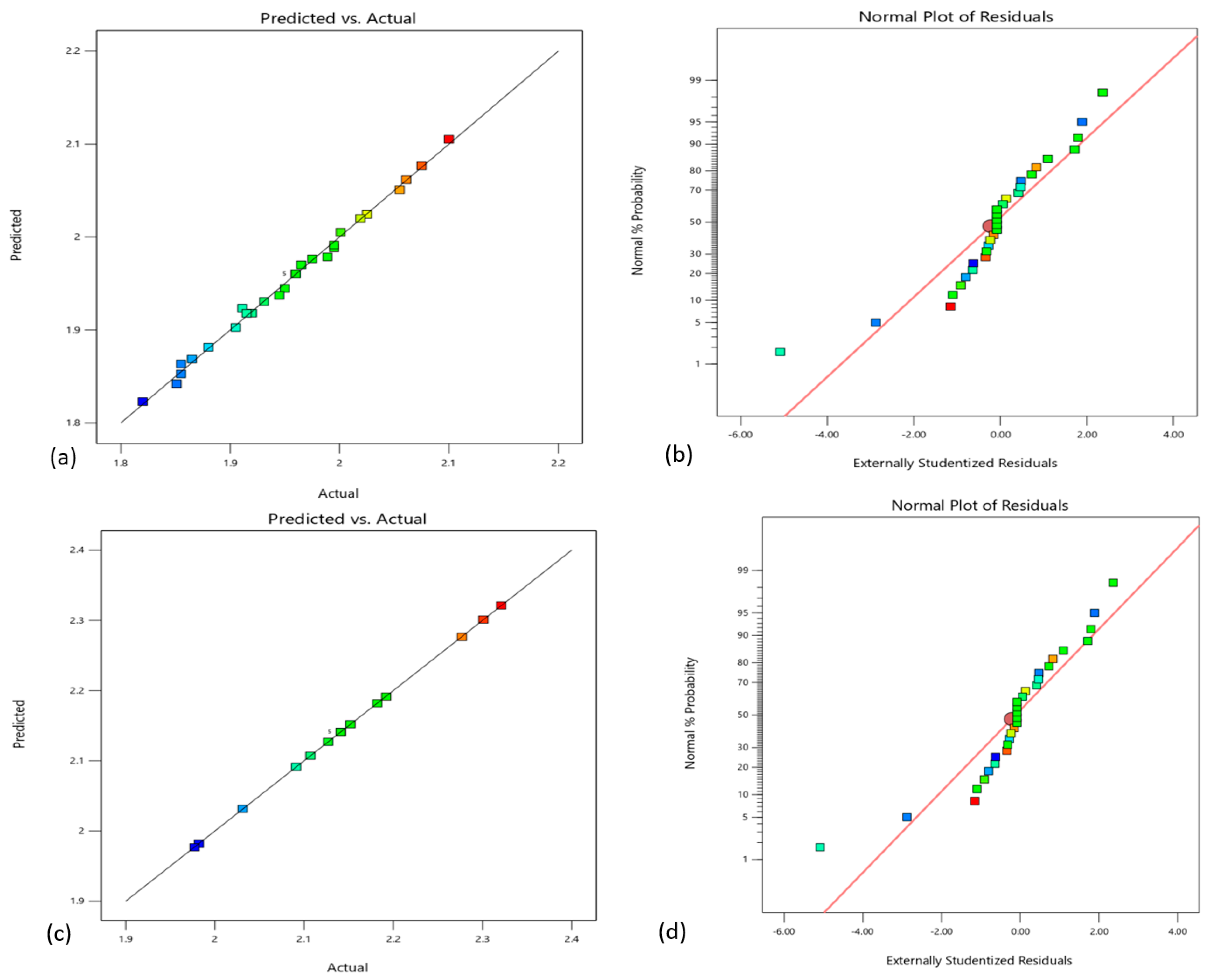
3.1.3. Actual vs. Predicted Investigative Plots for the Responses

The model plots the FWL safety coefficient’s observed vs. expected responses in Figure 3c. The graphic shows the accurate prediction and use of the FWL safety coefficient in the railway embankment slope response model. The datapoints align well with the line of best fit, indicating good agreement between actual and predicted outcomes [41]. Figure 3d depicts a randomly and sparsely scattered residual plot for the FWL safety coefficient response model, showing that errors are not correlated and have equal discrepancies. The normal residual plot is appropriate because most responses cluster around the line of fit, validating the accuracy and reliability of the generated model (Figure 3). Strength lines represent lines of best fit, while blue, green, and red dots denote the level of agreement of predicted values corresponding to low, medium, and high values of the factor of safety, respectively.

3.1.4. FWL and RWL Stability Factor Response

Three-dimensional and perturbation response graphs from the BBD-RSM show how input parameters affect output responses. The charts show how input factors affect output. Each model shows input parameters on the Y and X axes and the output (safety factor) on the Z. Figure 4 shows the interactions among FWL parameters, (a) c vs. H, (b) ϕ vs. H, (c) ρ_s vs. H, (d) ϕ vs. c, (e) ρ_s vs. c, and (f) ρ_s vs. ϕ. The a–f signified how the combined variables influenced the factor of safety. It can be seen from the plots that factor of safety (FS) increases with increase in ϕ and c, and decreases with increase in ρ_s and H. The model’s 3D contours for AC, BC, AD, and CD are relatively flat, suggesting little interaction between these factors. This shows that these two elements’ magnitudes affect the response behavior less. The vivid blue area of the plot denotes a region with minimal influence on the factor of safety, while the reddish-orange area indicates a region of optimal influence. Also the contour plots show response values in blue, green, and red classes. The colors indicate low, moderate, and very ideal interaction [41].

Figure 5 depicts the interactions among RWL parameters in 3D for (a) ϕ vs. c, (b) ρ_s vs. c, and (c) ρ_s vs. ϕ, while (d) ϕ vs. c, (e) ρ_s vs. c, and (f) ρ_s vs. ϕ represents the 2D. The a–f signified how the combined variables influenced the factor of safety for both 3D and 2D surfaces. From the 2D plots, it is shown that the FS is maximized when ϕ = 37.4 °C, c = 15.4 Kpa, and ρ_s = 1710 kg/m³. Both 2D and 3D response surface diagnostic plots show sloping flat and color margin contour profiles, indicating a strong joint interaction between independent variables [53]. The charts show that each of these factors significantly affects safety. The safety factor increases as unit weight decreases by 10–20%. An increase in the input variables cohesion and internal friction angle, is positively correlated with the stability factor. The BBD-RSM perturbation analysis shows an inverse relationship between unit weight and the two remaining input variables (cohesion and internal friction angle). The flatness of the 3D surface suggests that changes in one parameter and its effects on the factor of safety are relatively constant across the range of values of the second parameter, and vice versa, while the overall effects of these parameters are significant.

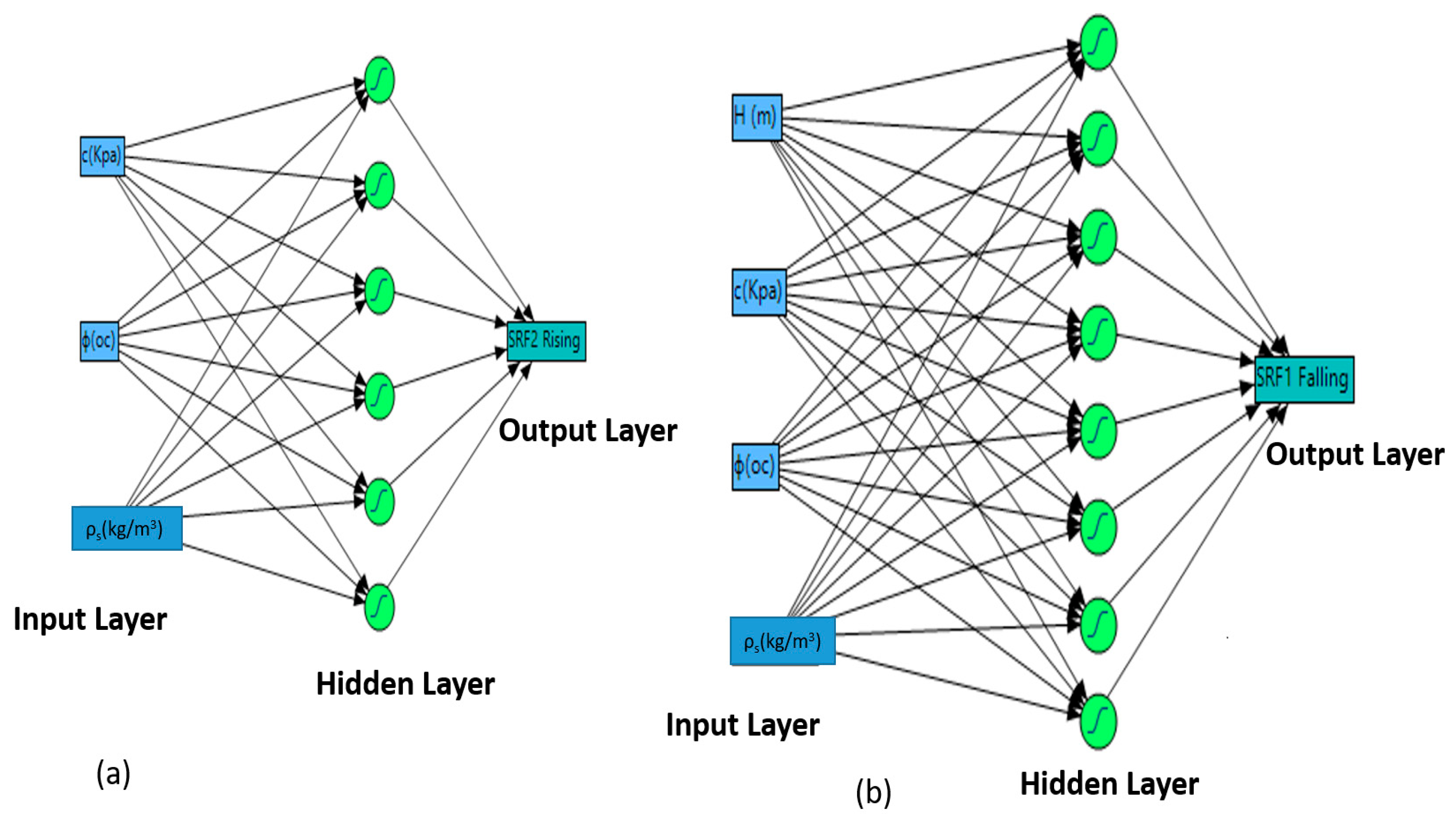
3.2. The Modeling and Optimization of Artificial Neural Networks

Building an artificial neural network required identifying model ambiguity and choosing a network design to reduce input integration mistakes and improve efficiency [53]. A neural network (ANN) was used to assess hydromechanical parameter efficacy [54,55]. The RWL stability coefficient input parameters are cohesion, internal friction angle, and unit weight (

Table 4. ANN model optimization standards.

Parameters/Responses	Lowest and Highest Limits	Goal	Weight	Importance
Friction angle	30.6–37.4	In range	1	3
Cohesion	12.6–15.4	In range	1	3
Unit weight	1710–2090	In range	1	3
Water level	15.3–18.7	In range	1	3
SRF rising	–2.3(2)	Maximize	1	3
SRF falling	–2.1	Maximize	1	3

). The FWL stability coefficient input factors are cohesion, internal friction angle, water level, and unit weight. Due to differential initial conditions, the output factors, RWL stability coefficient, and FWL stability coefficient were examined separately. A “feed-forward back-propagation” network design was used to handle the modeling system’s complexity and parameter selection [56]. The FWL network had a 4-8-1-layer pattern with eight hidden layer neurons to connect the input and output layers. Table 4 shows the statistical model values used for all neuron architectural standards (Figure 6).

The statistical analysis showed a strong positive correlation between the actual and predicted responses of the artificial neural network (ANN) model at a 95% confidence interval, indicating high agreement. The RWL had R² values of 0.99(99), 0.97(70), and 0.99(91), and FWL had R² values of 0.99(97), 0.97(71), and 0.99(56) as training, testing, validation, respectively (

Table 5. ANN optimized design for the prediction of stability coefficient.

S/N	Designs	RWL			FWL
		R2	RMSE	MAD	R2	RMSE	MAD
1	(3)	0.98(30)	0.00(75)	0.00(62)	0.99(86)	0.00(28)	0.00(21)
2	(4)	0.99(88)	0.00(12)	0.00(18)	0.99(93)	0.00(20)	0.00(16)
3	(5)	0.99(91)	0.00(18)	0.00(14)	0.99(05)	0.00(72)	0.00(56)
4	(6)	0.99(99)	1.17 × 10−15	8.88 × 10−16	0.99(96)	0.00(14)	0.00(11)
5	(7)	0.99(91)	0.00(17)	0.00(14)	0.99(67)	0.00(43)	0.00(34)
6	(8)	0.99(91)	0.00(17)	0.00(13)	0.99(97)	0.00(14)	0.00(11)
7	(9)	0.99(91)	0.00(17)	0.00(13)	0.99(99)	0.00(14)	0.00(11)
8	(10)	0.99(91)	0.00(17)	0.00(13)	0.99(69)	0.00(41)	0.00(34)

). The output of each hidden layer neuron was used to determine the optimal artificial neural network (ANN) model’s predicted results. In Equations (10) and (11), the optimized ANN-based model-predicted responses were determined with the use of output from individual neuron in the hidden layer, by adding the individual neuron and its weight.

$$H_i=\mathit{tan}h\left(0.5\left({\displaystyle \sum }_{m=1}^{N_i}\left(W_{i,m}{X}_m\right)+b_i\right)\right)$$

(10)

$$Y_{ANN}={\displaystyle \sum }_{i=1}^{N_h}\left(W_{2,i}{H}_i\right)+b_h$$

(11)

where, $H_i$ represents the hidden layer output, $X_m$ represents the corresponding input variable value, and b_h and bi are the biases hidden layers and the input, respectively [57]. Sensitivity analysis was carried out based on the relative importance of individual operating variable (input parameter) on the ANN model output (Y).

Sensitivity was evaluated on the proposed approach [44], Equation (12), which uses the neural network weight indices (i.e., layer and input weights). The fundamental principle is based on the use of the connection weights predicted by the model and then computed using Equation (12) as follows:

$$I_j=\frac{{{\displaystyle \sum }}_{m=i}^{m=N_h}\left\{\left(\frac{⎡W_{jm}^{jh}⎤}{{{\displaystyle \sum }}_{k=1}^{N_i}⎡W_{jm}^{jh}⎤}\right)\times \left|W_{mn}^{ho}\right|\right\}}{{{\displaystyle \sum }}_{k=1}^{k=N_i}\left\{{{\displaystyle \sum }}_{m=1}^{m=N_h}\left(\frac{⎡W_{km}^{jh}⎤}{{{\displaystyle \sum }}_{k=1}^{N_i}⎡W_{km}^{jh}⎤}\right)\times ⎡W_{mn}^{ho}⎤\right\}}\times 100\%$$

(12)

where $I_j$ denotes the j^th variable relative importance (%) on the ANN-based model output, N_i, N_h are the input layer and hidden neurons, respectively, and W represents the ANN model connection weight. The matrices o, i, and h stand for the output, input, and hidden layers, respectively, while n, k, and m, are the neuron numbers at the output, input, and hidden layers, respectively (Figure 7 and Figure 8).

In the RWL scenario, cohesion, internal friction angle, and unit weight were identified as significant factors in determining the stability factor. In the FWL scenario, cohesion, internal friction angle, water level, and unit weight were key. Notably, the internal friction angle had the most substantial impact, accounting for 62.8% for RWL and 53.1% for FWL. Following this, unit weight contributed 22.4% for RWL and 5.2% for FWL, while cohesion accounted for 17.8% for RWL and 32.6% for FWL and water level accounted for 10.1% for FWL. This analysis underscores the crucial role of the internal friction angle in driving stability factors.

3.3. Performance Comparison between BBD-RSM and ANN Models

Numerous researchers have shown that design within response surface methodology (BBD-RSM) and artificial neural network (ANN) modeling for sensitivity analysis is effective [41,44,58]. This work shows forecast stability coefficients with varying water levels using BBD-RSM and ANN. To assess their predictions’ accuracy, the study compared predicted and actual data and calculated absolute relative error (ARE).

Figure 9 shows the comparison between the data from the ANN and BBD-RSM models and the actual data to determine model accuracy. Scatter plots comparing each value to the number of runs showed that model-predicted values matched actual values. This comparison study found that the BBD-RSM model aligned data better than the ANN model. Thus, the BBD-RSM model slightly outperformed the ANN model in data representation.

The study also found that BBD-RSM models predicted responses marginally better. However, both the BBD-RSM and ANN models accurately predicted numerical findings and validated them across diverse data combinations utilized to investigate water level changes, whether rising or falling. The appropriateness of the BBD-RSM and ANN-based models was further examined using R², MRE, and RMSE (

Table 6. Statistical performance rating index.

Responses	R2		MRE		RMSE
	RSM	ANN	RSM	ANN	RSM	ANN
RWL	0.99(99)	0.99(99)	0.01(04)	0.17(84)	0.00(03)	0.00(84)
FWL	0.99(25)	0.99(97)	0.23(90)	0.21(15)	0.00(05)	0.00(54)

). The significant relationship between these indicators shows the models can imitate real-world outcomes. However, the time lag between surface water and groundwater should be further investigated to validate the results of this study.

4. Conclusions

This study introduced a new global static sensitivity assessment and optimization method. The Nanhu railway embankment in Hunan Province, China, was used to test this method’s efficacy and accuracy. This study was validated using field data from the year 2020, specifically focusing on the failure that occurred in the section of the K1430 + 110 of the Beijing–Guangzhou railway embankment. However, the authors are currently investigating the long-term coupled impacts of water level fluctuations and environmental factors within the watershed. The results of this study’s findings on the hydromechanical properties of the railway slope between two lakes and its process optimization possibilities are as follows:

• The investigation showed a substantial link between the embankment slope seepage line and lakes water level fluctuations. The Plackett–Burman design was used to independently study the parameters that significantly affect the railway slope’s total static stability factor under rising and falling water levels. Key parameters, such as angle of internal friction (ϕ), soil density (ρ_s), and cohesion (c), significantly impact the slope stability during a rise in water level. However, k_s, H, u, v, and E were less significant. During falling water levels, ϕ, c, H, and ρ_s were more important but in a different sequence.
• The BBD-RSM and ANN studies used 3D surface and profiler diagrams to find factor–response relationships. These diagrams accurately predicted the components needed to fulfil goals. The predicted results were supported by ANOVA models. The study found some notable second-order interactions. RWL interactions were c x ρ_s, ϕ x ρ_s, and ρ_s², and the FWL interactions were H x c and c x ρ_s. We also found that RWL was more consistent at higher unit weights and FWL was more stable at lower unit weights. RWL’s finest factor combinations are (14.11, 37.4, and 1711.9), and FWL’s are (14.175, 37.4, 15.529, and 1713.24)
• The research found that BBD-RSM and ANN were effective for evaluating RWL and FWL stability coefficients. All input variables affected the coefficients, but angle of internal friction had the greatest impact, followed by soil density and then cohesion for the RWL. The angle of internal friction had the greatest impact on FWL, followed by cohesion, water level, and soil density. Compared to ANN-based models, RSM-based models performed slightly better during RWL, with comparable R² values but fewer prediction errors (RMSE and MRE). Compared to RSM-based models, the RSM model produced R² values of 0.99(99) and 0.99 with MREs of 0.01 and 0.24 under both RWL and FWL conditions, respectively. However, for ANN, respectively, they produced R² values of 0.99(99) and 0.99(98), with MRE values of 0.02 and 0.21, indicating that ANN-based models performed slightly better during FWL, with higher R² values and reduced prediction errors (MRE). Coupled analysis with RSM and ANN models improved accuracy, efficiency, iteration needs, trial durations, and cost-effectiveness for both experimental and numerical processes.

References

1. Briggs, K.; Loveridge, F.; Glendinning, S. Failures in transport infrastructure embankments. Eng. Geol. 2017, 219, 107–117. [Google Scholar] [CrossRef]
2. Reale, C.; Gavin, K.; Martinovic, K. Analysing the effect of rainfall on railway embankments using fragility curves. In Proceedings of the Transport Research Arena 2018: A Digital Era for Transport, Vienna, Austria, 16–19 April 2018. [Google Scholar]
3. Linrong, X.; Usman, A.B.; Bello, A.-A.D.; Yongwei, L. Rainfall-induced transportation embankment failure: A review. Open Geosci. 2023, 15, 20220558. [Google Scholar] [CrossRef]
4. Kite, D.; Siino, G.; Audley, M. Detecting Embankment Instability Using Measurable Track Geometry Data. Infrastructures 2020, 5, 29. [Google Scholar] [CrossRef]
5. Dai, Z.; Guo, J.; Yu, F.; Zhou, Z.; Li, J.; Chen, S. Long-term uplift of high-speed railway subgrade caused by swelling effect of red-bed mudstone: Case study in Southwest China. Bull. Eng. Geol. Environ. 2021, 80, 4855–4869. [Google Scholar] [CrossRef]
6. Sheng, M.-H.; Ai, X.-Y.; Huang, B.-C.; Zhu, M.-K.; Liu, Z.-Y.; Ai, Y.-W. Effects of biochar additions on the mechanical stability of soil aggregates and their role in the dynamic renewal of aggregates in slope ecological restoration. Sci. Total Environ. 2023, 898, 165478. [Google Scholar] [CrossRef]
7. Shuaibu, A.; Muhammad, M.M.; Bello, A.-A.D.; Sulaiman, K.; Kalin, R.M. Flood Estimation and Control in a Micro-Watershed Using GIS-Based Integrated Approach. Water 2023, 15, 4201. [Google Scholar] [CrossRef]
8. Wang, L.; Wu, C.; Gu, X.; Liu, H.; Mei, G.; Zhang, W. Probabilistic stability analysis of earth dam slope under transient seepage using multivariate adaptive regression splines. Bull. Eng. Geol. Environ. 2020, 79, 2763–2775. [Google Scholar] [CrossRef]
9. Yao, J.; Chen, Y.; Guan, X.; Zhao, Y.; Chen, J.; Mao, W. Recent climate and hydrological changes in a mountain–basin system in Xinjiang, China. Earth-Sci. Rev. 2022, 226, 103957. [Google Scholar] [CrossRef]
10. Isidoro, J.M.; Martins, R.; Carvalho, R.F.; de Lima, J.L. A high-frequency low-cost technique for measuring small-scale water level fluctuations using computer vision. Measurement 2021, 180, 109477. [Google Scholar] [CrossRef]
11. Fan, Z.; Zheng, H.; Liu, K.; Chen, C.; Yang, F. Investigation of the shear band evolution in soil-rock mixture using the assumed enhanced strain method with the meshes of improved numerical manifold method. Eng. Anal. Bound. Elem. 2022, 144, 530–538. [Google Scholar] [CrossRef]
12. Yi, S.; Liu, J. Field investigation of steel pipe pile under lateral loading in extensively soft soil. Front. Mater. 2022, 9, 971485. [Google Scholar] [CrossRef]
13. Xie, Y.; Feng, S.-J.; Xiong, Y.-L.; Zhang, L.-L.; Ye, G.-L. Coupled hydraulic-mechanical-air simulation of unsaturated railway embankment under rainfall and dynamic train load. Transp. Geotech. 2021, 27, 100463. [Google Scholar] [CrossRef]
14. Wan, X.; Ding, J.; Hong, Z.; Huang, C.; Shang, S.; Ding, C. Dynamic Response of a Low Embankment Subjected to Traffic Loads on the Yangtze River Floodplain, China. Int. J. Geomech. 2022, 22, 04022065. [Google Scholar] [CrossRef]
15. Wang, R.; Hu, Z.; Ma, J.; Ren, X.; Li, F.; Zhang, F. Dynamic response and long-term settlement of a compacted loess embankment under moving train loading. KSCE J. Civ. Eng. 2021, 25, 4075–4087. [Google Scholar] [CrossRef]
16. Sushma, M.; Bhushan, J.S.; Madhav, M.R. Assessment of Stability of Embankments on Soft Ground Using Matsuo Chart and SLOPE/W. In Best Practices in Geotechnical and Pavement Engineering; Springer: Berlin/Heidelberg, Germany, 2023; pp. 71–78. [Google Scholar]
17. Zhou, C.; Shen, Z.; Xu, L.; Sun, Y.; Zhang, W.; Zhang, H.; Peng, J. Global Sensitivity Analysis Method for Embankment Dam Slope Stability Considering Seepage–Stress Coupling under Changing Reservoir Water Levels. Mathematics 2023, 11, 2836. [Google Scholar] [CrossRef]
18. Ni, J.; Leung, A.; Ng, C.; Shao, W. Modelling hydro-mechanical reinforcements of plants to slope stability. Comput. Geotech. 2018, 95, 99–109. [Google Scholar] [CrossRef]
19. Boldrin, D.; Leung, A.K.; Bengough, A.G. Hydro-mechanical reinforcement of contrasting woody species: A full-scale investigation of a field slope. Géotechnique 2021, 71, 970–984. [Google Scholar] [CrossRef]
20. Mohsan, M.; Vossepoel, F.C.; Vardon, P.J. On the use of different data assimilation schemes in a fully coupled hydro-mechanical slope stability analysis. Georisk Assess. Manag. Risk Eng. Syst. Geohazards 2023, 18, 121–137. [Google Scholar] [CrossRef]
21. Hou, D.; Zhou, Y.; Zheng, X. Seepage and stability analysis of fissured expansive soil slope under rainfall. Indian Geotech. J. 2023, 53, 180–195. [Google Scholar] [CrossRef]
22. Shuaibu, A.; Hounkpè, J.; Bossa, Y.A.; Kalin, R.M. Flood Risk Assessment and Mapping in the Hadejia River Basin, Nigeria, Using Hydro-Geomorphic Approach and Multi-Criterion Decision-Making Method. Water 2022, 14, 3709. [Google Scholar] [CrossRef]
23. Shuaibu, A.; Kalin, R.M.; Phoenix, V.; Banda, L.C.; Lawal, I.M. Hydrogeochemistry and Water Quality Index for Groundwater Sustainability in the Komadugu-Yobe Basin, Sahel Region. Water 2024, 16, 601. [Google Scholar] [CrossRef]
24. Wang, T.; Luo, Q.; Li, Z.; Zhang, W.; Chen, W.; Wang, L. System safety assessment with efficient probabilistic stability analysis of engineered slopes along a new rail line. Bull. Eng. Geol. Environ. 2022, 81, 68. [Google Scholar] [CrossRef]
25. Moldovan, D.-V.; Nagy, A.-C.; Muntean, L.-E.; Ciotlaus, M. Study on the stability of a road fill embankment. Procedia Eng. 2017, 181, 60–67. [Google Scholar] [CrossRef]
26. Zewdu, A. Modeling the slope of embankment dam during static and dynamic stability analysis: A case study of Koga dam, Ethiopia. Model. Earth Syst. Environ. 2020, 6, 1963–1979. [Google Scholar] [CrossRef]
27. Gao, X.; Liu, H.; Zhang, W.; Wang, W.; Wang, Z. Influences of reservoir water level drawdown on slope stability and reliability analysis. Georisk Assess. Manag. Risk Eng. Syst. Geohazards 2019, 13, 145–153. [Google Scholar] [CrossRef]
28. Chen, J.; Zhou, Y. Dynamic responses of subgrade under double-line high-speed railway. Soil Dyn. Earthq. Eng. 2018, 110, 1–12. [Google Scholar] [CrossRef]
29. Ahmad, F.; Tang, X.-W.; Qiu, J.-N.; Wróblewski, P.; Ahmad, M.; Jamil, I. Prediction of slope stability using Tree Augmented Naive-Bayes classifier: Modeling and performance evaluation. Math. Biosci. Eng. 2022, 19, 4526–4546. [Google Scholar] [CrossRef] [PubMed]
30. Abdalla, J.A.; Attom, M.F.; Hawileh, R. Prediction of minimum factor of safety against slope failure in clayey soils using artificial neural network. Environ. Earth Sci. 2015, 73, 5463–5477. [Google Scholar] [CrossRef]
31. Tao, G.L.; Yao, Z.S.; Tan, B.Z.; Gao, C.C.; Yao, Y.W. Application of support vector machine for prediction of slope stability coefficient considering the influence of rainfall and water level. Appl. Mech. Mater. 2016, 851, 840–845. [Google Scholar] [CrossRef]
32. Zhang, H.; Nguyen, H.; Bui, X.-N.; Pradhan, B.; Asteris, P.G.; Costache, R.; Aryal, J. A generalized artificial intelligence model for estimating the friction angle of clays in evaluating slope stability using a deep neural network and Harris Hawks optimization algorithm. Eng. Comput. 2021, 38, 3901–3914. [Google Scholar] [CrossRef]
33. Hu, L.; Takahashi, A.; Kasama, K. Effect of spatial variability on stability and failure mechanisms of 3D slope using random limit equilibrium method. Soils Found. 2022, 62, 101225. [Google Scholar] [CrossRef]
34. Zhang, W.; Shen, Z.; Ren, J.; Bian, J.; Xu, L.; Chen, G. Multifield Coupling Numerical Simulation of the Seepage and Stability of Embankment Dams on Deep Overburden Layers. Arab. J. Sci. Eng. 2022, 47, 7293–7308. [Google Scholar] [CrossRef]
35. Zhou, T.; Zhang, L.; Cheng, J.; Wang, J.; Zhang, X.; Li, M. Assessing the rainfall infiltration on FOS via a new NSRM for a case study at high rock slope stability. Sci. Rep. 2022, 12, 11917. [Google Scholar] [CrossRef] [PubMed]
36. Yu, S.; Ren, X.; Zhang, J.; Wang, H.; Wang, J.; Zhu, W. Seepage, deformation, and stability analysis of sandy and clay slopes with different permeability anisotropy characteristics affected by reservoir water level fluctuations. Water 2020, 12, 201. [Google Scholar] [CrossRef]
37. Mojtahedi, S.F.F.; Tabatabaee, S.; Ghoroqi, M.; Tehrani, M.S.; Gordan, B.; Ghoroqi, M. A novel probabilistic simulation approach for forecasting the safety factor of slopes: A case study. Eng. Comput. 2019, 35, 637–646. [Google Scholar] [CrossRef]
38. Ian, V.-K.; Tse, R.; Tang, S.-K.; Pau, G. Bridging the Gap: Enhancing Storm Surge Prediction and Decision Support with Bidirectional Attention-Based LSTM. Atmosphere 2023, 14, 1082. [Google Scholar] [CrossRef]
39. Gordan, B.; Armaghani, D.J.; Hajihassani, M.; Monjezi, M. Prediction of seismic slope stability through combination of particle swarm optimization and neural network. Eng. Comput. 2016, 32, 85–97. [Google Scholar] [CrossRef]
40. Dragović, S. Artificial neural network modeling in environmental radioactivity studies—A review. Sci. Total Environ. 2022, 847, 157526. [Google Scholar] [CrossRef] [PubMed]
41. Yaro, N.S.A.; Sutanto, M.H.; Habib, N.Z.; Napiah, M.; Usman, A.; Muhammad, A. Comparison of Response Surface Methodology and Artificial Neural Network approach in predicting the performance and properties of palm oil clinker fine modified asphalt mixtures. Constr. Build. Mater. 2022, 324, 126618. [Google Scholar] [CrossRef]
42. Lafifi, B.; Rouaiguia, A.; Soltani, E.A. A Novel Method for Optimizing Parameters influencing the Bearing Capacity of Geosynthetic Reinforced Sand Using RSM, ANN, and Multi-objective Genetic Algorithm. Stud. Geotech. Mech. 2023, 45, 174–196. [Google Scholar] [CrossRef]
43. Plackett, R.L.; Burman, J.P. The design of optimum multifactorial experiments. Biometrika 1946, 33, 305–325. [Google Scholar] [CrossRef]
44. De Luna, M.D.G.; Sablas, M.M.; Hung, C.-M.; Chen, C.-W.; Garcia-Segura, S.; Dong, C.-D. Modeling and optimization of imidacloprid degradation by catalytic percarbonate oxidation using artificial neural network and Box-Behnken experimental design. Chemosphere 2020, 251, 126254. [Google Scholar] [CrossRef]
45. Aziz, K.; Mamouni, R.; Azrrar, A.; Kjidaa, B.; Saffaj, N.; Aziz, F. Enhanced biosorption of bisphenol A from wastewater using hydroxyapatite elaborated from fish scales and camel bone meal: A RSM@ BBD optimization approach. Ceram. Int. 2022, 48, 15811–15823. [Google Scholar] [CrossRef]
46. Buscema, M. Back propagation neural networks. Subst. Use Misuse 1998, 33, 233–270. [Google Scholar] [CrossRef]
47. Yang, C.; Liu, K.; Yang, S.; Zhu, W.; Tong, L.; Shi, J.; Wang, Y. Prediction of metformin adsorption on subsurface sediments based on quantitative experiment and artificial neural network modeling. Sci. Total Environ. 2023, 899, 165666. [Google Scholar] [CrossRef]
48. Li, S.; Li, Y.; Xu, L. Deformation Pattern and Failure Mechanism of Railway Embankment Caused by Lake Water Fluctuation Using Earth Observation and On-Site Monitoring Techniques. Water 2023, 15, 4284. [Google Scholar] [CrossRef]
49. Igwe, O.; Chukwu, C. Slope stability analysis of mine waste dumps at a mine site in Southeastern Nigeria. Bull. Eng. Geol. Environ. 2019, 78, 2503–2517. [Google Scholar] [CrossRef]
50. Rahimi, A.; Rahardjo, H.; Leong, E.-C. Effect of antecedent rainfall patterns on rainfall-induced slope failure. J. Geotech. Geoenvironmental Eng. 2011, 137, 483–491. [Google Scholar] [CrossRef]
51. Rahardjo, H.; Nistor, M.-M.; Gofar, N.; Satyanaga, A.; Xiaosheng, Q.; Yee, S.I.C. Spatial distribution, variation and trend of five-day antecedent rainfall in Singapore. Georisk Assess. Manag. Risk Eng. Syst. Geohazards 2020, 14, 177–191. [Google Scholar] [CrossRef]
52. Kim, S.W.; Chun, K.W.; Kim, M.; Catani, F.; Choi, B.; Seo, J.I. Effect of antecedent rainfall conditions and their variations on shallow landslide-triggering rainfall thresholds in South Korea. Landslides 2021, 18, 569–582. [Google Scholar] [CrossRef]
53. Isiyaka, H.A.; Jumbri, K.; Sambudi, N.S.; Zango, Z.U.; Abdullah, N.A.F.; Saad, B.; Mustapha, A. Adsorption of dicamba and MCPA onto MIL-53 (Al) metal–organic framework: Response surface methodology and artificial neural network model studies. RSC Adv. 2020, 10, 43213–43224. [Google Scholar] [CrossRef] [PubMed]
54. Foong, L.K.; Moayedi, H. Slope stability evaluation using neural network optimized by equilibrium optimization and vortex search algorithm. Eng. Comput. 2021, 38, 1269–1283. [Google Scholar] [CrossRef]
55. Bharati, A.K.; Ray, A.; Khandelwal, M.; Rai, R.; Jaiswal, A. Stability evaluation of dump slope using artificial neural network and multiple regression. Eng. Comput. 2022, 38 (Suppl. S3), 1835–1843. [Google Scholar] [CrossRef]
56. Gelisli, K.; Kaya, T.; Babacan, A.E. Assessing the factor of safety using an artificial neural network: Case studies on landslides in Giresun, Turkey. Environ. Earth Sci. 2015, 73, 8639–8646. [Google Scholar] [CrossRef]
57. Genuino, D.A.D.; Bataller, B.G.; Capareda, S.C.; de Luna, M.D.G. Application of artificial neural network in the modeling and optimization of humic acid extraction from municipal solid waste biochar. J. Environ. Chem. Eng. 2017, 5, 4101–4107. [Google Scholar] [CrossRef]
58. Betiku, E.; Taiwo, A.E. Modeling and optimization of bioethanol production from breadfruit starch hydrolyzate vis-à-vis response surface methodology and artificial neural network. Renew. Energy 2015, 74, 87–94. [Google Scholar] [CrossRef]
Figure 1. Map slope stability analysis studies under water level using VOSviewer.
Applsci 14 03402 g001
Figure 2. (a) Nanhu Embankment location map in Hunan province, China, (b) administrative boundaries map of Yueyang Study area location, and (c) location and cross-section of the embankment.
Applsci 14 03402 g002
Figure 3. Investigative plots for (a,b) RWL and (c,d) FWL model suitability.
Applsci 14 03402 g003
Figure 4. Three-dimensional response surface plots displaying the influence of all parameters on FWL coefficient.
Applsci 14 03402 g004
Figure 5. Two-dimensional and three-dimensional response surface plots displaying the influence of all parameters on RWL coefficient.
Applsci 14 03402 g005
Figure 6. ANN neuron design for the (a) RWL and (b) FWL response.
Applsci 14 03402 g006
Figure 7. ANN model RWL response graph of predicted and actual values for (a) training, (b) validation, (c) testing, and (d) optimization profiler.
Applsci 14 03402 g007
Figure 8. ANN model FWL response graph of predicted and actual values for (a) training, (b) validation, (c) testing, and (d) optimization profiler.
Applsci 14 03402 g008
Figure 9. Comparative evaluation between ANN and BBD-RSM models predictions values with the actual values for (a) RWL and (b) FWL response.
Applsci 14 03402 g009