
Multilevel Distributed Linear State Estimation Integrated with Transmission Network Topology Processing


Real-Time Power and Intelligent Systems Laboratory, Holcombe Department of Electrical and Computer Engineering, Clemson University, Clemson, SC 29634, USA
*
Author to whom correspondence should be addressed.
Appl. Sci. 2024, 14(8), 3422; https://doi.org/10.3390/app14083422
Submission received: 8 March 2024
/
Revised: 4 April 2024
/
Accepted: 16 April 2024
/
Published: 18 April 2024
(This article belongs to the Special Issue New Insights into Power System Resilience)
Abstract
:State estimation (SE) is an important energy management system application for power system operations. Linear state estimation (LSE) is a variant of SE based on linear relationships between state variables and measurements. LSE estimates system state variables, including bus voltage magnitudes and angles in an electric power transmission network, using a network model derived from the topology processor and measurements. Phasor measurement units (PMUs) enable the implementation of LSE by providing synchronized high-speed measurements. However, as the size of the power system increases, the computational overhead of the state-of-the-art (SOTA) LSE grows exponentially, where the practical implementation of LSE is challenged. This paper presents a distributed linear state estimation (D-LSE) at the substation and area levels using a hierarchical transmission network topology processor (H-TNTP). The proposed substation-level and area-level D-LSE can efficiently and accurately estimate system state variables at the PMU rate, thus enhancing the estimation reliability and efficiency of modern power systems. Network-level LSE has been integrated with H-TNTP based on PMU measurements, thus enhancing the SOTA LSE and providing redundancy to substation-level and area-level D-LSE. The implementations of D-LSE and enhanced LSE have been investigated for two benchmark power systems, a modified two-area four-machine power system and the IEEE 68 bus power system, on a real-time digital simulator. The typical results indicate that the proposed multilevel D-LSE is efficient, resilient, and robust for topology changes, bad data, and noisy measurements compared to the SOTA LSE.
1. Introduction
Traditional state estimation was introduced to the power system by Fred Schweppe in 1970 in [1,2,3] to process available imperfect information (noise, bad data, or false data) [4,5] and produces the best possible estimates for the state variables in consideration. However, the traditional static state estimation is inefficient in estimating state variables in modern power systems. The modern bulk power system is increasingly integrated with inverter-based resources such as solar photovoltaic and wind. The electric power system distribution system is becoming more active with the effect of distributed energy sources, microgrid operations, electric vehicle inclusion, spot loads, and demand response programs, which aggregate at substations, thereby influencing the transmission network. Furthermore, the modern world is moving towards an integrated energy system, where other critical energy infrastructures, including natural gas and transportation, are corporately operated with the electrical power system for improved energy efficiency [6], and the modern power system is influenced by factors outside the energy control centers’ operation. State estimation is foundational for applications such as security-constrained optimal power flow [7], economic dispatch [8], contingency analysis [9], and security assessment [10]. Thus, an efficient approach for state estimation is favorable over the traditional state estimation in the modern power system.
State-of-the-art (SOTA) linear state estimation (LSE) has improved the estimation capabilities [11], where efficient measurements are used to establish a linear relationship with the state variables. LSE can accurately estimate bus node voltage phasors utilizing measurements such as available the noisy voltage phasor and current phasor measurements. LSE can be implemented solely based on the phasor measurement units (PMUs) [12] and the network model. The network model of the SOTA LSE is derived from the SOTA transmission network topology processing (TNTP) approach, which is based on the asynchronous supervisory control and data acquisition (SCADA) monitoring of relay signals (SMRS), where the reliability can be challenged [13,14] and only updates the topology from 2 s to 5 s [15]. Furthermore, the SOTA LSE is not scalable for large power systems, because computation time increases rapidly with the size of the network. The power system transmission network is a large, geographically distributed network. Thus, a distributed architecture is favorable to ensure the efficient process of the LSE with PMU measurements.
A comprehensive analysis of the state estimation has been conducted in [16], where shortcomings of the literature and existing operational state estimations have been identified, including accuracy and security. In [17], a robust hybrid state estimator was built against the non-Gaussian noise in PMU measurements; the filtration process utilized SCADA-based state estimation, which still limits the efficiency achieved by the PMU-only state estimation. Distributed state estimation architectures for multiarea power systems have been proposed in [8,18,19,20]. The different architectures utilize the least squares estimation techniques and information exchange between the control areas. Although distributed architecture improves computational efficiency, the approaches are based on traditional iterative estimation methods, where the efficiency is compromised. A semidefinite programming formulation based on distributed state estimation utilizing synchrophasor measurements was studied in [21]. Both proposed approaches in [21] involve the legacy SE and the PMU-based linear estimation, which increase the computational burden. The incorporation of linear and nonlinear models for state estimation has been investigated in [22]. The system is divided into multiple linear and nonlinear areas, which define the distributed architecture of the study. The procedure is expected to be completed based on sequential flow, where the efficiency achieved from PMU measurement-based LSE in the linear regions is compromised. PMU-based topology derivation and extended LSE implementation were studied in [23], where the test system used the breaker status as a digital input to the PMU. Digital inputs in the PMUs require additional communication network upgrades from relays or remote terminal units (RTUs) to PMUs in the substation; furthermore, the proposed approach is centralized. A phasor data-based state estimator with phase bias correction has been proposed in [24]. This work identifies PMU-available high-voltage substations for building phasor state estimators. Identifying the island topology is critical; although, using SMRS in this study limits the efficiency of the overall procedure. A two-level LSE has been proposed in [25,26,27]; the proposal investigates the power system at the substation level and network level. The shortcomings of this approach are that the only redundancy for the substation level is the network level, where the computational overhead is high in larger networks. Furthermore, the study was limited to the ring bus arrangement type (RBA) substations only. The effectiveness of the overall approach can be different based on the type of substation arrangement.
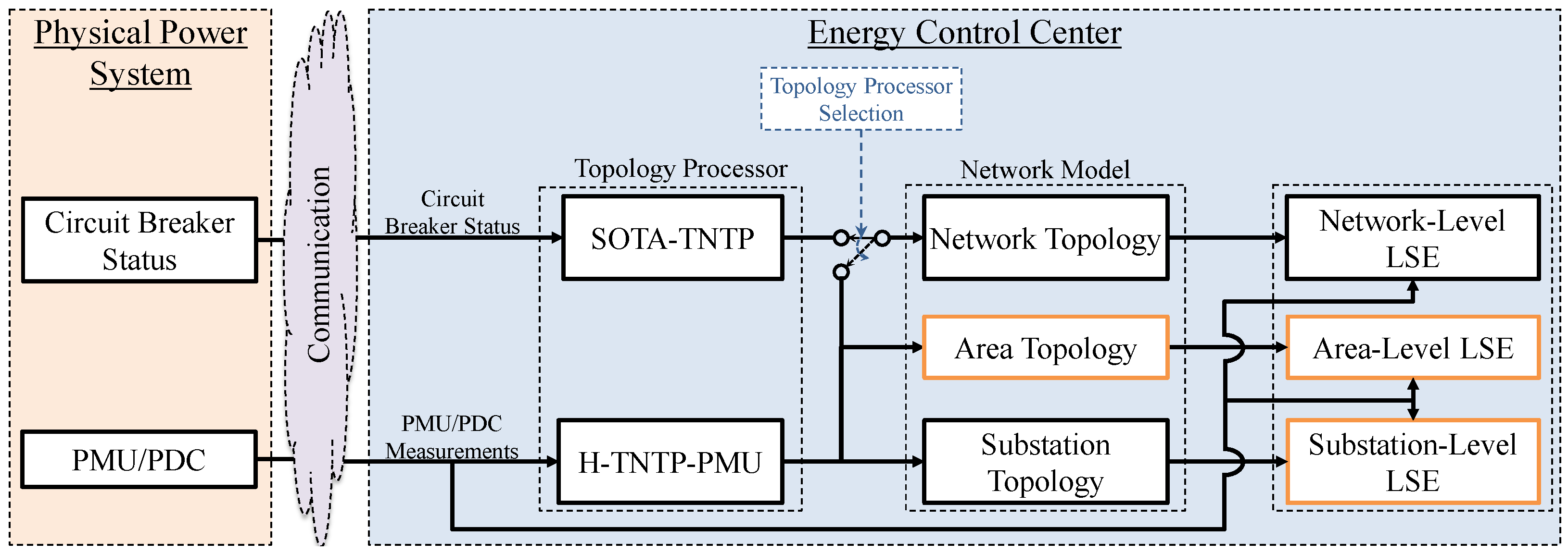
A physics-based hierarchical TNTP (H-TNTP) approach based solely on node voltages and branch currents measurements utilizing artificial intelligence algorithms was proposed in [28]. H-TNTP can be used to derive the substation area network-level topologies using current and voltage measurements, which is ideal for a distributed LSE architecture. An efficient H-TNTP can be established by incorporating the synchrophasor network (H-TNTP-PMU), which updates the transmission network topology at every PMU frame. The synchrophasor network typically delivers voltage and current phasor measurements at 30 Hz [29]. Thus, incorporating H-TNTP-PMU will enable LSE execution at every PMU measurement. This paper proposes a multilevel distributed LSE (D-LSE) architecture with substation-level and area-level estimation utilizing H-TNTP-PMU. The network level based on the SOTA LSE enhanced with the H-TNTP-PMU has been integrated as the redundancy level for the area level. The proposed approach overcomes the limitations identified in the SOTA LSE and the alternative approaches proposed by other researchers. The D-LSE incorporates the efficient and reliable H-TNTP-PMU as the topology processor, which enables the completion of the overall procedure at the PMU rate. The multilevel redundancy improves the reliability of the D-LSE. Incorporating all typical substation arrangements in the substation level ensures the applicability of the proposed D-LSE. The overview of the proposed D-LSE is shown in Figure 1.
The main contributions of this paper are the following:
- A multilevel distributed linear state estimation has been developed based on hierarchical transmission network topology processing. With the developed D-LSE, substation bus voltage phasors can be estimated at the substation level and/or area level. This caters to fast and efficient linear state estimation for large power systems.
- The traditional linear state estimation has been enhanced with H-TNTP-PMU to provide a network-level model that is updated with the same measurements used for LSE. This improves the accuracy of the traditional LSE.
- The D-LSE and enhancement to the traditional LSE have been illustrated on two benchmark test power systems. The two power systems, one small and the other medium, have been implemented on a real-time power system simulator with phasor measurement units and noisy measurements. The typical results obtained with the D-LSE and enhanced LSE demonstrate better efficiency, resilience, and robustness with respect to topology changes, bad data, and noisy measurements, respectively.
The rest of the paper is organized as follows: Section 2 presents the formulation of the proposed D-LSE architecture with the enhanced network-level estimation. An introduction to the test power system models, typical results, and the performance analysis for D-LSE with the enhanced network-level estimation are discussed in Section 3. The conclusion and future directions are provided in Section 4.
2. Methodology
The methodology section outlines the LSE formulation for the proposed D-LSE with the enhanced network-level estimation, thus providing a comprehensive clarification of its components and organization.
2.1. Linear State Estimation (LSE)
The SOTA LSE considers the entire power system to be a single entity. The formulation of the LSE described in [11] is considered for the network level as a redundancy layer for the D-LSE and to compare with substation-level and area-level estimation. The current measurement bus incidence matrix (A) presents the current flow measurement’s location in the network, where the TNTP is used to update. A is an m by b-sized matrix, where m represents the number of current measurements in the network, and b is the number of buses that have current measurements leaving the selected bus. The voltage measurement bus incidence matrix () is similar to the A, where the TNTP is used to update. It presents the relationship between a voltage measurement and its respective location in the network. It is an n by d matrix, where n represents the number of voltage measurements in the network, and d is the number of buses with voltage measurements. The series admittance matrix (y) is a diagonal matrix, where the diagonal elements are the measured admittance of the respective lines. It is k by k-sized matrix, where k represents the number of branch current measurements in the network. The shunt admittance matrix () relates the location of each current measurement to the shunt admittance of the line it measures. It is an l by g matrix, where l is the number of current measurements in the network, and g is the number of buses where the current is being originally measured. The intermediate characteristics matrix can be formed with A, , y, and using (1).
The linear relationship between measurements and the states can be formulated using (2). is referred to as the measurement residue vector.
Considering that the measurements contain noise, the covariance matrix (W) appears in the solution. Then, the solution can be found using (3).
2.2. Multilevel Distributed Linear State Estimation (D-LSE)
LSE at every PMU rate can be computationally challenging when considering the enormity of power systems. A preliminary experiment has been conducted to understand the computation overhead of the LSE procedure with respect to the network size. The computation overhead is shown in Figure 2.
Considering the overall LSE procedure discussed in Section 2.1, the number of algebraic operations and execution time are estimated for different bus-sized networks. The execution time is the computation time for matrix formation and the solution to the LSE equation in (3). The execution time is estimated by running the LSE algorithm in a dedicated node of the Clemson University Palmetto Cluster with 124 GB of memory. The computation overhead exponentially increased with the number of buses in the considered network, as shown in Figure 2. Based on the highest execution time (on the computation platform mentioned above) for executing the LSE under the PMU data rate (under 33.33 ms), the network size limit came out to 2283 buses, excluding the computation time for TNTP and communication delays. Thus, SOTA LSE is not an option for practical implementation in large power systems. Though the efficiency limitation of the SOTA LSE approach has been identified, SOTA LSE (network level) is considered a redundancy level to the area level. Furthermore, the network level will be used to compare performance with the D-LSE. The flow diagram of the procedure of the D-LSE with the enhanced network level is shown in Figure 3.
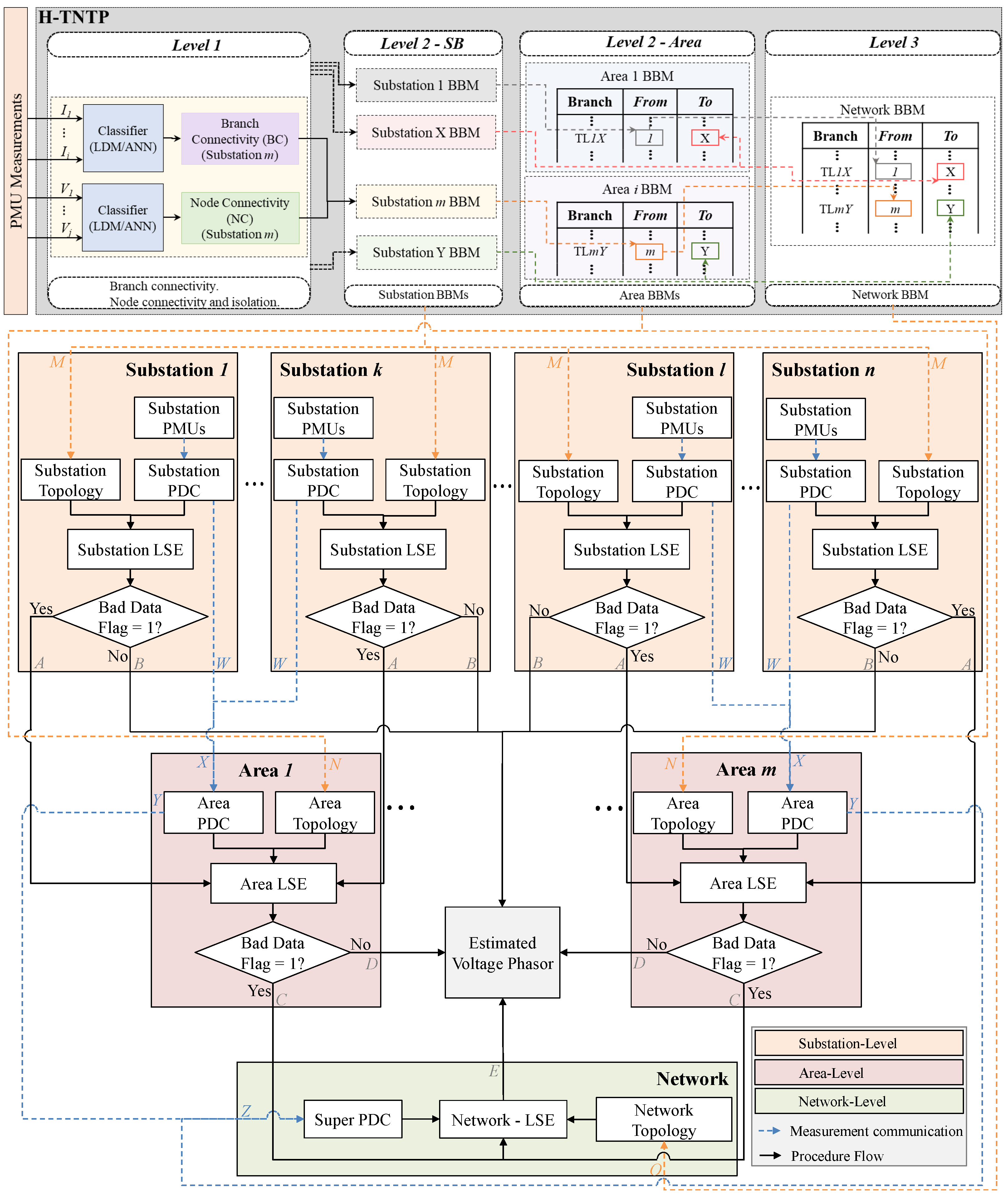
Based on the above preliminary study, it was identified that a more computationally efficient architecture for LSE is required for large multiarea power systems. Hence, the authors proposed the D-LSE architecture. The H-TNTP approach was modified to accommodate the D-LSE, as shown in Figure 3, including the area level BBM as Level 2-Area. Thus, the area level of the D-LSE will be based on Level 2-Area of the modified H-TNTP. Similarly, for the substation level of the D-LSE, H-TNTP Level 2-SB was utilized as the topology, and for the network level, Level 3 of the H-TNTP was used. The LSE can then be performed for each area and substation by keeping all PMU measurements relative to the global reference (ground in practical use). This allows substation-level or area-level D-LSE to be implemented in parallel processes.
2.3. Substation Level
A substation consists of branches, bus sections, protection equipment (relays), measurement instruments (PMUs), and switching equipment (breakers, isolators, etc.). Each piece of equipment is required for the power system’s operation and control. H-TNTP Level 2-SB shown in Figure 3 can be directly utilized to identify the substation topology. Substations are considered to be zero-impedance networks. Since Ohm’s law-based current, voltage, and impedance relationships cannot be established on a zero-impedance network, a linear relationship for currents based on the substation configuration was established following the method proposed in [25]. This is shown in Figure 3 at the substation level and elaborated in Figure 4a.
The proposed substation level LSE comprises two estimations: current state estimation and voltage state estimation. The current estimation is used for bad data detection in analog current measurements and topology errors; voltage-based bad data identification can be implemented using cellular computational networks (CCNs) [30]. When the bad data are detected at the substation level, the substation LSE raises a flag and entrusts the LSE to the area level. This is based on the assumption that bad data detection indicates a faulty PMU. Thus, the voltage phasor can also be a bad measurement. Thus, this avoids conducting simple weighted average estimation for the voltage phasor, which does not have inherent bad data detection. The is the computational time for matrix formation, is the computational time to solve breaker current estimation, and is the computational time to solve voltage estimation using a weighted average. The area-level LSE will use the bad data detection flag and conduct the area-level LSE, thereby avoiding bad data flagged substations in the area.
The current state estimation considers the circuit breaker currents as states in the LSE. Based on Kirchhoff’s Current Law (KCL), the relationship between the circuit breaker current and the injection currents in the zero impedance network can be written as (4). refers to the current injection by each node, and is the adjacent matrix that defines the relationship, which is the node connectivity matrix (NCM) of the H-TNTP Level 2. is the injection current measurement residue.
Based on the availability of the breaker current measurement, another linear relationship can be established for the breaker currents by relating the breaker current estimation to the measurements with an identity matrix, as shown in (5). refers to the breaker current measurements, I is the identity matrix, and is the breaker current measurement residue.
By combining (4) and (5), a single linear state estimation problem can be formed as (6), which again can be summarized in the form shown in (2), where the B matrix given in (7) consists of 1, 0, and −1 as elements.
Voltage state estimation is conducted at the substation level if no bad data are detected. The voltage state estimation is an equal-weighted average estimation considering all available voltage measurements at the substation. If the substation is split (in the case of ring bus arrangement (RBA), main and transfer bus arrangement (MTBA), double bus single breaker arrangement (DBSBA), double bus double breaker arrangement (DBDBA), or breaker and half arrangement (BHA) [31]), the weighted average will be performed for the two separated sections of the substation by individually utilizing respective node voltage measurements.
2.4. Area Level
The area level of the D-LSE will be utilized only if bad data detection is flagged in the substation level of the D-LSE. It is important to note that substation-level bad data detection is flagged only for breaker current measurements. Thus, there is a possibility that bad voltage measurement data can be available at the area level. The area level of the proposed D-LSE is shown in Figure 4b.
Figure 3 shows how the area level is fitted in the D-LSE. The is the computational time for matrix formation, and is the computational time for voltage estimation. When there is bad data detection at the substation level, a bad data detection flag is sent to the area level. The area level will be based on the LSE formulation explained under Section 2.1. LSE will be formulated by intentionally neglecting bad measurements in the detected substation, thus improving the estimation accuracy. The area’s topology can be derived from the substation BBMs in the considered area, as shown in Figure 3 for the Level 2-Area in the H-TNTP.
2.5. Network Level
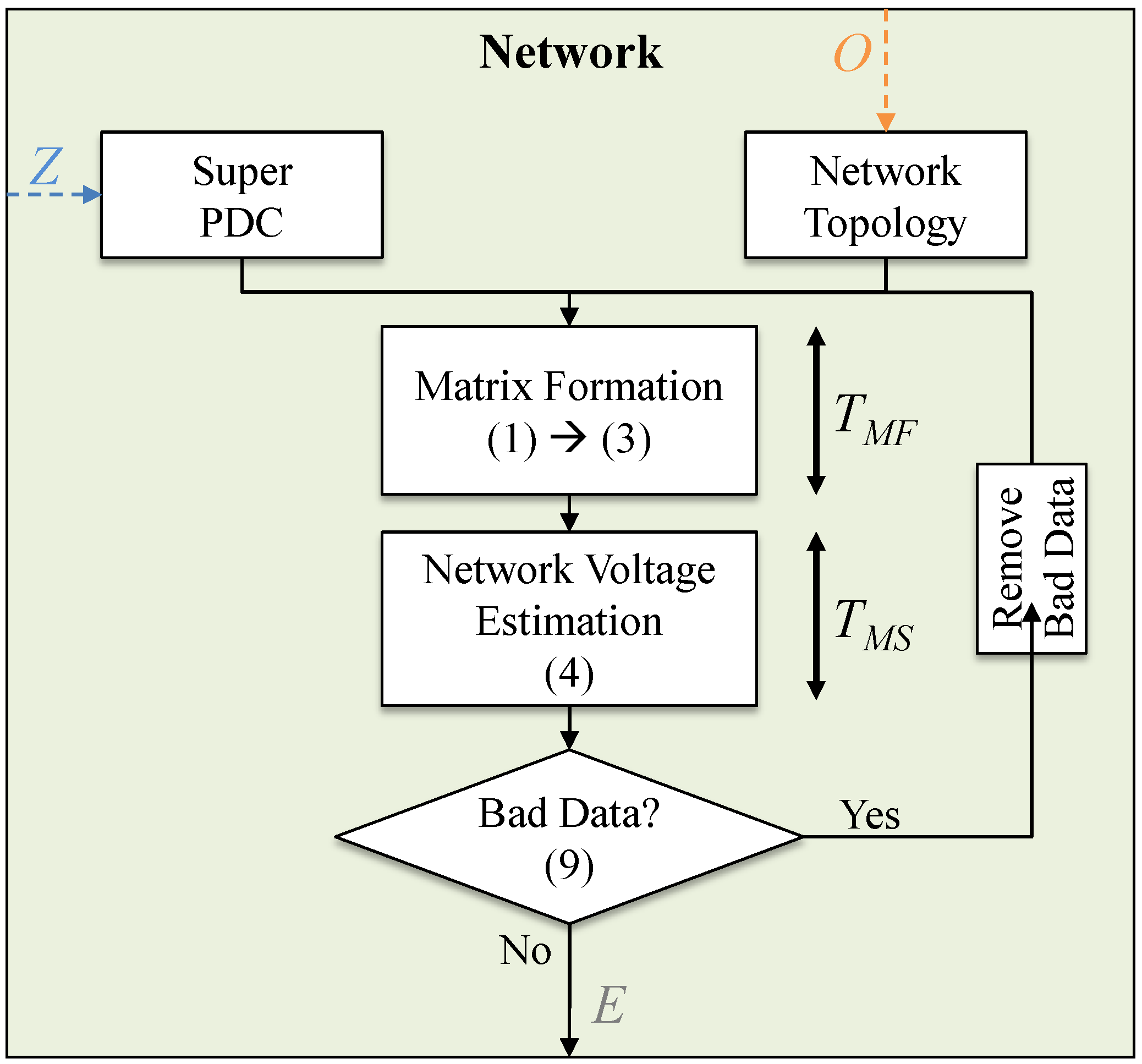
The network level will be utilized only if more bad measurements are flagged in the area level of the D-LSE after bypassing the substation level due to bad current measurements being detected. The enhanced network level integrated as the redundancy level for the area level of the D-LSE is shown in Figure 3 and elaborated in Figure 5. The is the computational time for matrix formation, and is the computational time for voltage estimation. Under bad data detection at the area level, a bad data flag is sent to the network level with the identified bad voltage measurements of the area. The network level will be based on the SOTA LSE formulation explained under Section 2.1. LSE will be formulated by intentionally neglecting the bad measurements detected, thus improving the estimation accuracy at the network level. The network topology can be retrieved from the H-TNTP Level 3 as shown in Figure 3.
3. Results and Discussion
This study considered two power system models, the modified two-area four-machine power system and the IEEE 68 bus power system, for implementing the D-LSE. All three level results are presented under topology changes and with bad data in the measurements for the modified two-area four-machine power system. For the IEEE 68 bus power system, the area-level and network-level results are presented. In the results tables, magnitude quantities are in per unit (pu) and indicated by “M (pu)”. Angle quantities are in degrees and indicated by “∠ °”. It is important to note that all the test results presented except for Section 3.1.1 and Section 3.2.1 have considered the fully connected topology of the networks.
The PMUs implemented in the RTDS simulation provided noise-free measurements, which are defined as the . The PMU measurement errors were regulated by the total vector error (TVE), which is the difference between the true phasor and the measured phasor. The standard maximum permissibility of the TVE is 1% [32]. To mimic the reality of the PMU measurements, a Gaussian white noise (GWN) was added to all at the simulator, thus defined as the . The GWN is a zero mean, user-defined level of variance noise addition to the signal using (10). To analyze the performance of the D-LSE, 5% of the noise level (variance) was considered in all experiments.
3.1. Modified Two-Area Four-Machine Power System (System 1)
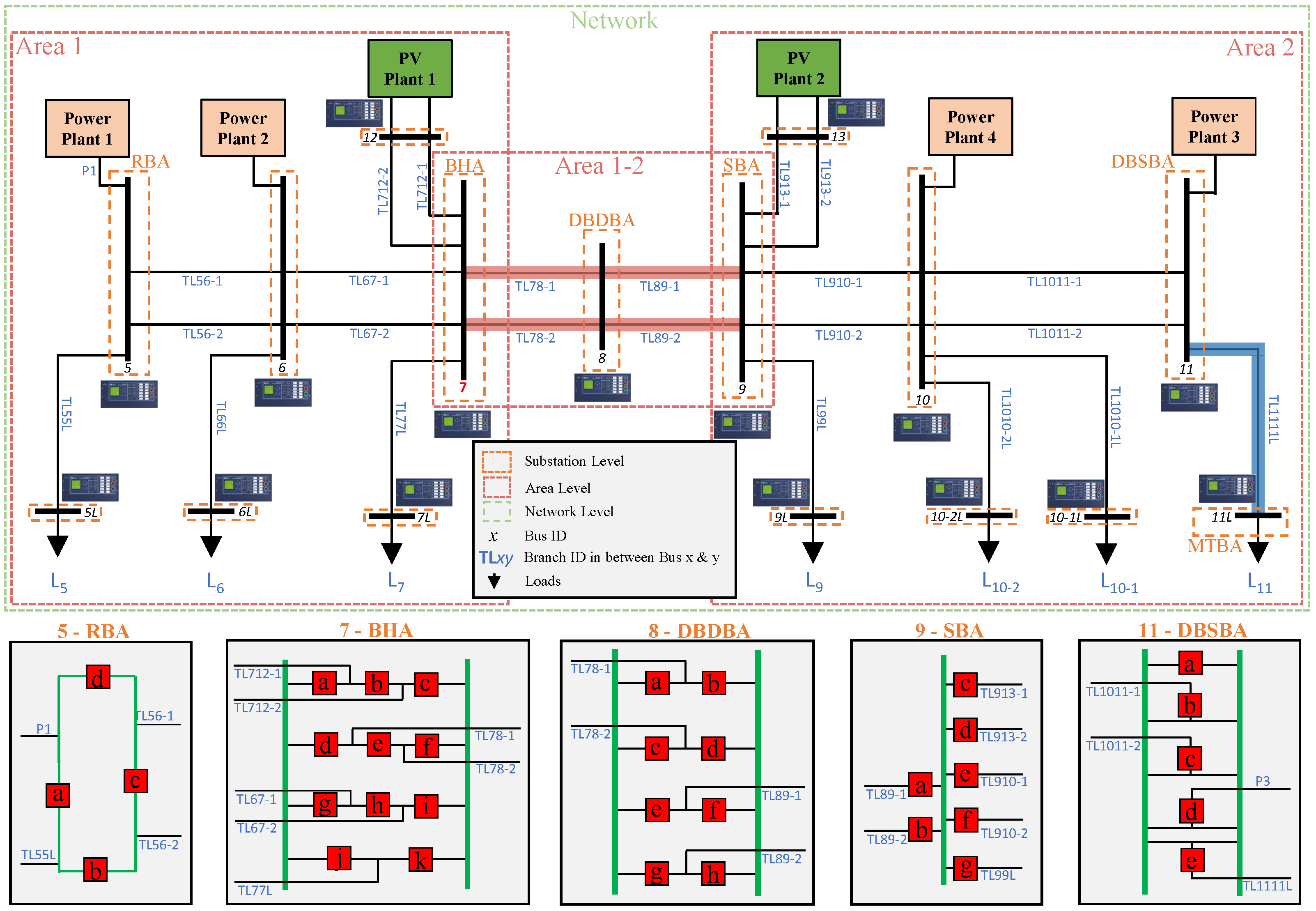
The benchmark two-area symmetric system consists of five buses and two machines in each area, thus representing each substation with a single bus. Two double-circuit tie lines connect the two areas through a tie-line bus. As shown in Figure 6, the modified two-area four-machine power system model consists of four conventional synchronous generator-based power plants and two additional solar power plants. The modified system contains seven loads at bus 5L, 6L, 7L, 9L, 10-1L, 10-2L, and 11L. The modified two-area four-machine power system model with all typically used substation arrangements has been considered [28]. All conventional generators were configured with turbine governors, automatic voltage regulators, and power system stabilizers. The simulation used the RSCAD FX 2.1 software on the Real-Time Digital Simulator (RTDS) [33]. RSCAD software PMUs were utilized as the measurement instruments for this study. Substation 9 was configured as a single bus arrangement (SBA). The SBA was the fundamental arrangement. The reliability of the SBA is low due to a lack of redundancy under breaker, isolator failure, or bus fault. Due to the lack of reliability, using the SBA is limited in practice. Substation 11L was configured as an MTBA. It is important to highlight that the MTBA acts as an SBA substation under normal operation (transfer bus on standby). Thus, the MTBA was not considered in the test cases. Substation 5 was configured as an RBA. Substation 11 was configured as a DBSBA. Substation 8 was configured as a DBDBA. Substation 7 was configured as a BHA. All other substations were configured as SBAs. Further information on each substation arrangement type can be found in [28]. PMUs were installed in each substation. Thus, the current phasor measurements of each branch connecting to any substation, node voltages, and breaker currents are available. The H-TNTP-PMU was implemented based on the node voltage and branch current phasor measurements from the PMUs. PMUs were collecting measurements at 30 Hz. Three areas were identified for the D-LSE area level in the modified two-area four-machine system, as shown in Figure 6. The selection was made since Substation 8 was not included in either Area 1 or Area 2. Thus, an additional area was designated to cover Substations 7, 8, and 9 as Area 1–2. Thus, D-LSE Area 1 included the 5G, 5, 5L, 6G, 6, 6L, 12, 7, and 7L substations. Area 1–2 included Substations 7, 8, and 9. Area 2 encompassed Substations 9, 13, 9L, 10G, 10, 10-1L, 10-2L, 11G, 11, and 11L.
The estimation’s accuracy assessment was based on error reduction. An error reduction factor (), calculated in (11), indicates the estimation accuracy as many-fold better than the measurement (noisy or bad) received. The is calculated by taking the inverse of the ratio of the absolute deviation between the estimated state and against the and . The is a unitless metric.
For accuracy, each test case voltage estimation was analyzed based on the . It is important to emphasize that the for the voltage estimation in SBA type was neglected, since the SBA only considers the available single bus voltage measurement as the estimated value from the weighted average. Furthermore, the SBA is an unreliable arrangement with limited practical use in the transmission network.
Table A1 presents the voltage estimates for all the substations under all three levels when independently operated. Furthermore, the for the voltage estimation of all three levels is shown in Table A1. Based on these results, the overall best accuracy under GWN was determined at the substation level.
3.1.1. Steady State with Gaussian White Noise for Topology Change
The D-LSE was tested for the topology changes detected by H-TNTP-PMU [28]. The topology changes from Topology S1A (fully connected network) considered for the modified two-area four-machine power system are Topology S1B and Topology S1C. The topology changes were selected in accordance with the test cases presented in [28], which elaborates the topology processing with H-TNTP-PMU. The topology was changed from Topology S1A to Topology S1B by removing TL1111L (single line outage). In the next experiment, the topology was changed from Topology S1A to Topology S1C by removing the double circuit tie lines, TL78-1, TL78-2, TL89-1, and TL89-2 (area separation), as shown in Figure 6. The H-TNTP-PMU outputs are shown in Figure 7. The pretopology change (from Topology S1A to Topology S1B or Topology S1C) matrix values are shown in orange, and the post-topology change values are shown in black. Table A1 presents the steady state voltage estimation for all three levels of the D-LSE in Topology S1A. Table 1 presents the steady state voltage estimation for all three levels in Topology S1B and Topology S1C. Due to the change in topology from Topology S1A to Topology S1B, Substation 11L was isolated. Due to the change in topology from Topology S1A to Topology S1C, Substation 8 was isolated. The performance of the three levels was tested during the transition from Topology S1A to Topology S1B and Topology S1A to Topology S1C. Furthermore, both topology transitions were conducted under SOTA TNTP, which typically updates the topology in 2 s to 5 s [15] and H-TNTP-PMU, which typically updates the topology in every PMU data frame [28]. The topology change experiment followed the setup shown in Figure 8. The substation-level, area-level, and network-level estimations for Substation 11, which were directly affected by Topology S1A to Topology S1B (TL1111L single line outage) transition, are shown in Figure 9 and Figure 10 under both H-TNTP-PMU and SOTA TNTP. The substation-level and area-level estimations for Substation 7, which were directly affected by Topology S1A to Topology S1C (area separation) transition, are shown in Figure 11 under both H-TNTP-PMU and SOTA TNTP. The start of the transition is indicated using “P”, and the SOTA TNTP detection of the topology change is indicated using “Q” in the Figure 9, Figure 10 and Figure 11. It can be seen that H-TNTP-PMU-based D-LSE and enhanced network-level LSE had an accurate estimation compared to the inefficient SOTA TNTP-based D-LSE and enhanced network-level LSE.
3.1.2. Steady State with Gaussian White Noise and Circuit Breaker Current Bad Data
The substation level of the D-LSE was tested for bad data. The bad data considered in the experiment were based on a common human error: connecting wires in reverse polarity. Thus, the bad data will be the reverse phasor of the received. At the substation, a circuit breaker current of bad data was applied. The current estimations of the substation level of the D-LSE for the BHA substation arrangement are presented in Table 2. The measurements highlighted in red are the bad data. The measurements highlighted in blue are the noisy measurements directly affected by the bad data. The normalized residual was used to detect and identify the bad data in the measurements. As it can be seen in Table 2, a single circuit breaker current bad data can negatively influence the related noisy measurements, which is the basis for handing over the voltage estimation to the subsequent level.
3.1.3. Steady State with Gaussian White Noise, Circuit Breaker Current Bad Data, and Injection Current Bad Data
The substation level of the D-LSE was tested for the inclusion of multiple bad data. A circuit breaker current with bad data and a single injection current with bad data were included at the substation. The current estimation of the substation level of the D-LSE for the BHA substation arrangement is presented in Table 3. As seen in Table 3, a single circuit breaker current and a single injection current with bad data significantly influenced the other related measurements and the substation-level estimation accuracy. Although the estimation was more accurate in the substation level under noisy conditions, as shown in the Table A1 results, the bad data highly deviated from the accuracy of the substation-level estimation. Thus, the state estimation was handed over to the area level under bad data detection at the substation level.
3.1.4. Steady State with Gaussian White Noise and Voltage Measurement Bad Data at Area Level
The substation level of the D-LSE identifies bad data through current estimation, which raises the substation bad data flag and informs the area level regarding the handing over process. The area level filters out the substation that detected bad data and conducts the LSE. Yet, there can be bad voltage phasor measurements at the area level, since substation level bad data detection is limited to the current measurements. Thus, bad data identification is conducted at the area level. The bad data considered were the reverse phasor of the voltage measurement in Substations 6 and 10. The results are presented in Table 4 for the area level and network level.
3.2. IEEE 68 Bus Power System (System 2)
The IEEE 68 bus power system model simulation and D-LSE implementation were based on the system shown in Figure 12. The IEEE 68 bus system demonstrates the scalability of the D-LSE. The IEEE 68 bus power system model comprises five areas with 16 conventional synchronous generators [34]. Area 1 consists of generators G1 to G9. Area 2 consists of generators G10 to G13. Areas 3, 4, and 5 contain a single generator per area, namely G14, G15, and G16. The D-LSE’s area level and network level were implemented on the IEEE 68 bus power system due to the limitations of implementing the substation arrangements of the simulation platform. This test system had no bus overlaps between areas, thus conveniently designating the area level with the buses in designated areas. Furthermore, the whole test system was considered a single entity at the network level.
The area level and network level were implemented into the IEEE 68 bus power system by considering all buses as SBAs, thus neglecting generator buses (Bus ID 1–16), since the generator buses were integrated into the generator module in the simulation model.
3.2.1. Steady State with Gaussian White Noise for Topology Change
The D-LSE was tested for the topology changes detected by H-TNTP-PMU [28] for the IEEE 68 bus system. The topology changes considered for the IEEE 68 bus system were Topology S2B and Topology S2C. The topologies were selected to avoid bus isolation, where pre- and postconditions are stable. Table A2 presents the steady state D-LSE voltage estimation for the area level and network level in Topology S2A. Table 5 presents the steady state voltage estimates for the D-LSE area level in Topology S2B and Topology S2C. In both topology changes, an alternative rerouting path was available. The topology was changed from Topology S2A (fully connected network) to Topology S2B by removing TL68-37 in Area 1, and the topology was changed from Topology S2B to Topology S2C subsequently by removing another single line in Area 2, TL36-34, as shown in Figure 12. The topology changes are shown in Figure 13.
3.3. Discussion
The computational efficiency was compared considering the analysis conducted in Table 6. The D-LSEs were evaluated for practical computational overhead with 50 trials on an Intel Xeon(R) Gold 3.3 GHz system with 63.7 GB RAM for all test cases present in Table A1 and Table A2. The execution time was calculated using (12). j is either the substation level, area level, or network level. It is important to note that this analysis did not account for communication latency or other processing delays. The computational time within the PMU data rate window as a percentage is shown in the last column of Table 6.
As a system, the modified two-area four-machine power system is small, and the computation time was less compared to the IEEE 68 bus system. Furthermore, the substation-level and the area-level computational times demonstrate the value of the distributed architecture. Since these two levels can be processed in parallel, the overall computational time can be minimized compared to the network level. This is important for new applications requiring PMU-based state estimation, where the smaller computation overhead is taken by TNTP [28] and LSE. Thus, it allows for higher computational flexibility for the new applications.
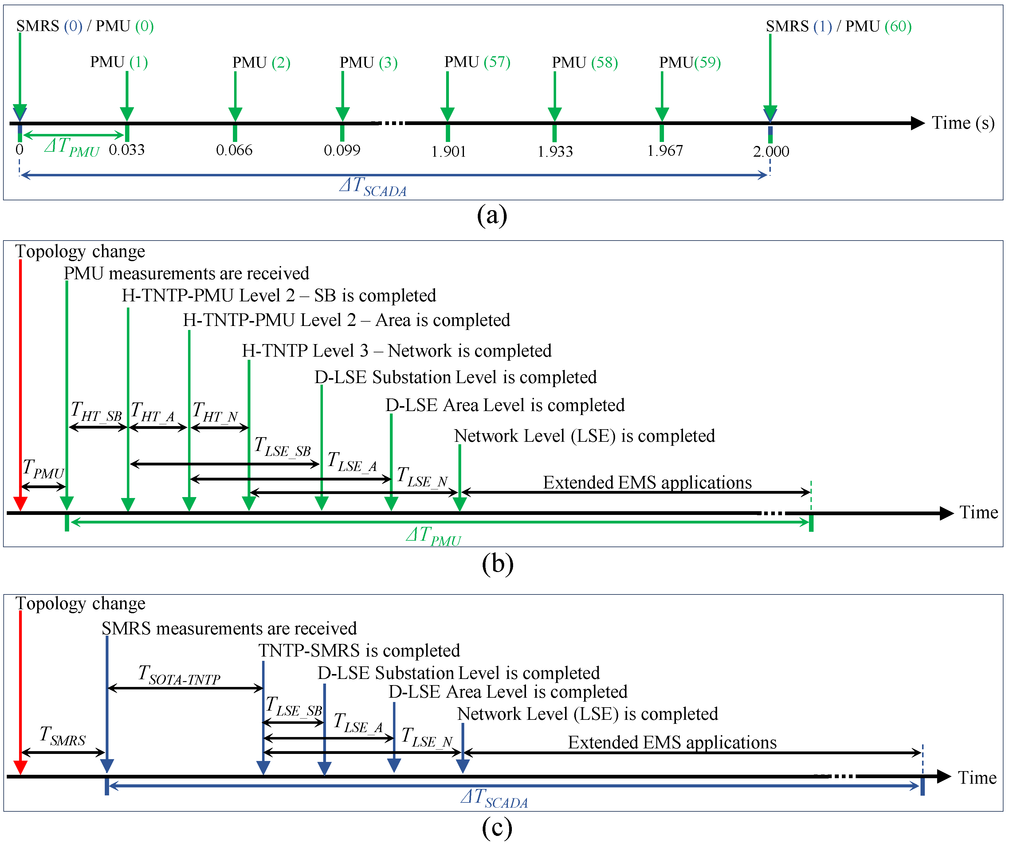
H-TNTP-PMU updates the network model in every PMU measurement frame, and SOTA-TNTP updates the network model in every SCADA measurement frame. The PMU and SMRS sampling at 30 Hz (every 33.33 ms) and every 2 s, respectively, is presented in a timeline as shown in Figure 14a. Due to the uncertainty of the instance, the network topology change occurred with respect to the PMU and SCADA samples collected; two possible scenarios in the topology identification-based flow can be defined as discussed in [28]. An extension to the same timeline interpretation, including three levels, is shown in Figure 14b,c. The delay between the instance the topology change occurred, and the next sample collected by the PMU and SCADA are defined as and , respectively. is the time taken to complete SOTA TNTP, while refers to the H-TNTP-PMU completion time, where k refers to either the substation level (SB), area level (A), or network level (N). refers to the time it takes to complete LSE in each level, where s is either the substation level (SB), area level (A), or network level (N). The time analysis shown in Table 7 was conducted for 50 trials for the Topology S1A to Topology S1B change discussed in Section 3.1.1. It is important to state that out of the 50 trials, of the time the was less than 33.33 ms.
A summarized comparison of the three levels of the D-LSE is presented in Table 8. It can be seen that the substation level’s highest computational time was less than that of the area level. Furthermore, the area level’s highest computational time was less than the network level’s. The robustness considers the ability to accurately estimate under noise (low: , medium: , and high: ), which is analyzed using the in Table A1 and Table A2. The resiliency considers estimation algorithm accuracy (low: and medium: ) under bad data in measurements, which are analyzed using the in Section 3.1.2, Section 3.1.3 and Section 3.1.4.
4. Conclusions
Modern power system operation is becoming complex and dynamic. Linear state estimation is a promising solution for state estimation with synchrophasor measurements. However, LSE is computationally inefficient for large power systems, and the state-of-the-art transmission network topology processing limits the true potential of LSE. An efficient, resilient, and robust multilevel distributed linear state estimation based on a hierarchical transmission network topology processing that updates the network model at the PMU rate has been presented in this paper. Using an efficient and reliable H-TNTP with synchrophasor data enables the practical implementation of a multilevel D-LSE for power systems of any scale. The typical results obtained with the multilevel D-LSE implemented on the modified IEEE two-area four-machine system model and the IEEE 68 bus system model demonstrate improved computational efficiency, resiliency against bad data, and robustness against noisy measurements. In addition, LSE at the network level integrated with the H-TNTP-PMU provides redundancy to the substation-level and area-level D-LSE. Future work includes investigating and developing security assessments for bulk power systems based on H-TNTP, multilevel D-LSE, and synchrophasor measurements with optimal usage.
Author Contributions
Conceptualization, D.M. and G.K.V.; methodology, D.M. and G.K.V.; software, D.M. and G.K.V.; validation, D.M. and G.K.V.; formal analysis, D.M. and G.K.V.; investigation, D.M. and G.K.V.; resources, G.K.V.; data curation, D.M.; writing—original draft preparation, D.M. and G.K.V.; writing—review and editing, G.K.V.; visualization, D.M. and G.K.V.; supervision, G.K.V.; project administration, G.K.V.; funding acquisition, G.K.V. All authors have read and agreed to the published version of the manuscript.
Funding
This study was supported in part by the National Science Foundation (NSF) of the United States, under grants CNS 2131070, ECCS 2234032 and CNS 2318612, and the Duke Energy Distinguished Professorship Endowment Fund. Any opinions, findings and conclusions, or recommendations expressed in this material are those of author(s) and do not necessarily reflect the views of NSF and Duke Energy.
Institutional Review Board Statement
Not applicable.
Informed Consent Statement
Not applicable.
Data Availability Statement
The datasets presented in this article are not readily available because the data are part of an ongoing study. Requests to access the datasets should be directed to the authors.
Conflicts of Interest
The authors declare no conflicts of interest.
Abbreviations
The following abbreviations are used in this manuscript:
| BBM | Bus branch mode |
| BHA | Breaker and half arrangement |
| CCN | Cellular computational network |
| DBDBA | Double bus double breaker arrangement |
| DBSBA | Double bus single breaker arrangement |
| D-LSE | Distributed linear state estimation |
| ERF | Error reduction factor |
| GWN | Gaussian white noise |
| H-TNTP | Hierarchical transmission network topology processing |
| H-TNTP-PMU | Synchrophasor-based hierarchical transmission network topology processing |
| KCL | Kirchhoff’s Current Law |
| LSE | Linear state estimation |
| MTBA | Main and transfer bus arrangement |
| NCM | Node connectivity matrix |
| PMU | Phasor measurement unit |
| RBA | Ring bus arrangement |
| RTDS | Real-Time Digital Simulator |
| SBA | Single bus arrangement |
| SCADA | Supervisory control and data acquisition |
| SMRS | Supervisory control and data acquisition system monitoring of relay signals |
| SOTA | State of the art |
| TNTP | Transmission network topology processing |
| TNTP-SMRS | Supervisory control and data acquisition system monitoring of relay signal-based transmission network topology processing |
| TVE | Total error vector |
Appendix A. Fully Connected Topology Voltage Estimation

Table A1.
Voltage estimation at the substation level, area level, and network level for modified two-area four-machine power system model (Topology S1A) under a steady state and the error reduction factor () analysis. Magnitude (“M”) is shown in pu, and the angle (∠) is in degrees (°).
Table A1.
Voltage estimation at the substation level, area level, and network level for modified two-area four-machine power system model (Topology S1A) under a steady state and the error reduction factor () analysis. Magnitude (“M”) is shown in pu, and the angle (∠) is in degrees (°).
| Substation | Measurement | True Value | Substation Level | Area Level | Network Level | ||||||||||||
|---|---|---|---|---|---|---|---|---|---|---|---|---|---|---|---|---|---|
| Voltage Estimation | Voltage Estimation | Voltage Estimation | |||||||||||||||
| ID | Type | M (pu) | ∠ ° | M (pu) | ∠ ° | M (pu) | ∠ ° | M (pu) | ∠ ° | M (pu) | ∠ ° | ||||||
| 5 | RBA | 1.000 | 33.908 | 1.031 | 34.009 | 1.027 | 33.990 | 8.30 | 5.19 | 1.018 | 33.964 | 2.34 | 2.24 | 1.014 | 33.952 | 1.83 | 1.75 |
| 5L | SBA | 1.041 | 30.715 | 1.027 | 30.588 | 1.041 | 30.715 | - | - | 1.033 | 30.635 | 2.50 | 2.67 | 1.036 | 30.653 | 1.63 | 1.95 |
| 6 | SBA | 1.074 | 34.620 | 1.030 | 34.761 | 1.074 | 34.620 | - | - | 1.046 | 34.711 | 2.73 | 2.81 | 1.052 | 34.687 | 1.99 | 1.90 |
| 6L | SBA | 0.992 | 32.673 | 1.027 | 32.707 | 0.992 | 32.673 | - | - | 1.012 | 32.693 | 2.38 | 2.40 | 1.006 | 32.686 | 1.62 | 1.58 |
| 12 | SBA | 1.020 | 34.793 | 1.035 | 34.927 | 1.020 | 34.793 | - | - | 1.028 | 34.877 | 2.23 | 2.71 | 1.027 | 34.849 | 1.90 | 1.73 |
| 7 | BHA | 1.063 | 34.692 | 1.033 | 34.559 | 1.039 | 34.573 | 5.73 | 9.78 | 1.044 | 34.613 | 2.82 | 2.47 | 1.052 | 34.633 | 1.62 | 1.80 |
| 7L | SBA | 1.012 | 33.933 | 1.032 | 33.992 | 1.012 | 33.933 | - | - | 1.023 | 33.966 | 2.28 | 2.32 | 1.020 | 33.961 | 1.69 | 1.93 |
| 8 | DBDBA | 1.043 | 31.449 | 1.042 | 31.550 | 1.042 | 31.532 | 7.80 | 5.75 | 1.043 | 31.511 | 2.46 | 2.61 | 1.043 | 31.487 | 2.00 | 1.61 |
| 13 | SBA | 1.030 | 29.066 | 1.033 | 29.046 | 1.030 | 29.066 | - | - | 1.032 | 29.055 | 2.29 | 2.33 | 1.032 | 29.059 | 1.88 | 1.56 |
| 9 | SBA | 1.016 | 28.611 | 1.032 | 28.662 | 1.016 | 28.611 | - | - | 1.026 | 28.644 | 2.84 | 2.86 | 1.022 | 28.632 | 1.56 | 1.72 |
| 9L | SBA | 0.999 | 27.765 | 1.031 | 27.629 | 0.999 | 27.765 | - | - | 1.019 | 27.683 | 2.68 | 2.52 | 1.015 | 27.697 | 1.94 | 1.99 |
| 10 | SBA | 0.983 | 28.658 | 1.029 | 28.551 | 0.983 | 28.658 | - | - | 1.010 | 28.596 | 2.40 | 2.37 | 1.005 | 28.618 | 1.89 | 1.60 |
| 10-1L | SBA | 1.015 | 25.902 | 1.025 | 25.810 | 1.015 | 25.902 | - | - | 1.021 | 25.848 | 2.81 | 2.46 | 1.020 | 25.866 | 1.93 | 1.64 |
| 10-2L | SBA | 1.029 | 25.861 | 1.025 | 25.800 | 1.029 | 25.861 | - | - | 1.027 | 25.823 | 2.30 | 2.61 | 1.027 | 25.836 | 1.75 | 1.68 |
| 11 | DBSBA | 0.982 | 28.470 | 1.031 | 28.427 | 1.022 | 28.437 | 5.41 | 4.05 | 1.011 | 28.444 | 2.49 | 2.56 | 1.005 | 28.451 | 1.86 | 1.76 |
| 11L | MTBA | 1.029 | 25.033 | 1.027 | 25.005 | 1.029 | 25.033 | - | - | 1.028 | 25.016 | 2.42 | 2.53 | 1.028 | 25.020 | 1.88 | 1.92 |
| Average | - | - | - | - | - | - | 6.81 | 6.19 | - | - | 2.50 | 2.53 | - | - | 1.81 | 1.76 | |
Table A2.
Voltage estimation at the area level and network level for IEEE 68 bus power system model (Topology S2A) under a steady state and the error reduction factor () analysis. Magnitude (“M”) is shown in pu, and the angle (∠) is in degrees (°).
Table A2.
Voltage estimation at the area level and network level for IEEE 68 bus power system model (Topology S2A) under a steady state and the error reduction factor () analysis. Magnitude (“M”) is shown in pu, and the angle (∠) is in degrees (°).
| Bus ID | Measurement | True Value | Area Level | Network Level | ||||||||
|---|---|---|---|---|---|---|---|---|---|---|---|---|
| Voltage Estimation | Voltage Estimation | |||||||||||
| M (pu) | ∠ ° | M (pu) | ∠ ° | M (pu) | ∠ ° | M (pu) | ∠ ° | |||||
| 17 | 1.044 | −5.747 | 1.025 | −5.728 | 1.033 | −5.736 | 2.38 | 2.40 | 1.037 | −5.738 | 1.59 | 1.93 |
| 18 | 0.992 | 42.644 | 0.993 | 42.752 | 0.993 | 42.705 | 2.77 | 2.31 | 0.993 | 42.683 | 1.84 | 1.56 |
| 19 | 1.021 | 24.180 | 1.052 | 24.099 | 1.040 | 24.133 | 2.73 | 2.34 | 1.032 | 24.145 | 1.54 | 1.76 |
| 20 | 0.978 | 22.578 | 0.992 | 22.673 | 0.986 | 22.639 | 2.43 | 2.76 | 0.985 | 22.614 | 1.91 | 1.61 |
| 21 | 1.072 | 22.065 | 1.036 | 22.135 | 1.051 | 22.109 | 2.36 | 2.70 | 1.056 | 22.100 | 1.75 | 1.99 |
| 22 | 1.072 | 26.733 | 1.052 | 26.797 | 1.059 | 26.770 | 2.57 | 2.33 | 1.064 | 26.758 | 1.59 | 1.65 |
| 23 | 1.058 | 26.411 | 1.047 | 26.510 | 1.051 | 26.470 | 2.67 | 2.47 | 1.054 | 26.449 | 1.68 | 1.60 |
| 24 | 1.034 | 19.771 | 1.044 | 19.691 | 1.040 | 19.719 | 2.44 | 2.85 | 1.038 | 19.734 | 1.93 | 1.87 |
| 25 | 1.099 | 20.103 | 1.063 | 20.038 | 1.077 | 20.067 | 2.60 | 2.24 | 1.086 | 20.073 | 1.59 | 1.83 |
| 26 | 1.095 | 19.052 | 1.060 | 19.011 | 1.074 | 19.028 | 2.61 | 2.36 | 1.078 | 19.035 | 1.95 | 1.67 |
| 27 | 1.060 | 17.402 | 1.048 | 17.349 | 1.053 | 17.369 | 2.35 | 2.66 | 1.054 | 17.377 | 1.90 | 1.87 |
| 28 | 1.082 | 22.071 | 1.054 | 22.136 | 1.065 | 22.110 | 2.52 | 2.50 | 1.071 | 22.096 | 1.61 | 1.64 |
| 29 | 1.083 | 24.779 | 1.052 | 24.767 | 1.065 | 24.772 | 2.46 | 2.60 | 1.071 | 24.774 | 1.68 | 1.81 |
| 30 | 1.018 | 11.592 | 1.051 | 11.535 | 1.037 | 11.560 | 2.47 | 2.30 | 1.030 | 11.568 | 1.56 | 1.70 |
| 31 | 1.054 | 14.147 | 1.055 | 14.170 | 1.055 | 14.161 | 2.73 | 2.65 | 1.055 | 14.158 | 1.87 | 2.00 |
| 32 | 1.047 | 15.483 | 1.048 | 15.417 | 1.048 | 15.440 | 2.32 | 2.81 | 1.048 | 15.459 | 1.81 | 1.56 |
| 33 | 1.063 | 11.612 | 1.051 | 11.561 | 1.056 | 11.581 | 2.39 | 2.56 | 1.058 | 11.589 | 1.62 | 1.87 |
| 34 | 1.109 | 5.660 | 1.059 | 5.664 | 1.078 | 5.663 | 2.68 | 2.31 | 1.088 | 5.662 | 1.72 | 1.77 |
| 35 | 1.025 | 5.583 | 1.007 | 5.598 | 1.015 | 5.591 | 2.34 | 2.34 | 1.017 | 5.589 | 1.91 | 1.60 |
| 36 | 1.002 | 1.652 | 1.036 | 1.654 | 1.024 | 1.653 | 2.69 | 2.35 | 1.016 | 1.653 | 1.68 | 1.76 |
| 37 | 1.031 | 18.141 | 1.043 | 18.139 | 1.039 | 18.140 | 2.64 | 2.76 | 1.036 | 18.141 | 1.66 | 1.59 |
| 38 | 1.070 | 13.748 | 1.053 | 13.803 | 1.059 | 13.778 | 2.71 | 2.22 | 1.064 | 13.770 | 1.61 | 1.68 |
| 39 | 1.004 | −6.462 | 0.997 | −6.440 | 1.000 | −6.449 | 2.25 | 2.29 | 1.000 | −6.454 | 1.99 | 1.62 |
| 40 | 1.114 | 20.919 | 1.070 | 20.920 | 1.089 | 20.920 | 2.27 | 2.31 | 1.098 | 20.920 | 1.58 | 1.60 |
| 41 | 1.013 | 49.487 | 1.000 | 49.514 | 1.005 | 49.502 | 2.62 | 2.26 | 1.008 | 49.499 | 1.60 | 1.78 |
| 42 | 1.034 | 43.548 | 0.999 | 43.515 | 1.012 | 43.527 | 2.69 | 2.62 | 1.017 | 43.535 | 1.95 | 1.62 |
| 43 | 0.957 | −5.967 | 1.007 | −5.945 | 0.985 | −5.954 | 2.30 | 2.41 | 0.978 | −5.958 | 1.74 | 1.63 |
| 44 | 0.992 | −5.952 | 1.007 | −5.951 | 1.000 | −5.952 | 2.27 | 2.78 | 0.999 | −5.952 | 1.79 | 1.75 |
| 45 | 0.971 | 5.434 | 1.009 | 5.419 | 0.994 | 5.425 | 2.47 | 2.37 | 0.987 | 5.428 | 1.69 | 1.67 |
| 46 | 1.040 | 14.695 | 1.031 | 14.628 | 1.035 | 14.654 | 2.41 | 2.64 | 1.036 | 14.662 | 1.93 | 1.98 |
| 47 | 1.070 | 13.256 | 1.073 | 13.297 | 1.072 | 13.283 | 2.51 | 2.79 | 1.072 | 13.277 | 1.76 | 1.98 |
| 48 | 1.052 | 15.070 | 1.077 | 15.131 | 1.068 | 15.104 | 2.58 | 2.27 | 1.064 | 15.093 | 1.91 | 1.63 |
| 49 | 1.021 | 17.771 | 1.012 | 17.720 | 1.016 | 17.738 | 2.39 | 2.77 | 1.017 | 17.746 | 1.73 | 1.99 |
| 50 | 1.054 | 23.026 | 1.004 | 22.934 | 1.024 | 22.973 | 2.58 | 2.38 | 1.036 | 22.983 | 1.58 | 1.87 |
| 51 | 1.045 | 9.623 | 1.012 | 9.619 | 1.026 | 9.620 | 2.43 | 2.62 | 1.031 | 9.621 | 1.79 | 1.83 |
| 52 | 1.044 | 17.203 | 1.041 | 17.261 | 1.042 | 17.238 | 2.60 | 2.51 | 1.043 | 17.231 | 1.63 | 1.93 |
| 53 | 1.106 | 12.611 | 1.057 | 12.661 | 1.078 | 12.643 | 2.37 | 2.84 | 1.086 | 12.631 | 1.68 | 1.65 |
| 54 | 1.021 | 18.602 | 1.054 | 18.605 | 1.040 | 18.604 | 2.37 | 2.31 | 1.035 | 18.603 | 1.69 | 1.69 |
| 55 | 0.994 | 16.894 | 1.042 | 16.939 | 1.023 | 16.919 | 2.47 | 2.28 | 1.014 | 16.914 | 1.72 | 1.80 |
| 56 | 0.999 | 17.625 | 1.026 | 17.686 | 1.014 | 17.662 | 2.24 | 2.52 | 1.012 | 17.649 | 1.93 | 1.67 |
| 57 | 1.059 | 18.134 | 1.023 | 18.110 | 1.038 | 18.120 | 2.37 | 2.35 | 1.046 | 18.123 | 1.58 | 1.86 |
| 58 | 1.039 | 18.760 | 1.024 | 18.739 | 1.031 | 18.747 | 2.23 | 2.56 | 1.033 | 18.751 | 1.79 | 1.81 |
| 59 | 1.038 | 16.439 | 1.016 | 16.372 | 1.026 | 16.400 | 2.29 | 2.37 | 1.030 | 16.412 | 1.58 | 1.67 |
| 60 | 0.994 | 15.807 | 1.017 | 15.764 | 1.007 | 15.780 | 2.34 | 2.62 | 1.003 | 15.788 | 1.61 | 1.81 |
| 61 | 1.077 | 7.573 | 1.035 | 7.595 | 1.050 | 7.586 | 2.84 | 2.31 | 1.061 | 7.584 | 1.59 | 1.97 |
| 62 | 0.988 | 21.344 | 1.030 | 21.241 | 1.011 | 21.277 | 2.24 | 2.81 | 1.007 | 21.295 | 1.82 | 1.90 |
| 63 | 0.999 | 20.428 | 1.027 | 20.388 | 1.015 | 20.402 | 2.35 | 2.82 | 1.010 | 20.410 | 1.64 | 1.80 |
| 64 | 1.043 | 20.386 | 1.069 | 20.382 | 1.060 | 20.384 | 2.80 | 2.59 | 1.054 | 20.385 | 1.79 | 1.76 |
| 65 | 1.036 | 20.567 | 1.028 | 20.593 | 1.031 | 20.583 | 2.85 | 2.43 | 1.032 | 20.577 | 1.89 | 1.59 |
| 66 | 1.071 | 19.183 | 1.028 | 19.100 | 1.043 | 19.136 | 2.79 | 2.32 | 1.054 | 19.146 | 1.65 | 1.80 |
| 67 | 0.997 | 18.353 | 1.025 | 18.302 | 1.015 | 18.322 | 2.82 | 2.58 | 1.009 | 18.330 | 1.73 | 1.82 |
| 68 | 1.037 | 19.510 | 1.039 | 19.518 | 1.039 | 19.514 | 2.56 | 2.30 | 1.038 | 19.514 | 1.65 | 2.00 |
| Average | - | - | - | - | - | - | 2.50 | 2.52 | - | - | 1.73 | 1.77 |
References
- Schweppe, F.C.; Wildes, J. Power System Static-State Estimation, Part I: Exact Model. IEEE Trans. Power Appar. Syst. 1970, PAS-89, 120–125. [Google Scholar] [CrossRef]
- Schweppe, F.C.; Rom, D.B. Power System Static-State Estimation, Part II: Approximate Model. IEEE Trans. Power Appar. Syst. 1970, PAS-89, 125–130. [Google Scholar] [CrossRef]
- Schweppe, F.C. Power System Static-State Estimation, Part III: Implementation. IEEE Trans. Power Appar. Syst. 1970, PAS-89, 130–135. [Google Scholar] [CrossRef]
- Cooper, A.; Bretas, A.; Meyn, S. Anomaly Detection in Power System State Estimation: Review and New Directions. Energies 2023, 16, 6678. [Google Scholar] [CrossRef]
- Zhang, G.; Gao, W.; Li, Y.; Guo, X.; Hu, P.; Zhu, J. Detection of False Data Injection Attacks in a Smart Grid Based on WLS and an Adaptive Interpolation Extended Kalman Filter. Energies 2023, 16, 7203. [Google Scholar] [CrossRef]
- PES-TR118. State Estimation for Integrated Energy Systems: Motivations, Advances, and Challenges; Technical Report; IEEE PES Energy Internet Coordinating Committee IEEE PES Working Group on Power System Static and Dynamic State Estimation: Blacksburg, VA, USA, 2023. [Google Scholar]
- Liang, J.; Venayagamoorthy, G.K.; Harley, R.G. Wide-Area Measurement Based Dynamic Stochastic Optimal Power Flow Control for Smart Grids With High Variability and Uncertainty. IEEE Trans. Smart Grid 2012, 3, 59–69. [Google Scholar] [CrossRef]
- Kar, S.; Hug, G.; Mohammadi, J.; Moura, J.M.F. Distributed State Estimation and Energy Management in Smart Grids: A Consensus + Innovations Approach. IEEE J. Sel. Top. Signal Process. 2014, 8, 1022–1038. [Google Scholar] [CrossRef]
- Li, X.; Balasubramanian, P.; Sahraei-Ardakani, M.; Abdi-Khorsand, M.; Hedman, K.W.; Podmore, R. Real-Time Contingency Analysis With Corrective Transmission Switching. IEEE Trans. Power Syst. 2017, 32, 2604–2617. [Google Scholar] [CrossRef]
- Abur, A.; Exposito, A.G. Power System State Estimation: Theory and Implementation; CRC Press: Boca Raton, FL, USA, 2004; Volume 24. [Google Scholar] [CrossRef]
- Jones, K.D. Synchrophasor-Only Dynamic State Estimation & Data Conditioning. Ph.D. Thesis, Virginia Polytechnic Institute and State University, Blacksburg, VA, USA, 2013. [Google Scholar]
- Phadke, A.; Thorp, J. Synchronized Phasor Measurements and Their Applications, 1st ed.; Springer: New York, NY, USA, 2008. [Google Scholar]
- Farrokhabadi, M.; Vanfretti, L. State-of-the-art of topology processors for EMS and PMU applications and their limitations. In Proceedings of the IECON 2012—38th Annual Conference on IEEE Industrial Electronics Society, Montreal, QC, Canada, 25–28 October 2012; pp. 1422–1427. [Google Scholar] [CrossRef]
- Cao, J.; Wan, Y.; Hua, H.; Yang, G. Performance modeling for data monitoring services in smart grid: A network calculus based approach. CSEE J. Power Energy Syst. 2020, 6, 610–618. [Google Scholar] [CrossRef]
- Kong, X.; Chen, Y.; Xu, T.; Wang, C.; Yong, C.; Li, P.; Yu, L. A Hybrid State Estimator Based on SCADA and PMU Measurements for Medium Voltage Distribution System. Appl. Sci. 2018, 8, 1527. [Google Scholar] [CrossRef]
- Zhao, J.; Gómez-Expósito, A.; Netto, M.; Mili, L.; Abur, A.; Terzija, V.; Kamwa, I.; Pal, B.; Singh, A.K.; Qi, J.; et al. Power System Dynamic State Estimation: Motivations, Definitions, Methodologies, and Future Work. IEEE Trans. Power Syst. 2019, 34, 3188–3198. [Google Scholar] [CrossRef]
- Zhao, J.; Mili, L.; La Scala, M. A robust hybrid power system state estimator with unknown measurement noise. In Advances in Electric Power and Energy; John Wiley & Sons, Ltd.: Hoboken, NJ, USA, 2020; Chapter 8; pp. 231–253. [Google Scholar] [CrossRef]
- Xie, L.; Choi, D.H.; Kar, S.; Poor, H.V. Fully Distributed State Estimation for Wide-Area Monitoring Systems. IEEE Trans. Smart Grid 2012, 3, 1154–1169. [Google Scholar] [CrossRef]
- Kekatos, V.; Giannakis, G.B. Distributed Robust Power System State Estimation. IEEE Trans. Power Syst. 2013, 28, 1617–1626. [Google Scholar] [CrossRef]
- Korres, G.N. A Distributed Multiarea State Estimation. IEEE Trans. Power Syst. 2011, 26, 73–84. [Google Scholar] [CrossRef]
- Zhu, H.; Giannakis, G.B. Power System Nonlinear State Estimation Using Distributed Semidefinite Programming. IEEE J. Sel. Top. Signal Process. 2014, 8, 1039–1050. [Google Scholar] [CrossRef]
- Guo, Y.; Wu, W.; Zhang, B.; Sun, H. A distributed state estimation method for power systems incorporating linear and nonlinear models. Int. J. Electr. Power Energy Syst. 2015, 64, 608–616. [Google Scholar] [CrossRef]
- Jones, K.D.; Thorp, J.S.; Gardner, R.M. Three-phase linear state estimation using Phasor Measurements. In Proceedings of the 2013 IEEE Power Energy Society General Meeting, Vancouver, BC, Canada, 21–25 July 2013; pp. 1–5. [Google Scholar] [CrossRef]
- Vanfretti, L.; Chow, J.H.; Sarawgi, S.; Fardanesh, B. A Phasor-Data-Based State Estimator Incorporating Phase Bias Correction. IEEE Trans. Power Syst. 2011, 26, 111–119. [Google Scholar] [CrossRef]
- Yang, T.; Sun, H.; Bose, A. Two-level PMU-based linear state estimator. In Proceedings of the 2009 IEEE/PES Power Systems Conference and Exposition, Washington, DC, USA, 15–18 March 2009; pp. 1–6. [Google Scholar] [CrossRef]
- Yang, T.; Sun, H.; Bose, A. Transition to a Two-Level Linear State Estimator—Part I: Architecture. IEEE Trans. Power Syst. 2011, 26, 46–53. [Google Scholar] [CrossRef]
- Yang, T.; Sun, H.; Bose, A. Transition to a Two-Level Linear State Estimator—Part II: Algorithm. IEEE Trans. Power Syst. 2011, 26, 54–62. [Google Scholar] [CrossRef]
- Madurasinghe, D.; Venayagamoorthy, G.K. An Efficient and Reliable Electric Power Transmission Network Topology Processing. IEEE Access 2023, 11, 127956–127973. [Google Scholar] [CrossRef]
- Biswal, C.; Sahu, B.K.; Mishra, M.; Rout, P.K. Real-Time Grid Monitoring and Protection: A Comprehensive Survey on the Advantages of Phasor Measurement Units. Energies 2023, 16, 4054. [Google Scholar] [CrossRef]
- Wu, L.; Venayagamoorthy, G.K.; Gao, J. Online Steady-State Security Awareness Using Cellular Computation Networks and Fuzzy Techniques. Energies 2021, 14, 148. [Google Scholar] [CrossRef]
- McDonald, J.D. Electric Power Substations Engineering, 3rd ed.; CRC Press: Boca Raton, FL, USA, 2012. [Google Scholar]
- Zhang, X.; Lu, C.; Lin, J.; Wang, Y. Experimental test of PMU measurement errors and the impact on load model parameter identification. IET Gener. Transm. Distrib. 2020, 14, 4593–4604. [Google Scholar] [CrossRef]
- RTDS Technologies Inc. Real-Time Digital Power System Simulation. Available online: https://www.rtds.com (accessed on 15 April 2024).
- Bikash Pal, B.C. Robust Control in Power Systems; Springer: New York, NY, USA, 2005. [Google Scholar]
Figure 1.
Distributed linear state estimation (D-LSE) integrated with the state-of-the-art (SOTA) linear state estimation (LSE). The ‘orange-line’ blocks present the contribution of this work.
Figure 1.
Distributed linear state estimation (D-LSE) integrated with the state-of-the-art (SOTA) linear state estimation (LSE). The ‘orange-line’ blocks present the contribution of this work.

Figure 2.
Log-scaled number of algebraic operations and execution time for LSE procedures (excluding H-TNTP computation).
Figure 2.
Log-scaled number of algebraic operations and execution time for LSE procedures (excluding H-TNTP computation).

Figure 3.
Flow diagram of the proposed distributed LSE (D-LSE), including network level integrated with hierarchical transmission network topology processing based on synchrophasor measurements (H-TNTP-PMU) [28].
Figure 3.
Flow diagram of the proposed distributed LSE (D-LSE), including network level integrated with hierarchical transmission network topology processing based on synchrophasor measurements (H-TNTP-PMU) [28].

Figure 4.
(a) Flow diagram of the proposed D-LSE at the substation level considering Substation P as an example. LSE procedure flow paths A and B, measurement communication path W, and H-TNTP-PMU topology path M are referred to in Figure 3. (b) Flow diagram of the proposed D-LSE at the area level considering Area S as an example. LSE procedure flow paths C and D, measurement communication paths X and Y, and H-TNTP-PMU topology path N referred to in Figure 3.

Figure 5.
Flow diagram of the network level. LSE procedure flow path E, measurement communication path Z, and H-TNTP-PMU topology path O are referred to in Figure 3.
Figure 5.
Flow diagram of the network level. LSE procedure flow path E, measurement communication path Z, and H-TNTP-PMU topology path O are referred to in Figure 3.

Figure 6.
Modified two-area four-machine power system model indicating substation level, area level, and network level. Topology was changed from Topology S1A (fully connected network) to Topology S1B by removing TL1111L (single line outage), which is indicated in blue. Topology was changed from Topology S1A to Topology S1C by removing two double circuit tie lines, TL78-1, TL78-2, TL89-1, and TL89-2 (area separation), which is shown in red. Breakers in each substation are identified with lowercase letters.

Figure 7.
The topology change detected by H-TNTP-PMU Level 2-SB, Level 2-Area, and Level 3 [28]. (a) Topology S1A (fully connected) to Topology S1B. (b) Topology S1A to Topology S1C.
Figure 7.
The topology change detected by H-TNTP-PMU Level 2-SB, Level 2-Area, and Level 3 [28]. (a) Topology S1A (fully connected) to Topology S1B. (b) Topology S1A to Topology S1C.

Figure 8.
Experiment setup for executing D-LSE for H-TNTP-PMU and SOTA TNTP.

Figure 9.
Voltage phasor magnitude estimation of the Substation 11 during the Topology S1A to Topology S1B change. (a) Substation level. (b) Area level. (c) Network level.
Figure 9.
Voltage phasor magnitude estimation of the Substation 11 during the Topology S1A to Topology S1B change. (a) Substation level. (b) Area level. (c) Network level.

Figure 10.
Voltage phasor angle estimation of the Substation 11 during the Topology S1A to Topology S1B change. (a) Substation level. (b) Area level. (c) Network level.
Figure 10.
Voltage phasor angle estimation of the Substation 11 during the Topology S1A to Topology S1B change. (a) Substation level. (b) Area level. (c) Network level.

Figure 11.
Voltage estimation of Substation 7 during the Topology S1A to Topology S1C change. (a) Substation level. (b) Area level.
Figure 11.
Voltage estimation of Substation 7 during the Topology S1A to Topology S1C change. (a) Substation level. (b) Area level.

Figure 12.
IEEE 68 bus benchmark system [34] indicating D-LSE area level and network level. Topology was changed from Topology S2A (fully connected network) to Topology S2B by removing TL68-37, which is indicated in blue. Topology was changed from Topology S2B to Topology S2C by removing TL36-34, which is shown in red.

Figure 13.
The topology change detected by H-TNTP-PMU Level 2-Area and H-TNTP Level 3 [28]. (a) Topology S2A (fully connected) to Topology S2B. (b) Topology S2B to Topology S2C.
Figure 13.
The topology change detected by H-TNTP-PMU Level 2-Area and H-TNTP Level 3 [28]. (a) Topology S2A (fully connected) to Topology S2B. (b) Topology S2B to Topology S2C.

Figure 14.
(a) The PMU and SMRS sampling timeline. (b) The timeline for estimation utilizing H-TNTP-PMU as the topology processor. (c) The timeline for estimation utilizing SOTA TNTP as the topology processor.
Figure 14.
(a) The PMU and SMRS sampling timeline. (b) The timeline for estimation utilizing H-TNTP-PMU as the topology processor. (c) The timeline for estimation utilizing SOTA TNTP as the topology processor.

Table 1.
Voltage estimation from the substation level, area level, and network level for modified two-area four-machine power system model under a steady state for Topology S1B (single line outage) and Topology S1C (area separation). Magnitude (“M”) is shown in pu, and the angle (∠) is in degrees (°).
| ID | Topology S1B | Topology S1C | ||||||||||||||||||
|---|---|---|---|---|---|---|---|---|---|---|---|---|---|---|---|---|---|---|---|---|
| Measurement | True Value | Substation Level | Area Level | Network Level | Measurement | True Value | Substation Level | Area Level | Network Level | |||||||||||
| M (pu) | ∠ ° | M (pu) | ∠ ° | M (pu) | ∠ ° | M (pu) | ∠ ° | M (pu) | ∠ ° | M (pu) | ∠ ° | M (pu) | ∠ ° | M (pu) | ∠ ° | M (pu) | ∠ ° | M (pu) | ∠ ° | |
| 5 | 1.058 | 34.723 | 1.031 | 34.608 | 1.036 | 34.630 | 1.041 | 34.652 | 1.046 | 34.678 | 1.024 | −17.281 | 1.027 | −17.359 | 1.027 | −17.340 | 1.026 | −17.331 | 1.025 | −17.317 |
| 5L | 1.013 | 30.516 | 1.026 | 30.494 | 1.013 | 30.516 | 1.020 | 30.504 | 1.019 | 30.508 | 0.973 | −13.188 | 1.022 | −13.214 | 0.973 | −13.188 | 1.002 | −13.203 | 0.991 | −13.199 |
| 6 | 1.072 | 35.226 | 1.029 | 35.107 | 1.072 | 35.226 | 1.047 | 35.155 | 1.056 | 35.182 | 1.051 | −18.360 | 1.024 | −18.283 | 1.051 | −18.360 | 1.036 | −18.317 | 1.038 | −18.327 |
| 6L | 1.034 | 32.234 | 1.026 | 32.361 | 1.034 | 32.234 | 1.029 | 32.312 | 1.030 | 32.289 | 0.997 | −15.488 | 1.021 | −15.506 | 0.997 | −15.488 | 1.011 | −15.499 | 1.007 | −15.496 |
| 12 | 1.063 | 35.144 | 1.034 | 35.161 | 1.063 | 35.144 | 1.046 | 35.154 | 1.049 | 35.152 | 1.059 | −18.658 | 1.027 | −18.614 | 1.059 | −18.658 | 1.041 | −18.630 | 1.047 | −18.637 |
| 7 | 0.999 | 34.717 | 1.033 | 34.784 | 1.027 | 34.769 | 1.020 | 34.760 | 1.014 | 34.746 | 1.001 | −18.318 | 1.026 | −18.240 | 1.022 | −18.249 | 1.017 | −18.270 | 1.011 | −18.288 |
| 7L | 1.029 | 33.909 | 1.031 | 33.972 | 1.029 | 33.909 | 1.030 | 33.946 | 1.030 | 33.939 | 0.999 | −17.434 | 1.024 | −17.415 | 0.999 | −17.434 | 1.013 | −17.423 | 1.010 | −17.426 |
| 8 | 1.012 | 31.734 | 1.041 | 31.758 | 1.036 | 31.755 | 1.029 | 31.749 | 1.023 | 31.743 | - | - | - | - | - | - | - | - | - | - |
| 13 | 1.002 | 29.097 | 1.032 | 29.241 | 1.002 | 29.097 | 1.020 | 29.188 | 1.017 | 29.157 | 1.051 | 27.920 | 1.033 | 27.845 | 1.051 | 27.920 | 1.040 | 27.875 | 1.043 | 27.883 |
| 9 | 1.006 | 28.931 | 1.031 | 28.870 | 1.006 | 28.931 | 1.020 | 28.892 | 1.015 | 28.902 | 1.053 | 27.391 | 1.031 | 27.471 | 1.053 | 27.391 | 1.040 | 27.442 | 1.044 | 27.424 |
| 9L | 1.067 | 27.753 | 1.028 | 27.785 | 1.067 | 27.753 | 1.044 | 27.773 | 1.049 | 27.765 | 1.022 | 26.307 | 1.029 | 26.389 | 1.022 | 26.307 | 1.026 | 26.353 | 1.025 | 26.342 |
| 10 | 1.064 | 28.704 | 1.028 | 28.785 | 1.064 | 28.704 | 1.044 | 28.754 | 1.048 | 28.735 | 1.034 | 27.769 | 1.028 | 27.658 | 1.034 | 27.769 | 1.030 | 27.698 | 1.031 | 27.726 |
| 10-1L | 1.047 | 25.937 | 1.024 | 26.029 | 1.047 | 25.937 | 1.033 | 25.992 | 1.037 | 25.982 | 1.044 | 24.986 | 1.025 | 24.908 | 1.044 | 24.986 | 1.033 | 24.936 | 1.036 | 24.955 |
| 10-2L | 0.991 | 25.909 | 1.024 | 26.029 | 0.991 | 25.909 | 1.010 | 25.981 | 1.007 | 25.957 | 0.996 | 24.966 | 1.025 | 24.908 | 0.996 | 24.966 | 1.014 | 24.930 | 1.007 | 24.941 |
| 11 | 1.043 | 29.495 | 1.031 | 29.381 | 1.033 | 29.410 | 1.036 | 29.426 | 1.038 | 29.447 | 1.036 | 28.036 | 1.031 | 27.978 | 1.032 | 27.991 | 1.033 | 28.000 | 1.034 | 28.007 |
| 11L | - | - | - | - | - | - | - | - | - | - | 0.983 | 24.526 | 1.027 | 24.555 | 0.983 | 24.526 | 1.009 | 24.545 | 1.004 | 24.539 |
Table 2.
D-LSE of the substation-level current estimation results for Substation 7 (BHA) with circuit breaker c (CB c) current bad data. Magnitude (“M”) is shown in pu, and the angle (∠) is in degrees (°).
Table 2.
D-LSE of the substation-level current estimation results for Substation 7 (BHA) with circuit breaker c (CB c) current bad data. Magnitude (“M”) is shown in pu, and the angle (∠) is in degrees (°).
| Current | Measurement | True Value | Substation Level | NR | |||||
|---|---|---|---|---|---|---|---|---|---|
| Current Estimation | |||||||||
| M (pu) | ∠ ° | M (pu) | ∠ ° | M (pu) | ∠ ° | ||||
| CB a | 0.273 | 76.108 | 0.277 | 75.412 | 0.274 | 76.955 | 1.37 | 0.45 | 11.43 |
| CB b | 0.019 | 87.367 | 0.001 | −93.523 | 0.016 | −56.099 | 1.18 | 4.83 | 20.95 |
| CB c | 0.287 | 74.055 | 0.277 | −104.604 | 0.068 | −98.092 | 0.05 | 27.44 | 32.38 |
| CB d | 0.665 | −95.414 | 0.683 | −94.674 | 0.672 | −94.559 | 1.69 | 6.43 | 2.99 |
| CB e | 0.045 | 83.710 | 0.000 | −95.544 | 0.020 | 55.465 | 2.23 | 1.19 | 4.35 |
| CB f | 0.690 | 85.915 | 0.683 | 85.326 | 0.680 | 86.016 | 2.55 | 0.85 | 1.56 |
| CB g | 0.652 | 89.972 | 0.665 | 90.739 | 0.653 | 89.762 | 1.11 | 0.78 | 0.41 |
| CB h | 0.007 | 96.894 | 0.000 | −94.520 | 0.005 | 85.032 | 1.33 | 1.07 | 0.31 |
| CB i | 0.675 | −89.509 | 0.665 | −89.262 | 0.672 | −89.405 | 1.47 | 1.73 | 0.47 |
| CB j | 0.268 | −91.236 | 0.253 | −91.972 | 0.264 | −90.679 | 1.33 | 0.57 | 0.69 |
| CB k | 0.243 | 88.654 | 0.253 | 88.030 | 0.247 | 88.361 | 1.71 | 1.89 | 0.69 |
| TL127-1 | 0.279 | 77.299 | 0.278 | 75.455 | - | - | - | - | 11.43 |
| TL127-2 | 0.308 | 75.560 | 0.278 | 75.455 | - | - | - | - | 32.38 |
| TL78-1 | 0.682 | −92.871 | 0.682 | −94.675 | - | - | - | - | 2.99 |
| TL78-2 | 0.683 | −93.321 | 0.682 | −94.675 | - | - | - | - | 1.56 |
| TL67-1 | 0.648 | 89.479 | 0.665 | 90.738 | - | - | - | - | 0.41 |
| TL67-2 | 0.662 | 90.639 | 0.665 | 90.738 | - | - | - | - | 0.47 |
| TL77L | 0.504 | −90.705 | 0.505 | −91.971 | - | - | - | - | 0.69 |
| Average | - | - | - | - | - | - | 1.46 | 4.29 | - |
Table 3.
D-LSE of the substation-level current estimation results for Substation 7 (BHA) with circuit breaker c (CB c) current and injection current from TL67-2 bad data. Magnitude (“M”) is shown in pu, and the angle (∠) is in degrees (°).
Table 3.
D-LSE of the substation-level current estimation results for Substation 7 (BHA) with circuit breaker c (CB c) current and injection current from TL67-2 bad data. Magnitude (“M”) is shown in pu, and the angle (∠) is in degrees (°).
| Current | True Value | Measurement | Substation Level | NR | |||||
|---|---|---|---|---|---|---|---|---|---|
| Current Estimation | |||||||||
| M (pu) | ∠ ° | M (pu) | ∠ ° | M (pu) | ∠ ° | ||||
| CB a | 0.277 | 75.412 | 0.264 | 75.867 | 0.208 | 75.505 | 0.19 | 4.88 | 8.30 |
| CB b | 0.001 | −93.523 | 0.014 | −95.401 | 0.138 | 76.403 | 0.10 | 0.01 | 22.65 |
| CB c | 0.277 | −104.604 | 0.274 | 77.099 | 0.067 | −45.902 | 0.01 | 3.10 | 30.95 |
| CB d | 0.683 | −94.674 | 0.688 | −95.953 | 0.685 | −94.962 | 2.94 | 4.43 | 2.19 |
| CB e | 0.000 | −95.544 | 0.015 | 84.897 | 0.013 | −5.012 | 1.15 | 1.99 | 2.93 |
| CB f | 0.683 | 85.326 | 0.675 | 83.953 | 0.687 | 84.050 | 1.82 | 1.08 | 1.69 |
| CB g | 0.665 | 90.739 | 0.666 | 89.695 | 0.845 | 89.758 | 0.01 | 1.06 | 26.70 |
| CB h | 0.000 | −94.520 | 0.022 | 85.946 | 0.348 | 90.385 | 0.06 | 0.98 | 48.71 |
| CB i | 0.665 | −89.262 | 0.684 | −90.771 | 0.179 | −94.176 | 0.04 | 0.31 | 75.41 |
| CB j | 0.253 | −91.972 | 0.261 | −90.571 | 0.251 | −91.487 | 6.14 | 2.89 | 1.62 |
| CB k | 0.253 | 88.030 | 0.269 | 89.445 | 0.259 | 88.558 | 2.47 | 2.68 | 1.62 |
| TL127-1 | 0.278 | 75.455 | 0.291 | 75.604 | - | - | - | - | 8.30 |
| TL127-2 | 0.278 | 75.455 | 0.279 | 76.849 | - | - | - | - | 30.95 |
| TL78-1 | 0.682 | −94.675 | 0.692 | −92.515 | - | - | - | - | 2.19 |
| TL78-2 | 0.682 | −94.675 | 0.698 | −95.079 | - | - | - | - | 1.69 |
| TL67-1 | 0.665 | 90.738 | 0.676 | 89.497 | - | - | - | - | 26.70 |
| TL67-2 | 0.665 | 90.738 | 0.675 | -88.369 | - | - | - | - | 75.41 |
| TL77L | 0.505 | −91.971 | 0.501 | −91.942 | - | - | - | - | 1.62 |
| Average | - | - | - | - | - | - | 1.36 | 2.13 | - |
Table 4.
Voltage estimation from the area level and network level for modified two-area four-machine power system model under a steady state with bad voltage data in Substations 6 and 10 (not detected by the substation level) included in area level. Magnitude (“M”) is shown in pu, and the angle (∠) is in degrees (°).
| Substation | Measurement | True Value | Area Level | NR | Network Level | |||||||||
|---|---|---|---|---|---|---|---|---|---|---|---|---|---|---|
| Voltage Estimation | Voltage Estimation | |||||||||||||
| ID | Type | M (pu) | ∠ ° | M (pu) | ∠ ° | M (pu) | ∠ ° | M (pu) | ∠ ° | |||||
| 5 | RBA | 0.987 | 34.485 | 1.031 | 34.009 | 1.014 | 34.043 | 2.48 | 14.21 | 0.93 | 1.011 | 34.085 | 2.15 | 6.31 |
| 5L | SBA | 1.021 | 28.265 | 1.027 | 30.588 | 1.023 | 29.625 | 1.60 | 2.41 | 1.61 | 1.022 | 29.319 | 1.12 | 1.83 |
| 6 | SBA | 1.037 | −144.806 | 1.030 | 34.761 | 1.036 | −55.029 | 1.21 | 2.00 | 43.41 | 1.031 | 28.187 | 5.23 | 27.31 |
| 6L | SBA | 0.983 | 33.094 | 1.027 | 32.707 | 1.034 | 32.939 | 6.84 | 1.67 | 3.04 | 1.032 | 33.496 | 9.52 | 0.49 |
| 12 | SBA | 1.021 | 34.723 | 1.035 | 34.927 | 1.030 | 34.653 | 2.69 | 0.74 | 2.26 | 1.024 | 34.474 | 1.36 | 0.45 |
| 7 | BHA | 1.056 | 32.988 | 1.033 | 34.559 | 1.037 | 33.983 | 6.39 | 2.73 | 2.61 | 1.038 | 39.849 | 4.51 | 0.30 |
| 7L | SBA | 1.007 | 34.388 | 1.032 | 33.992 | 1.023 | 34.068 | 2.85 | 5.18 | 1.33 | 1.015 | 34.084 | 1.45 | 4.30 |
| 8 | DBDBA | 1.026 | 32.697 | 1.042 | 31.550 | 1.035 | 31.935 | 2.38 | 2.98 | 0.93 | 1.037 | 31.849 | 3.09 | 3.83 |
| 13 | SBA | 1.042 | 30.516 | 1.033 | 29.046 | 1.031 | 29.419 | 4.25 | 3.94 | 3.14 | 1.039 | 29.295 | 1.52 | 5.91 |
| 9 | SBA | 1.011 | 28.623 | 1.032 | 28.662 | 1.022 | 28.824 | 2.03 | 0.24 | 2.23 | 1.015 | 28.692 | 1.23 | 1.31 |
| 9L | SBA | 1.010 | 27.395 | 1.031 | 27.629 | 1.013 | 27.796 | 1.16 | 1.40 | 3.41 | 1.011 | 27.697 | 1.06 | 3.45 |
| 10 | SBA | 1.040 | −151.395 | 1.029 | 28.551 | 1.020 | −61.421 | 1.31 | 2.00 | 38.40 | 1.024 | 17.935 | 2.34 | 16.95 |
| 10-1L | SBA | 1.036 | 24.548 | 1.025 | 25.810 | 1.018 | 25.127 | 1.49 | 1.85 | 1.61 | 1.033 | 25.238 | 1.34 | 2.21 |
| 10-2L | SBA | 1.013 | 27.319 | 1.025 | 25.800 | 1.023 | 25.267 | 6.78 | 2.85 | 2.26 | 1.019 | 25.015 | 1.88 | 1.94 |
| 11 | DBSBA | 1.005 | 28.381 | 1.031 | 28.427 | 1.022 | 28.492 | 2.75 | 0.71 | 2.20 | 1.017 | 28.244 | 1.86 | 0.25 |
| 11L | MTBA | 1.003 | 24.564 | 1.027 | 25.005 | 1.033 | 25.589 | 4.25 | 0.76 | 1.04 | 1.039 | 25.342 | 2.12 | 1.31 |
| Average | - | - | - | - | - | - | 3.15 | 2.85 | - | - | - | 2.61 | 4.88 | |
Table 5.
Voltage estimation from the area level for the IEEE 68 bus power system model under a steady state for Topology S2B (TL68-37 outage) and Topology S2C (TL36-34 outage). Magnitude (“M”) is shown in pu, and the angle (∠) is in degrees (°).
Table 5.
Voltage estimation from the area level for the IEEE 68 bus power system model under a steady state for Topology S2B (TL68-37 outage) and Topology S2C (TL36-34 outage). Magnitude (“M”) is shown in pu, and the angle (∠) is in degrees (°).
| Bus ID | Topology C | Topology D | ||||||||||
|---|---|---|---|---|---|---|---|---|---|---|---|---|
| Measurement | True Value | Voltage Estimation | Measurement | True Value | Voltage Estimation | |||||||
| M (pu) | ∠ ° | M (pu) | ∠ ° | M (pu) | ∠ ° | M (pu) | ∠ ° | M (pu) | ∠ ° | M (pu) | ∠ ° | |
| 17 | 0.994 | −5.728 | 1.025 | −5.734 | 1.011 | −5.731 | 1.011 | −5.786 | 1.020 | −5.777 | 1.016 | −5.780 |
| 18 | 1.022 | 42.489 | 0.993 | 42.569 | 1.006 | 42.539 | 0.964 | 51.605 | 0.992 | 51.672 | 0.979 | 51.645 |
| 19 | 1.059 | 31.660 | 1.049 | 31.811 | 1.053 | 31.746 | 1.044 | 35.166 | 1.048 | 35.251 | 1.047 | 35.213 |
| 20 | 0.986 | 30.285 | 0.990 | 30.379 | 0.989 | 30.341 | 0.997 | 33.825 | 0.990 | 33.818 | 0.993 | 33.821 |
| 21 | 1.053 | 29.737 | 1.030 | 29.849 | 1.040 | 29.808 | 1.015 | 33.192 | 1.030 | 33.289 | 1.024 | 33.246 |
| 22 | 1.019 | 34.607 | 1.049 | 34.543 | 1.038 | 34.569 | 1.091 | 38.136 | 1.049 | 37.987 | 1.065 | 38.049 |
| 23 | 1.011 | 34.164 | 1.044 | 34.254 | 1.030 | 34.219 | 1.013 | 37.788 | 1.043 | 37.698 | 1.032 | 37.732 |
| 24 | 1.047 | 27.512 | 1.036 | 27.378 | 1.040 | 27.432 | 1.004 | 30.743 | 1.035 | 30.814 | 1.023 | 30.788 |
| 25 | 1.023 | 18.245 | 1.062 | 18.333 | 1.048 | 18.294 | 1.091 | 22.383 | 1.060 | 22.408 | 1.073 | 22.398 |
| 26 | 1.038 | 16.311 | 1.061 | 16.344 | 1.052 | 16.330 | 1.034 | 20.336 | 1.059 | 20.370 | 1.049 | 20.355 |
| 27 | 1.100 | 14.276 | 1.052 | 14.245 | 1.071 | 14.258 | 1.046 | 18.212 | 1.048 | 18.246 | 1.047 | 18.234 |
| 28 | 1.006 | 19.393 | 1.055 | 19.465 | 1.034 | 19.435 | 1.087 | 23.492 | 1.053 | 23.498 | 1.066 | 23.495 |
| 29 | 1.011 | 22.201 | 1.053 | 22.095 | 1.037 | 22.143 | 1.012 | 26.150 | 1.052 | 26.131 | 1.037 | 26.138 |
| 30 | 1.027 | 11.322 | 1.051 | 11.321 | 1.041 | 11.321 | 1.042 | 15.762 | 1.036 | 15.818 | 1.038 | 15.798 |
| 31 | 1.106 | 13.817 | 1.056 | 13.880 | 1.077 | 13.855 | 1.090 | 19.293 | 1.044 | 19.347 | 1.064 | 19.326 |
| 32 | 1.056 | 15.262 | 1.048 | 15.259 | 1.052 | 15.260 | 0.997 | 24.060 | 1.043 | 24.143 | 1.024 | 24.111 |
| 33 | 1.089 | 11.441 | 1.052 | 11.424 | 1.067 | 11.431 | 1.094 | 21.758 | 1.049 | 21.747 | 1.069 | 21.752 |
| 34 | 1.112 | 5.616 | 1.059 | 5.598 | 1.079 | 5.605 | 1.024 | 19.394 | 1.050 | 19.425 | 1.041 | 19.413 |
| 35 | 1.041 | 5.544 | 1.007 | 5.529 | 1.021 | 5.534 | 0.982 | 18.287 | 0.996 | 18.350 | 0.991 | 18.324 |
| 36 | 1.063 | 1.642 | 1.036 | 1.645 | 1.048 | 1.644 | 1.001 | 1.171 | 1.028 | 1.173 | 1.018 | 1.172 |
| 37 | 1.071 | 14.313 | 1.049 | 14.358 | 1.057 | 14.340 | 1.058 | 18.274 | 1.045 | 18.300 | 1.050 | 18.288 |
| 38 | 1.013 | 13.570 | 1.054 | 13.555 | 1.036 | 13.561 | 1.012 | 20.413 | 1.043 | 20.340 | 1.032 | 20.372 |
| 39 | 1.025 | −6.494 | 0.997 | −6.481 | 1.009 | −6.487 | 0.926 | −1.013 | 0.970 | −1.010 | 0.952 | −1.011 |
| 40 | 1.018 | 20.482 | 1.070 | 20.558 | 1.048 | 20.529 | 1.085 | 28.267 | 1.051 | 28.243 | 1.065 | 28.253 |
| 41 | 1.048 | 49.142 | 1.000 | 49.226 | 1.021 | 49.191 | 0.986 | 56.902 | 0.999 | 56.642 | 0.994 | 56.737 |
| 42 | 1.009 | 43.177 | 0.999 | 43.279 | 1.004 | 43.236 | 1.031 | 51.515 | 0.999 | 51.537 | 1.012 | 51.528 |
| 43 | 0.979 | −0.596 | 1.008 | −0.597 | 0.997 | −0.597 | 1.024 | −2.577 | 0.987 | −2.588 | 1.002 | −2.584 |
| 44 | 0.992 | −5.976 | 1.007 | −5.980 | 1.000 | −5.979 | 0.941 | −2.447 | 0.986 | −2.451 | 0.969 | −2.450 |
| 45 | 1.047 | 5.340 | 1.089 | 5.344 | 1.071 | 5.342 | 0.943 | 15.546 | 0.990 | 15.510 | 0.972 | 15.523 |
| 46 | 0.981 | 14.338 | 1.032 | 14.390 | 1.012 | 14.372 | 0.980 | 21.564 | 1.020 | 21.470 | 1.003 | 21.511 |
| 47 | 1.112 | 12.917 | 1.074 | 12.912 | 1.088 | 12.914 | 1.070 | 17.943 | 1.057 | 17.920 | 1.063 | 17.929 |
| 48 | 1.083 | 14.805 | 1.077 | 14.754 | 1.080 | 14.773 | 1.042 | 19.887 | 1.060 | 19.980 | 1.052 | 19.942 |
| 49 | 1.040 | 17.435 | 1.012 | 17.492 | 1.024 | 17.469 | 1.034 | 24.890 | 0.999 | 24.924 | 1.012 | 24.912 |
| 50 | 1.024 | 22.865 | 1.004 | 22.801 | 1.011 | 22.827 | 0.988 | 32.684 | 0.998 | 32.543 | 0.995 | 32.601 |
| 51 | 1.052 | 9.546 | 1.013 | 9.527 | 1.028 | 9.535 | 0.989 | 19.624 | 0.999 | 19.568 | 0.995 | 19.589 |
| 52 | 1.060 | 14.362 | 1.045 | 14.422 | 1.051 | 14.395 | 1.023 | 18.383 | 1.042 | 18.335 | 1.035 | 18.355 |
| 53 | 1.028 | 12.202 | 1.058 | 12.263 | 1.046 | 12.237 | 1.054 | 17.025 | 1.044 | 17.029 | 1.048 | 17.027 |
| 54 | 1.103 | 17.226 | 1.056 | 17.207 | 1.072 | 17.215 | 1.049 | 21.363 | 1.053 | 21.323 | 1.051 | 21.338 |
| 55 | 1.003 | 15.623 | 1.043 | 15.623 | 1.028 | 15.623 | 1.022 | 19.493 | 1.040 | 19.496 | 1.032 | 19.495 |
| 56 | 1.053 | 18.954 | 1.022 | 18.969 | 1.033 | 18.963 | 1.036 | 22.407 | 1.018 | 22.447 | 1.026 | 22.432 |
| 57 | 0.998 | 19.470 | 1.019 | 19.562 | 1.011 | 19.529 | 0.977 | 22.954 | 1.014 | 22.856 | 1.001 | 22.900 |
| 58 | 0.995 | 20.236 | 1.020 | 20.270 | 1.010 | 20.256 | 1.028 | 23.643 | 1.015 | 23.559 | 1.020 | 23.589 |
| 59 | 0.996 | 17.665 | 1.012 | 17.720 | 1.006 | 17.696 | 1.013 | 20.862 | 1.005 | 20.908 | 1.008 | 20.891 |
| 60 | 1.049 | 16.996 | 1.012 | 17.025 | 1.027 | 17.013 | 0.999 | 20.212 | 1.005 | 20.166 | 1.002 | 20.183 |
| 61 | 1.059 | 7.635 | 1.034 | 7.631 | 1.045 | 7.633 | 1.044 | 9.844 | 1.018 | 9.851 | 1.027 | 9.848 |
| 62 | 1.071 | 23.428 | 1.026 | 23.347 | 1.045 | 23.378 | 0.985 | 26.585 | 1.023 | 26.714 | 1.009 | 26.662 |
| 63 | 1.056 | 22.239 | 1.022 | 22.309 | 1.037 | 22.284 | 1.051 | 25.657 | 1.019 | 25.651 | 1.032 | 25.654 |
| 64 | 1.036 | 22.392 | 1.064 | 22.483 | 1.053 | 22.445 | 1.104 | 25.719 | 1.060 | 25.846 | 1.077 | 25.794 |
| 65 | 0.980 | 22.959 | 1.023 | 22.876 | 1.004 | 22.912 | 1.033 | 26.261 | 1.020 | 26.280 | 1.025 | 26.272 |
| 66 | 1.018 | 21.944 | 1.022 | 21.838 | 1.020 | 21.876 | 0.997 | 25.174 | 1.019 | 25.267 | 1.010 | 25.229 |
| 67 | 1.045 | 24.576 | 1.016 | 24.482 | 1.029 | 24.516 | 0.994 | 27.985 | 1.015 | 27.915 | 1.006 | 27.944 |
| 68 | 0.987 | 27.076 | 1.030 | 27.204 | 1.013 | 27.153 | 0.998 | 30.683 | 1.029 | 30.641 | 1.017 | 30.658 |
Table 6.
Computational time estimated for the substation level, area level, and network level for modified two-area four-machine power system model under steady state.
Table 6.
Computational time estimated for the substation level, area level, and network level for modified two-area four-machine power system model under steady state.
| System | Level | Matrix Forming (µs) () | LSE Matrix Solving (µs) () | LSE Time (µs) | Percentage from PMU Data Rate (%) | |
|---|---|---|---|---|---|---|
| System A | Substation | SBA | 0.3536 ± 0.0362 | 0.9834 ± 0.0216 | 1.3370 ± 0.0537 | 0.004 |
| RBA | 0.2342 ± 0.0401 | 0.7336 ± 0.0273 | 0.9678 ± 0.0539 | 0.003 | ||
| DBSBA | 0.6780 ± 0.0415 | 1.3920 ± 0.0794 | 2.0700 ± 0.0925 | 0.006 | ||
| DBDBA | 0.8320 ± 0.0769 | 1.9922 ± 0.1020 | 2.8242 ± 0.1304 | 0.009 | ||
| BHA | 1.1480 ± 0.0971 | 2.3200 ± 0.1097 | 3.4680 ± 0.1344 | 0.010 | ||
| Area | Area 1 | 3.4281 ± 0.4797 | 64.4102 ± 2.9906 | 67.8383 ± 3.0216 | 0.204 | |
| Area 1–2 | 0.8020 ± 0.0170 | 10.4201 ± 0.7057 | 11.2221 ± 0.8267 | 0.034 | ||
| Area 2 | 2.7210 ± 0.0378 | 80.6010 ± 3.3116 | 83.3220 ± 3.5157 | 0.250 | ||
| Network | - | 4.9080 ± 0.1621 | 136.9012 ± 1.5680 | 141.8092 ± 1.6198 | 0.425 | |
| System B | Area | Area 1 | 22.6467 ± 0.4752 | 711.3356 ± 18.8965 | 724.2492 ± 19.5782 | 2.173 |
| Area 2 | 16.2833 ± 0.4528 | 415.6667 ± 13.3265 | 427.9500 ± 15.3395 | 1.284 | ||
| Area 3 | 0.6417 ± 0.0289 | 8.6026 ± 0.5887 | 9.2417 ± 0.7887 | 0.028 | ||
| Area 4 | 0.6213 ± 0.0197 | 8.4015 ± 0.3489 | 9.0228 ± 0.4139 | 0.027 | ||
| Area 5 | 0.6669 ± 0.0273 | 8.4153 ± 0.3287 | 9.0822 ± 0.4358 | 0.027 | ||
| Network | - | 68.6017 ± 0.9396 | 2552.0658 ± 41.1131 | 2620.7017 ± 45.8850 | 7.863 |
Table 7.
Computational time estimated for D-LSE at the substation level, area level, and network level for modified two-area four-machine power system model under steady state.
Table 7.
Computational time estimated for D-LSE at the substation level, area level, and network level for modified two-area four-machine power system model under steady state.
| Time Compoment | Level | Topology Processor | |
|---|---|---|---|
| H-TNTP-PMU | SOTA TNTP | ||
| Sampling Delay (s) | - | 0.017 ± 0.009 | 1.062 ± 0.588 |
| Topology (µs) | Substation | 7.122 ± 0.828 | - |
| Area | 9.514 ± 0.783 | - | |
| Network | 11.365 ± 0.658 | 1.054 ± 0.0274 | |
| LSE (µs) | Substation | 2.172 ± 0.164 | |
| Area | 82.776 ± 3.857 | ||
| Network | 141.781 ± 2.428 | ||
Table 8.
Comparison of proposed D-LSE levels.
| Factor | Level | ||
|---|---|---|---|
| Substation | Area | Network | |
| Computational Efficiency | Low | Medium | High |
| Robustness | High | Medium | Medium |
| Resiliency | Low | Medium | Medium |
Disclaimer/Publisher’s Note: The statements, opinions and data contained in all publications are solely those of the individual author(s) and contributor(s) and not of MDPI and/or the editor(s). MDPI and/or the editor(s) disclaim responsibility for any injury to people or property resulting from any ideas, methods, instructions or products referred to in the content. |
© 2024 by the authors. Licensee MDPI, Basel, Switzerland. This article is an open access article distributed under the terms and conditions of the Creative Commons Attribution (CC BY) license (https://creativecommons.org/licenses/by/4.0/).
Share and Cite
MDPI and ACS Style
Madurasinghe, D.; Venayagamoorthy, G.K. Multilevel Distributed Linear State Estimation Integrated with Transmission Network Topology Processing. Appl. Sci. 2024, 14, 3422. https://doi.org/10.3390/app14083422
AMA Style
Madurasinghe D, Venayagamoorthy GK. Multilevel Distributed Linear State Estimation Integrated with Transmission Network Topology Processing. Applied Sciences. 2024; 14(8):3422. https://doi.org/10.3390/app14083422
Chicago/Turabian StyleMadurasinghe, Dulip, and Ganesh Kumar Venayagamoorthy. 2024. "Multilevel Distributed Linear State Estimation Integrated with Transmission Network Topology Processing" Applied Sciences 14, no. 8: 3422. https://doi.org/10.3390/app14083422
Note that from the first issue of 2016, this journal uses article numbers instead of page numbers. See further details here.