Dynamic Grouping within Minimax Optimal Strategy for Stochastic Multi-ArmedBandits in Reinforcement Learning Recommendation

Abstract

The multi-armed bandit (MAB) problem is a typical problem of exploration and exploitation. As a classical MAB problem, the stochastic multi-armed bandit (SMAB) is the basis of reinforcement learning recommendation. However, most existing SMAB and MAB algorithms have two limitations: (1) they do not make full use of feedback from the environment or agent, such as the number of arms and rewards contained in user feedback; (2) they overlook the utilization of different action selections, which can affect the exploration and exploitation of the algorithm. These limitations motivate us to propose a novel dynamic grouping within the minimax optimal strategy in the stochastic case (DG-MOSS) algorithm for reinforcement learning recommendation for small and medium-sized data scenarios. DG-MOSS does not require additional contextual data and can be used for recommendation of various types of data. Specifically, we designed a new exploration calculation method based on dynamic grouping which uses the feedback information automatically in the selection process and adopts different action selections. During the thorough training of the algorithm, we designed an adaptive episode length to effectively improve the training efficiency. We also analyzed and proved the upper bound of DG-MOSS’s regret. Our experimental results for different scales, densities, and field datasets show that DG-MOSS can yield greater rewards than nine baselines with sufficiently trained recommendation and demonstrate that it has better robustness.

1. Introduction

Reinforcement learning is a canonical formalism for studying how an agent learns to take optimal actions by repeated interactions with a stochastic environment [1]. Meanwhile, reinforcement learning is a branch of artificial intelligence based on reward maximization [2]. The goal of an agent is to take actions in an uncertain environment to maximize the cumulative reward. Therefore, reinforcement learning faces the dilemma of exploration and exploitation (EE). The multi-armed bandit (MAB) problem is a classical problem of EE balance in reinforcement learning [3]. As a serialized decision problem, the MAB problem is applied in many practical scenarios, such as the recommendation algorithm [4,5], keyword selection in search engines [6], and network channel selection [7]. In recent years, recommendation algorithms have been applied to various cutting-edge fields, such as integrating cognitive models with recommender systems [8], using binary codes in recommendation systems [9], and developing personality-aware recommendation systems [10]. Due to the significant developments of deep learning, many recommender systems equipped with natural language processing techniques have been emerging in recent years [11,12]. However, deep learning methods have weak interpretability and require large-scale data training and do not match the recommendation needs of small and medium-sized e-commerce platforms, emerging fields, niche communities, or professional fields. Traditional reinforcement learning recommendation methods are aimed at small and medium-sized scenarios to meet the needs of strong stability, interpretability, and fast learning. The stochastic multi-armed bandit (SMAB) problem is a classical MAB problem in which an agent at each stage chooses one arm (or action) and receives a reward from it. The SMAB problem is an invaluable sequential decision-making framework, and it serves as an essential tool in recommendation applications, Internet advertising, information searching, etc. For example, in recommendation applications, it has been applied to optimize sequential (or interactive) recommendations of products and news articles [13]. The reward of each arm is independent and follows an unknown distribution. Since the agent does not know the process generating the reward, the agents need to explore different arms and exploit the seemingly most rewarding arms. When we do not choose the best arm, we obtain a difference between the current reward and the best reward. This difference is the regret. The goal of reinforcement learning is to not only optimize costs and expenditures but also to maximize rewards. In the SMAB problem, the agent must balance between exploiting known policies and exploring randomized ones to achieve good performance.

With the penetration of stochastic problems in the MAB problem, the application of the SMAB problem in various fields has been extensively studied in different variants [14]. Many problems in recommendation [15,16] are related to the SMAB problem. As a result, the SMAB problem is widely used to optimize shopping, media streaming, and advertisement [17]. Each round of bandit learning corresponds to an interaction with a user, where the algorithm selects an arm (e.g., product, movie, or advertisement), observes the user’s response (e.g., purchase, stream, or read), and determines which arm to recommend to each user to generate the maximum click revenue. If we choose the best arm every time, how can new arms be recommended? This is the classic problem with EE. However, existing algorithms have an insufficiency problem related to the full use of feedback information [18,19,20] from the environment or agents, and this along with the problem of selecting different actions [21] represent two significant issues that need to be considered in EE recommendation.

To address the above issues, we propose a novel reinforcement learning algorithm called DG-MOSS, which stands for dynamic grouping within the minimax optimal strategy in the stochastic case. Our algorithm introduces a dynamic grouping mechanism with a threshold that is associated with feedback information from agents. At the same time, we add the exploration probability c that is set to ensure the adaptability to different environmental datasets. DG-MOSS makes full use of the number of arms, rewards are contained in user feedback, and the data with different densities are in different value ranges. It adaptively and dynamically adjusts the balance of exploration and exploitation through the change of full utilization of feedback from agents. Only arms whose error falls within an allowable range are added to the dynamic grouping and simultaneously provided as multiple actions for selection. Moreover, our algorithm does not require additional context information, ensuring the generalization of various data. However, making full use of feedback during training requires sufficient training episodes, which poses a challenge for reducing the training time. Therefore, this paper mainly focuses on the SMAB problem with EE in recommendation, and our main contributions are summarized as follows.

• We propose a new dynamic grouping within the minimax optimal strategy in the stochastic case (DG-MOSS) algorithm for reinforcement learning and providing multiple action selections. The algorithm uses dynamic grouping to ensure the balance of exploration and exploitation, and fully considers the feedback information in the selection process in a sufficient training recommendation.
• This paper presents the design of an adaptive episode length to effectively improve the training efficiency so that the parameters of the episode in the training are automatically rather than manually adjusted.
• We analyze and prove DG-MOSS’s upper bound of the regret value, which provides strong theoretical support for the feasibility of the algorithm.
• Extensive experiments were conducted on four different scales, densities, and field datasets with total rewards and average rewards evaluation metric settings. The experimental results demonstrate that the proposed approach outperforms nine baseline competitors. Furthermore, random attacks and average attacks prove that DG-MOSS has better robustness with sufficiently trained recommendation.

2. Related Works

The problem in recommendation is to determine which arm or action should be selected each time to maximize the reward [22]. The best way to solve this problem, rather than attempting every possible solution blindly, which is a lengthy process, is by utilizing policies. These policies are called bandit algorithms. Over time, a bandit algorithm learns to maximize the user response and then to update its policy [17]. To date, a number of bandit algorithms have balanced the problems of EE in the MAB and SMAB problems.

The $\epsilon$-greedy algorithm [20] is the first introduced by Watkins to explore with a small probability $\epsilon$ and to exploit with the probability of 1-$\epsilon$. However, it does not take into account the feedback information after arm selection, such as average rewards and selection times. The Boltzmann algorithm [18] controls the exploration probability according to the temperature parameter t, which also has the above problem.

The CNAME algorithm [19] computes exploration probabilities and selects the number of actions with the smallest reward. However, it only considers one kind of feedback information for the number of arms. The Upper Confidence Bound (UCB) algorithm [3] focuses on the classic SMAB setting where each arm has a fixed but unknown reward distribution. It directly calculates the arm to be selected based on the known average rewards and selection times of each arm rather than selecting randomly. When using the UCB algorithm, all arms must be selected once in the initial stage, so the generalization ability is weak. Therefore, many improved algorithms are proposed based on the UCB algorithm. The FP-UCB algorithm [23] uses the underlying parameter set for faster learning based on the UCB algorithm. Considering the stochastic case, the minimax optimal strategy in the stochastic case (MOSS) algorithm [24] is worthy of further study. It is based on the UCB algorithm, and each arm has an index to measure its performance so that it selects the arm with the maximum index. The R-MOSS algorithm [25] extends MOSS with time slots for SMAB problems. The BBANK algorithm [26] and the BSMAB algorithm [27] are batched, stochastic, multi-armed bandit algorithms. BBANK gives specific conditions for dynamic time steps. The BSMAB expects regrets that improve over the best known regret bounds for any number of batches, but the paper only provides theoretical proof.

3. Problem Formulation

First, we formulate the problem. At each time step $t\in \left\{1,2,\cdots ,T\right\}$, the agent selects each arm (or action) k once in the set A of K possible arms. When the action is at time t, $a\left(t\right)\in \left[K\right]=\left\{1,2,\cdots ,K\right\}$. We assume that a random true reward $X_k\left(\tau \right)$ from arm k is selected in its $\tau$th selection. We denote the average experience reward at the current round as $X_{k-cur}\left(\tau \right)$ and return 0 at the beginning of each round. $X_{k-history}\left(\tau \right)$ is the historical value of the average experience reward, which changes once during every round and does not include the reward at the current round. Meanwhile $X_k\left(\tau \right)$ is pulled according to a probability distribution $P_i\left(·;{\theta }^0\right)$ with a mean ${\mu }_i\left({\theta }^0\right)$ as ${\mu }_0^i$. We set an array $A_k$ in order to put the arm whose absolute value of the difference between $X_{k-history}$ and $X_{k-cur}$ is less than the expected error of the current arm $mis$ and obtain average expected error $avg$ in this process. The $mis$ from the current round denotes that is the threshold between the total number of arm pulls S and the number of the current arm pulled s. Then, by using this probability of the number in $A_k$, we choose the process of exploring or exploiting. Let ${\hat{X}}_{k,s}$ be the empirical mean of arm k after s pulls of this arm. When the explore process begins, we control index value $V_{k,s}$ through ${\hat{X}}_{k,s}$, and the problem is parameterized by $P_i\left(·;{\theta }^0\right)$ on $\left[0,1\right]$. The goal of the agent is to select a sequence of actions that maximizes the expected cumulative reward $\mathbb{E}\left[{\displaystyle \sum _{t=1}^T}{u}_{a\left(t\right)}\left({\theta }^0\right)\right]$, where the reward vectors are identically distributed and independent at different times. When the agent does not know the true parameter ${\theta }^0$, the optimal arm from parameter $\theta$ is denoted as $a^{\ast }\left(\theta \right)=argma{x}_{k\in \left[K\right]}{\mu }_k\left(\theta \right)$. Clearly, the optimal choice is to select the best decision or the best arm that with the maximum mean value (${\mu }_i\left({\theta }^0\right)$), at this time $a\left(t\right)=a^{\ast }\left({\theta }^0\right)$. We assume that the agent knows the set of possible parameters $\Theta$ and $\Theta$ is a finite set. We denote the set $A=\left\{a^{\ast }\left(\theta |\theta \in \Theta \right)\right\}$, which is the collection of optimal arms corresponding to all parameters $\theta$. The expected cumulative regret of a stochastic bandit algorithm with respect to the best constant decision is defined as

$$\mathbb{E}\left[R\left(T\right)\right]=\mathbb{E}\left[\sum _{t=1}^T\left(u_{a^{\ast }\left({\theta }^0\right)}\left({\theta }^0\right)-u_{a\left(t\right)}\left({\theta }^0\right)\right)\right]$$

(1)

The minimax rate of the expected cumulative regret is to minimize $\mathbb{E}\left[R\left(T\right)\right]$, where the minimal $\mathbb{E}\left[R\left(T\right)\right]$ is taken over all cases and the supremum over $P_i\left(·;\theta \right)$ for the stochastic case with rewards in $\left[0,1\right]$.

4. DG-MOSS

Firstly, the classical stochastic multi-armed bandit algorithms of UCB and UCB1 [3] are introduced. The MOSS [24] based on UCB1 is used to solve the stochastic case. These two kinds of classical algorithms are not explored and exploited in the whole range as they do not deal with the differences of data in different ranges in recommendation. To solve those shortcomings, we propose DG-MOSS and prove the upper bound of the regret.

4.1. Action Selection

In the SMAB problem, the value of each action can be estimated by the reward obtained, and then the action with the largest value can be selected. Due to the uncertainty of action estimates, the UCB algorithm and its variants have been developed.

4.1.1. UCB

The UCB [3] in Algorithm 1 introduces exploration in the process of action selection and considers the estimated value of the non-greedy action to ensure the effect of exploration. When $\mathrm{c}\_ratio=\sqrt{2}$, this algorithm is the UCB1 algorithm.

Algorithm 1 UCB

Input: all arms    1: loop    2:     Pull arm k that maximizes ${\hat{X}}_{k,s}+c\_ratio\sqrt{\frac{ln\left(s\right)}{S}}$    3: end loop Output: ${\hat{X}}_{k,s}$

Where ${\hat{X}}_{k,s}$ is the average reward obtained from arm k, S is the number of times arm k has been played so far, arm k is one of arm from all arms, and s is the overall number of times that all arms have been played so far.

4.1.2. MOSS

MOSS [24] in Algorithm 2 is inspired by UCB1 for the stochastic case, where each arm selects the maximum index $V_{k,s}$ at each round. The symbols appearing in MOSS are defined in Section 3.

Algorithm 2 MOSS (minimax optimal strategy in the stochastic case)

Input: all arms    1: loop    2:       Pull an arm maximizing    3: $V_{k,s}={\hat{X}}_{k,s}+\sqrt{\frac{max\left(log\left(\frac{T}{K_s}\right),0\right)}{s}}$, $s\ge 1$    4: end loop Output: ${\hat{X}}_{k,s}$

4.2. DG-MOSS Algorithm Description

DG-MOSS in Algorithm 3 uses dynamic grouping to ensure the balance between exploration and exploitation. In any particular environment, DG-MOSS needs to ensure a balance between exploration and exploitation. Whether the effect of exploration is better or worse than that of exploitation depends on the accurate value of the estimation, the uncertainty of the environment, and the number of remaining operations. Therefore, we use multiple feedback information to reduce the dependence of the algorithm on the data context. Aiming at balancing between exploration and exploitation, we propose a new exploration calculation method based on dynamic grouping in Algorithm 3 with some details explained below.

Algorithm 3 DG-MOSS

Input: Select each arm k in the set A once of K possible arms. Initialize: episode number $i=1$, episode length $T_i=10$, number of iterations $t=0$.    1: while $j<T_i$: do    2:     $\left|A_k\right|=0$    3:     for each arm k in A: do    4:         $mis=\sqrt{\frac{3log\left(S\right)}{s}}$    5:         if $\left|X_{k-history}-X_{k-cur}\right|<=mis$ then    6:            $A_k\leftarrow A_k\cup {arm}_k$    7:         end if    8:     end for    9:     if $\left|A_k\right|>=P_{1}K$ then    10:         action ← select best arm in A    11:     else    12:         if already explore every arm then    13:            $V_{k,s}={\hat{X}}_{k,s}+c\ast \sqrt{\frac{max\left(log\frac{T}{k_s},0\right)}{s}}$    14:            $action\leftarrow argmax\left(V_{k,s}\right)+1$    15:         else    16:            action ← select the arm with $s=0$    17:         end if    18:     end if    19:     $T_i=8log\left(\frac{T\ast {\left(T+1\right)}^2}{{\left(avg-mis\right)}^2}\right)$    20:     $t=t+T_{i-1}$    21: end while Output: $X_{k-history},X_{k-cur}$

Steps 2∼8 are dynamic grouping processes. Steps 9∼18 are the action selection processes, which keep the balance between exploration and exploitation. Steps 10, 14, and 16 represent three different action sections. Step 1 utilizes T to control the training process. In step 2, we use an array $A_k$ to measure the current value of each arm. In step 4, $mis$ is the threshold between the total number of arm pulls S and the number of the current arm pulled s. In step 5, the absolute value is used to save the allowable error between the true reward and the expected value of each round in selecting an arm, and it is lower than the corresponding value in the $mis$. During each round, $A_k$ records the error between the true reward and expected value of this round in arm pulling. In step 6, only arms within the allowable error are added to achieve grouping. The allowable error is defined as the error between the true reward and the expected value of the current round in arm pulling. Each arm is calculated separately at the end of the arm selection process. Steps 9∼10 are to select the arm with the maximum reward value from A using the dynamic array $A_k$. Steps 12∼14 are to select the arm with the maximum reward value from $V_{k,s}$. If steps 9∼14 are not executed, then step 16 selects the arm with s = 0. Then, we choose exploration or exploitation based on whether the number of values in the array is greater than a certain threshold at this time. The threshold is related to the number of arms and can be regarded as a fixed parameter. The probability parameter $P_1$ is a selectable probability related to K. In the experiment of DG-MOSS, $0<P_1<1$.

Sufficient training is required for the full utilization of feedback information; hence, the reasonable reduction in training episodes should be taken into consideration. In Section 4.3, we designed the idea of $T_i$ derived from the inference of the upper bound of the DG-MOSS regret, including $f\left(u\right)$ and Equations (13) and (20). Based on the function $f\left(u\right)=8log\left(\sqrt{\frac{T}{K}}u\right)/u^2$, we introduce the total time step T, grouping parameter $mis$, and feedback information $avg$ to jointly affect the episodes in the calculation of the $8log$ confidence interval width. Considering the differences of learning process, the episode length $T_i=8log\left(\frac{T\ast {\left(T+1\right)}^2}{{\left(avg-mis\right)}^2}\right)$ related to the return value of the agent is proposed. The implementation of dynamic grouping uses $T_i$ to calculate the number of control episodes each time when the array is updated.

4.3. The Upper Bound of the DM-MOSS Regret

In this section, we provide the upper bound of the regret of DG-MOSS.

Lemma 1.

Chernoff–Hoeffding inequality

Let $X_1,X_2,\cdots ,X_n$ be independent and identically distributed random variables with values on the interval $[0,1]$, and let $S_n={\sum }_{i=1}^n{X}_i$. For all $r>0$, $a=0$, $b=1$, we have

$$P(S_n-\mathbb{E}\left(S_n\right)\ge r)\le exp\left(-\frac{2r^2}{{\sum }_{i=1}^n{(b-a)}^2}\right)$$

and

$$P(\mathbb{E}\left(S_n\right)-S_n\ge r)\le exp\left(-\frac{2r^2}{{\sum }_{i=1}^n{(b-a)}^2}\right)$$

Theorem 1.

DG-MOSS satisfies supremun $\mathbb{E}\left[R\left(T\right)\right]\le P_1\ast 48.28\sqrt{TK}+\left(K-1\right)P_1+1$, where $P_1$ is a probability, and $0<P_1<1$. The supremum is selected from all sets of K probability distributions on the interval $[0,1]$.

Proof. 

Without loss of generality, we assume that the true optimal arm is $arm1$, $a^{\ast }=a^{\ast }\left({\theta }^0\right)=1$, $P_1$ and $P_2$ are probability parameters, and we rewrite the expected regret $\mathbb{E}\left[R\left(T\right)\right]$ in Equation (1) as follows:

$$\begin{array}{c}\hfill \mathbb{E}\left[R\left(T\right)\right]=\left[\sum _{t=1}^T\left(u_1^0-u_{a\left(t\right)}^0\right)\right]=P_1\ast \underset{i=1,\cdots K}{max}\mathbb{E}\sum _{t=1}^T\left(u_1^0-u_{a\left(t\right)}^0\right)+P_2\ast 1\end{array}$$

(2)

Let $K\ge 2$ be the number of actions (or arms) and $T\ge K$ be the time horizon. The algorithm follows at each time step $t\in \left[1,\cdots T\right]$.

Let $R_T=P_1\ast \underset{i=1,\cdots k}{max}{\displaystyle \sum _{t=1}^T}\left(u_1^0-u_{a\left(t\right)}^0\right)$.

We assume $u_1\ge u_2\ge \cdots \ge u_k$, and ${△}_k=u_1-u_k$.

By Wald’s identity [28], we have $B_T=P_1\ast \mathbb{E}{\sum }_k{△}_k{T}_k\left(T\right)$ for an arm k. Then, we define its index value $V_{k,s}$ as

$$V_{k,s}={\hat{X}}_{k,s}+c\ast \sqrt{\frac{\left(max\left(log\frac{T}{k_s}\right),0\right)}{s}}$$

(3)

where ${\hat{X}}_{k,s}$ is the empirical mean of arm k after s pulled of this arm.

Tightly upper bounding $B_T$ is difficult because of the heavy dependence on the random variables $T_k\left(T\right)$.

For an arm $k_0$, to decouple the arms, we introduce the key thresholds $z_k=u_1-\frac{{△}_k}{2}$ for $k_0\le k\le K+1$ and $z_{k_0}=+\infty$. By defining

$$Z=\underset{1\le s\le T}{min}{V}_{1,s}$$

(4)

$$W_{j,k}={\mathbb{I}}_{z\in \left(z_{j+1},z_j\right)}{△}_k{T}_k\left(T\right).$$

(5)

we obtain

$$\begin{array}{c}{\displaystyle \sum _{k=k_0+1}^K}{△}_k{T}_k\left(T\right)={\displaystyle \sum _{k=k_0+1}^K}{\displaystyle \sum _{j=k_0}^K}{W}_{j,k}={\displaystyle \sum _{j=k_0}^K}{\displaystyle \sum _{k=k_0+1}^j}{W}_{j,k}+{\displaystyle \sum _{j=k_0}^K}{\displaystyle \sum _{k=j+1}^K}{W}_{j,k}.\hfill \end{array}$$

(6)

The Abel transformation was proposed by Norwegian mathematician Abel in the 19th century. Given a function $f\left(x\right)$ and a real number y, the Abel transformation can be defined as $F\left(y\right)={\int }_y^{\infty }f\left(x\right)\frac{dx}{\sqrt{x^2-y^2}}$. $F\left(y\right)$ is the Abel transformation of function $f\left(x\right)$. By using an Abel transformation in Equation (6), we have

$$\begin{array}{c}{\displaystyle \sum _{j=k_0}^K}{\displaystyle \sum _{k=k_0+1}^j}{W}_{j,k}\le {\displaystyle \sum _{j=k_0}^K}{\mathbb{I}}_{z\in \left(z_{j+1},z_j\right)}T{△}_j=T{△}_{k_0}+T{\displaystyle \sum _{j=k_0+1}^K}{\mathbb{I}}_{z<z_j}\left({△}_j-{△}_{j-1}\right).\hfill \end{array}$$

(7)

To bound the second sum of Equation (7), we adopt the stopping times ${\tau }_k=min\left\{t:B_{k,t}<z_k\right\}$ and remark that, in the process, by the definition of DG-MOSS, we have $\left\{Z\ge z_k\right\}\subset \left\{T_k\left(T\right)\le {\tau }_k\right\}$. Because once we choose the ${\tau }_k$-th arm k, its index is always lower than that of $arm1$, and we can safely come to the following conclusion:

$$\begin{array}{c}{\displaystyle \sum _{j=k_0}^K}{\displaystyle \sum _{k=j+1}^K}{W}_{j,k}={\displaystyle \sum _{k=k_0+1}^K}{\displaystyle \sum _{j=k_0}^{k-1}}{W}_{j,k}={\displaystyle \sum _{k=k_0+1}^K}{\mathbb{I}}_{Z\ge z_k}{△}_k{T}_k\left(T\right)\le {\displaystyle \sum _{k=k_0+1}^K}{\tau }_k{△}_k.\hfill \end{array}$$

(8)

By combining (6) and (7) with (8) and adding the expectation, we can obtain Equation (9).

$$\begin{array}{c}\frac{1}{P_1}{R}_T\le 2T{△}_{k_0}+{\displaystyle \sum _{k=k_0+1}^K}{△}_k\mathbb{E}{\tau }_k+T{\displaystyle \sum _{k=k_0+1}^K}\mathbb{P}\left(Z<z_k\right)\left({△}_k-{△}_{k-1}\right)\hfill \end{array}$$

(9)

Let ${\delta }_0=e^{1/16}\sqrt{\frac{K}{T}}$ and set $k_0$ to meet the condition ${△}_{k_0}\le {\delta }_0\le {△}_{k_0}+1$.

Bounding ${\mathbb{E}}_{{\tau }_k}$ meets $k_0+1\le k\le K$.

Let ${log}_{+}\left(x\right)=max\left(log\left(x\right),0\right)$. When ${\ell }_0\in \mathbb{N}$, we obtain

$$\begin{array}{c}{\mathbb{E}}_{{\tau }_k}-{\ell }_0={\displaystyle \sum _{\ell =0}^{+\infty }}\mathbb{P}\left({\tau }_k>\ell \right)-{\ell }_0\le {\displaystyle \sum _{\ell ={\ell }_0}^{+\infty }}\mathbb{P}\left({\tau }_k>\ell \right)={\displaystyle \sum _{\ell ={\ell }_0}^{+\infty }}\mathbb{P}\left({\forall }_t\le \ell ,B_{k,t}>z_k\right)\hfill \\ \le {\displaystyle \sum _{\ell ={\ell }_0}^{+\infty }}\mathbb{P}\left({\hat{X}}_{k,l}-{\mu }_k\ge \frac{{△}_k}{2}-c\ast \sqrt{\frac{lo{g}_{+}\left(T/K\ell \right)}{\ell }}\right)\hfill \end{array}$$

(10)

Now, let us assign a value $⌈8log\left(\frac{T}{K}{△}_k^2\right)/{△}_k^2⌉$ to ${\ell }_0$, where $⌈x⌉$ is the smallest integer larger than x. For $\ell \ge {\ell }_0$, because $k>k_0$, we have $\ell \ge {△}_k^{-2}$, and 8 ${log}_{+}\left(T/K\ell \right)\le \ell {△}_k^2$. Therefore:

$$\frac{{△}_k}{2}-\sqrt{\frac{{log}_{+}\left(T/K\ell \right)}{\ell }}\ge \frac{{△}_k}{2}-\frac{{△}_k}{\sqrt{8}}=m{△}_k$$

(11)

where $m=\frac{1}{2}-\frac{c}{\sqrt{8}}$ and c is the parameter from Equation (3). By using Chernoff–Hoeffding’s inequality [29] in Lemma 1 and Equation (10), we obtain:

$$\begin{array}{c}{\mathbb{E}}_{{\tau }_k}-{\ell }_0\le {\displaystyle \sum _{\ell ={\ell }_0}^{+\infty }}\mathbb{P}\left(\underset{k,\ell }{\overset{\wedge }{X}}-{\mu }_k\ge m{△}_k\right)\hfill \\ \le {\displaystyle \sum _{\ell ={\ell }_0}^{+\infty }}exp\left(-2\ell {\left(m{△}_k\right)}^2\right)=\frac{exp\left(-2{\ell }_0{\left(m{△}_k\right)}^2\right)}{1-exp\left(-2{\left(m{△}_k\right)}^2\right)}\le \frac{1}{1-exp\left(-2m^2{△}_k^2\right)}\hfill \end{array}$$

(12)

By substituting ${\ell }_0$ with $⌈8log\left(\frac{T}{K}{△}_k^2\right)/{△}_k^2⌉$ in Equation (12), we obtain:

$$\begin{array}{c}{△}_k\mathbb{E}{\tau }_k\le {△}_k\left(1+\frac{8log\left(\frac{T}{K}{△}_k^2\right)}{{△}_k^2}\right)+\frac{{△}_k}{1-exp\left(-2m^2{△}_k^2\right)}\le 1+8\frac{log\left(\frac{T}{K}△k^2\right)}{{△}_k}+\frac{1}{2m^2\left(1-m^2\right){△}_k}\hfill \end{array}$$

(13)

Because for any $x\ge 0$, we have $1-exp\left(-x\left)\ge x-x^2/2\right.\right.$, we obtain

$$\frac{1}{1-exp\left(-2m^2{△}_k^2\right)}\le \frac{1}{2m^2{△}_k^2-2m^4{△}_k^4}\le \frac{1}{2m^2{△}_k^2\left(1-m^2\right)}$$

(14)

This is a convention to check whether $\frac{2}{e}\sqrt{\frac{T}{K}}$ is the maximum of $x\mapsto x^{-1}log\left(\frac{T}{K}{x}^2\right)$ when using ${△}_k\ge e^{1/16}\sqrt{K/T}$, and we finally have

$$\begin{array}{c}K\underset{k>k_0}{max}{△}_k\mathbb{E}{\tau }_k\le K+\left(\frac{16}{e}+\frac{e^{-1/16}}{-\frac{c^4}{32}+\frac{c^3}{2\sqrt{8}}-\frac{c^2}{8}-\frac{c}{\sqrt{8}}+\frac{3}{8}}\right)\sqrt{TK}\le K+28.28\sqrt{TK}\hfill \end{array}$$

(15)

Thus, $T{\sum }_{k=k_0+1}^K\mathbb{P}\left(Z<z_k\right)\left({△}_k-{△}_{k-1}\right)$ is bounded.

Let $X_t$ denote the reward obtained by $arm1$, when it is pulled for the t-th time. The random variables $X_1,X_2,\cdots ,X_n$ are independent and identically distributed. Using Chernoff–Hoeffding’s inequality in Lemma 1 for any $x>0$ and $n\ge 1$, we have

$$\mathbb{P}\left(\exists s\in \left\{1,\cdots ,n\right\},\sum _{t=1}^s\left(\underset{1}{\mu }-X_t\right)>x\right)\le exp\left(-\frac{2x^2}{n}\right)$$

(16)

With $z_k={\mu }_1-{△}_k/2$ and $\mu \mapsto \mathbb{P}\left(Z<{\mu }_1-\mu /2\right)$ satisfying a non-increasing function, we get

$$\begin{array}{c}{\displaystyle \sum _{k=k_0+1}^K}\mathbb{P}\left(Z<z_k\right)\left({△}_k-{△}_{k-1}\right)\le {\delta }_0-{△}_{k_0}+\underset{{\delta }_0}{\overset{1}{\int }}\mathbb{P}\left(Z<{\mu }_1-\frac{\mu }{2}\right)du\hfill \end{array}$$

(17)

Since $\mu \in \left[{\delta }_0,1\right]$ and $f\left(u\right)=8log\left(\sqrt{\frac{T}{K}}u\right)/u^2$ are fixed, we obtain

$$\begin{array}{c}\mathbb{P}\left(Z<{\mu }_1-\frac{1}{2}\mu \right)\hfill \\ =\mathbb{P}\left(\exists 1\le s\le T:\sum _{t=1}^s\left({\mu }_1-X_t\right)>\sqrt{s{log}_{+}\left(\frac{T}{Ks}\right)}+\frac{su}{2}\right)\hfill \\ \le \mathbb{P}\left(\exists 1\le s\le f\left(u\right):\sum _{t=1}^s\left({\mu }_1-X_t\right)>\sqrt{slog\left(\frac{T}{Ks}\right)}\right)\hfill \\ +\mathbb{P}\left(\exists f\left(u\right)<s\le T:\sum _{t=1}^s\left({\mu }_1-X_t\right)>\frac{su}{2}\right)\hfill \end{array}$$

(18)

We use a stripping parameter s with the form $\frac{1}{2^{\ell +1}}f\left(u\right)\le s\le \frac{1}{2^{\ell }}f\left(u\right):$

$$\begin{array}{c}\mathbb{P}\left(\exists 1\le s\le f\left(u\right):{\displaystyle \sum _{t=1}^s}\left({\mu }_1-X_t\right)>\sqrt{slog\left(\frac{T}{Ks}\right)}\right)\hfill \\ \le {\displaystyle \sum _{{\ell }_0}^{+\infty }}\mathbb{P}\left(\exists \frac{1}{2^{\ell +1}}f\left(u\right)\le s\le \frac{1}{2^{\ell }}f\left(u\right):{\displaystyle \sum _{t=1}^s}\left({\mu }_1-X_t\right)>\sqrt{\frac{f\left(u\right)}{2^{\ell +1}}log\left(\frac{{T2}^{\ell }}{Kf\left(u\right)}\right)}\right)\hfill \\ \le {\displaystyle \sum _{\ell =0}^{+\infty }}exp\left(-2\frac{f\left(u\right)\frac{1}{2^{\ell +1}}log\left(\frac{{T2}^{\ell }}{Kf\left(u\right)}\right)}{f\left(u\right)\frac{1}{2^{\ell }}}\right)={\displaystyle \sum _{\ell =0}^{+\infty }}\frac{Kf\left(u\right)}{T}\frac{1}{2^{\ell }}=2\frac{Kf\left(u\right)}{T}\hfill \end{array}$$

(19)

Next, let us integrate $f\left(u\right)$:

$${\int }_{{\delta }_0}^{1}f\left(u\right)du={\left[\frac{8log\left(e\sqrt{T/K}u\right)}{u}\right]}_1^{{\delta }_0}\le \frac{17e^{-1/16}}{2}\sqrt{T/K}$$

(20)

We use a stripping parameter again with the form $2^{\ell }f\left(u\right)\le s\le 2^{\ell +1}f\left(u\right)$, and set $\omega \left(u\right)=2^{\ell +1}f\left(u\right):{\displaystyle \sum _{t=1}^s}\left({\mu }_1-X_t\right)>2^{\ell -1}f\left(u\right)u$.

$$\begin{array}{c}\mathbb{P}\left(\exists s\in \left\{⌈f\left(u\right)⌉,\cdots ,T\right\}:{\displaystyle \sum _{t=1}^s}\left({\mu }_1-X_t\right)>\frac{su}{2}\right)\hfill \\ \le {\displaystyle {\displaystyle \sum _{\ell =0}^{+\infty }}}\mathbb{P}\left(\exists 2^{\ell }f\left(u\right)\le s\le \omega \left(u\right)\right)\le {\displaystyle \sum _{\ell =0}^{+\infty }}exp\left(-2\frac{{\left(2^{\ell -1}f\left(u\right)u\right)}^2}{f\left(u\right)2^{\ell +1}}\right)={\displaystyle \sum _{\ell =0}^{+\infty }}exp\left({-2}^{\ell }f\left(u\right)u^2/4\right)\hfill \\ \le {\displaystyle \sum _{\ell =0}^{+\infty }}exp\left(-\left(\ell +1\right)f\left(u\right)u^2/4\right)=\frac{1}{exp\left(f\left(u\right)u^2/4\right)-1}\hfill \end{array}$$

(21)

From the choice of $f\left(u\right)$, we finally use the upper bounded by $\frac{1}{{Tu}^2/K-1}$. When we integrate this quantity again, we can obtain

$${\int }_{{\delta }_0}^1\frac{1}{{Tu}^2/K-1}du\le \frac{1}{2}log\left(\frac{e^{1/16}+1}{e^{1/16}-1}\right)\sqrt{\frac{K}{T}}$$

(22)

Eventually, we have a conclusion

$$\begin{array}{c}T{\displaystyle \sum _{k=k_0+1}^K}\mathbb{P}\left(Z<z_k\right)\left({△}_k-{△}_{k-1}\right)\hfill \\ \le T\left({\delta }_0-{△}_{k_0}\right)+\left(17e^{-1/16}+\frac{1}{2}log\left(\frac{e^{1/16}+1}{e^{1/16}-1}\right)\right)\sqrt{TK}\le T\left({\delta }_0-{△}_{k_0}\right)+17.8\sqrt{TK}\hfill \end{array}$$

(23)

Combining (9), (15) and (23), we obtain

$$\frac{1}{P_1}{R}_T\le 48.28\sqrt{TK}+K$$

From Algorithm 3, $P_1+P_2=1$, $0<P_1<1$ and $0<P_2<1$, we obtain the upper bound of the regret value from Equation (2)

$$\begin{array}{c}{R}_T+P_2\ast 1\le R_T+\left(1-P_1\right)\le P_1\ast 48.28\sqrt{TK}+P_{1}K+\left(1-P_1\right)\hfill \end{array}$$

(24)

Combining (2) with (24), and the definition of $R_T$, we obtain

$$\begin{array}{c}\mathbb{E}\left[R\left(T\right)\right]\le P_1\ast 48.28\sqrt{TK}+\left(K-1\right)P_1+1\hfill \end{array}$$

(25)

The probability $0<P_1<1$, $\mathbb{E}\left[R\left(T\right)\right]$ is bounded regardless of the value of $P_1$. Therefore, we conclude that the DG-MOSS algorithm has an upper bound of the regret value, so this algorithm is stable. □

The proof of the upper bound of DG-MOSS confirms that the actions selected based on DG-MOSS satisfy this theorem, providing a solid theoretical basis for recommendation for small and medium-sized datasets.

5. Experiments

The goal of the agent is to take actions against the environment to maximize the reward. So, this section illustrates the progress of DG-MOSS in recommendation and compares the total rewards and average rewards of this algorithm with the other nine algorithms on four datasets of different sizes and sparsity. The analysis of parameters and adaptive $T_i$ are presented in this section too.

5.1. Experiment Platform and Data Preprocessing

We implemented our experiments in PowerLeader PR4865P server with an Intel XEON Gold 6132 CPU and 1T memory. The experiments were developed on Reinforcement Learning architecture in the CentOS 7 system. Importing numpy, matplotlib, math, pandas and time modules helps Python programmers to efficiently perform numerical computations, data analysis, visualization, and handle tasks related to time. Different low coupling modules were implemented in the code to ensure the scalability of the experiments.

We used four datasets: a random dataset with a normal distribution of reward (Random data-ND), the Alibaba Tianchi dataset (Alibaba) (Available online: https://tianchi.aliyun.com/dataset/dataDetail (accessed on 15 March 2024)), MovieLens (Available online: https://grouplens.org/datasets/movielens (accessed on 15 March 2024)), and the advertising dataset (Ads-CTR-Optimisation) (Available online: https://segmentfault.com/a/1190000018871668 (accessed on 15 March 2024)). The datasets were preprocessed for recommendation as follows before the experiments.

Random data-ND simulates normal distribution data by using the normal function in numpy and then obtains a value randomly. The input parameters are the mean and variance of the normal distribution. In these experiments, we established nine normal distributions with different means and variances to represent the nine arms and performed the functions with different parameters according to the selected arms.

Alibaba randomly samples the advertising display click logs (26 million records) of 1.14 million users within 8 days from the Taobao website to form the original backbone of the sample. This dataset was preprocessed before use. First, we removed unnecessary columns, such as $user\_ID$ (desensitized by user ID), and $pid$ (resource bit), and $noclk$ (1 means no click and 0 means click). Then, we processed the remaining data in rows, removed the advertisements that had not been clicked, that is, the rows where $clk$ (0 means no click and 1 means click) is 0, and then removed the $clk$ column. After processing, $adgroup\_id$ was classified. Every 10,000 IDs were grouped into one group and integrated into one arm. The number of advertising data in this group is the reward number of this arm. We expanded the current column; one column represents one arm. Meanwhile, we filled the excess blanks with 0 and set the ID to 1. Finally, we used the sample function in pandas to deal with confusion. This completes the dataset with only 0, 1, and 85 arms. The dataset includes 430,000 rows and 85 columns, but each row has only one arm with a reward value, so the data of this dataset are relatively sparse.

Movielens is actually a recommendation system and virtual community website. It was founded by the GroupLens project team at the School of Computer Science and Engineering at Minnesota University. It is a non-commercial experimental site for research purposes. The GroupLens research group has produced a MovieLens dataset based on the data provided by the MovieLens website, which contains multiple movie scoring datasets. After decompressing the file, we obtained three files: movies.dat, ratings.dat, and user.dat. We integrated the data into a table with user ID, movie ID, and score. We specified that when the score is greater than 3, the value of the arm is 1; otherwise, it is 0.

Ads-CTR-Optimisation collects the click data of 10 advertising spaces within a certain period of time, with a total number of 10,000. There are multiple advertising spaces for clicking at the same time. The format of this dataset is complete, but the problem is that the number of arms and the amount of data need to be expanded into rows and columns. First, we expanded the rows. We copied an existing piece of data and added it to the end until the number of rows reached 100,000 and then expanded the columns in the same way. We also added some empty columns to prevent the data from being too dense. After this processing, we obtained an advertising dataset of 80 columns and 100,000 rows.

5.2. Experimental Results and Analysis

In this section, the experiments show two advantages of DG-MOSS over other common models and the performance of DG-MOSS with the same parameters. We compare it with the standard state-of-the-art models that have been explained and introduced in the related work as baselines: $\epsilon$-greedy [20] and Boltzmann [18], CNAME [19], UCB [3], UCB1 [3], FP-UCB [23], BBANK [26], MOSS [24], and R-MOSS [25].

5.2.1. Total Rewards

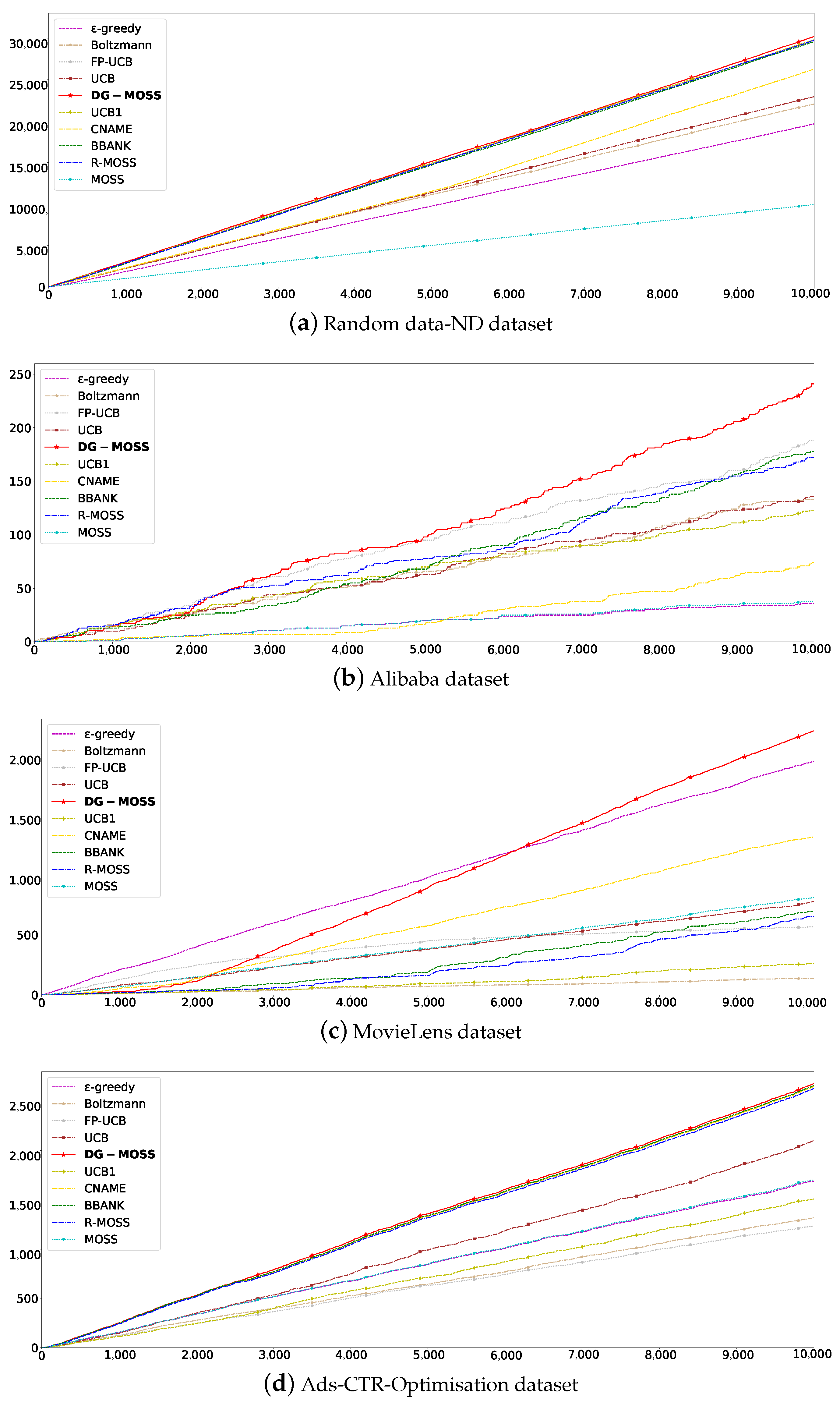
Reinforcement learning is based on the reward hypothesis. All goals can be described by maximizing the expected cumulative rewards. In order to obtain the best behavior in reinforcement learning, we need to maximize the expected cumulative reward. Therefore, the algorithm with a large total reward value can perform the best. Figure 1a–d correspond to Random data-ND, Alibaba, MovieLens, and Ads-CTR-Optimisation datasets, respectively. Figure 1a is a data-dense dataset in which the total reward value of DG-MOSS is slightly higher than that of Boltzmann controlled by random parameters and extended time slots approaching R-MOSS. Figure 1b,c represent sparse datasets with a medium data scale. With the increase in the number of iterations, the total reward value increases steadily and is finally better than all compared algorithms. Figure 1d is a small-sized sparse dataset. In Figure 1a–d,we can observe significant variations in the total rewards among the nine contrasting methods across four distinct datasets. This disparity arises from the distinct scenarios considered by each strategy and the disparate methodologies employed in computing rewards. Particularly in Figure 1b, which entails more intricate shopping data, fluctuations during training may occur due to the complexity of information involved. Regarding Figure 1c, given the heightened subjective nature of music data, DG-MOSS can leverage post-interaction feedback more effectively as training progresses. In the iteration, the total reward value not only maintains linear growth but is also better than other algorithms. Due to the different densities of datasets in different parts, DG-MOSS can adapt to different datasets with sufficiently trained recommendation, particularly when dealing with sparse datasets.

5.2.2. Average Rewards

The average reward is the average of reward values of all rounds, which can better reflect the convergence and stability of the algorithm. Figure 2a–d correspond to Random data-ND, Alibaba, MovieLens, and Ads-CTR-Optimisation datasets, respectively. In Figure 2a, DG-MOSS is better than Boltzmann [18], CNAME [19], UCB1 [3], FP-UCB [23], BBANK [26], and R-MOSS [25], which all perform stably on this dataset, and the average reward is higher than MOSS [24] up to 2. In Figure 2b, the average reward of DG-MOSS is better than CNAME [19], which also has gradually stable performance. In Figure 2c, the average reward of DG-MOSS gradually exceeds $\epsilon$-greedy [20], which performs stably in this dataset. All algorithms are stable, as shown in Figure 2d. For the datasets Figure 2a,b,d, the average reward remains stable, and the value obtained is the maximum. For the dataset Figure 2c, the average reward increases in learning and reaches a stable peak in all algorithms. It is worth noting that, in the initial period, the average reward value of DG-MOSS fluctuates drastically rather than evolving steadily. This may be because initially, a large number of arms does not interact with the reinforcement learning agent, resulting in less stable feedback. In Figure 2, the red line represents DG-MOSS, which performs well on all four datasets after sufficient training due to its ability to not only fully utilize feedback information but also to employ multiple action selection.

5.2.3. Parameter Analysis

There are some algorithms whose parameter sizes and ranges are specified, such as $\epsilon$-greedy [20], Boltzmann [18], and UCB1 [3]. We kept the basic parameters ($Parameters1$) and exploration coefficient parameters ($Parameters2$) of each algorithm consistent to ensure the fairness of the experiment. The basic parameters ($Parameters1$) exist in the original algorithm; some $Parameters2$ exist and some do not. In DG-MOSS, $Parameters1$ are fixed $\sqrt{3}$ in $mis=\sqrt{\frac{3log\left(S\right)}{s}}$, and $Parameters2$ are the exploration probability c. The term $mis$ in the current round signifies the threshold demarcating the total number of arm pulls, denoted as S, and the number of pulls from the current arm, denoted as s. As the exploration probability c undergoes alterations, there are corresponding shifts in both the average reward and average regret. Consequently, for fairness in comparison, the selection of identical parameter values was made. This approach ensures consistency across different exploration probabilities, facilitating a more precise evaluation of outcomes under varied conditions. Here, the exploration probability $c=0.1$ was used. Although random algorithms $\epsilon$-greedy [20], Boltzmann [18] and CNAME [19]; upper bound of confidence algorithms UCB [3] and UCB1 [3]; grouping algorithms FP-UCB [23] and BBANK [26]; and optimal strategy algorithms MOSS [24] and R-MOSS [25] have better performance, DG-MOSS has the maximum average reward and the lowest average regret. This shows the stability of the algorithm.

In the analysis of these parameters, the average rewards and average regrets of DG-MOSS are shown in

Table 1. Description of parameters.

Algorithms	Parameters 1	Parameters 2	Average Rewards	Average Regrets
$\epsilon$-greedy	0.05	NULL	0.1690	0.8310
Boltzmann	1	NULL	0.1318	0.8669
CNAME	$\sqrt{3}$	0.1	0.2648	0.7342
UCB	$\sqrt{3}$	NULL	0.2103	0.7897
UCB1	$\sqrt{2}$	NULL	0.1510	0.8490
FP-UCB	$\sqrt{3}$	0.1	0.1237	0.7562
BBANK	$\sqrt{3}$	0.1	0.2654	0.7346
MOSS	$\sqrt{3}$	NULL	0.1703	0.8297
R-MOSS	$\sqrt{3}$	0.1	0.2631	0.7369
DG-MOSS	$\sqrt{3}$	0.1	0.2681	0.7319

. We used the dynamic grouping to improve reinforcement learning algorithm of MOSS by increasing the exploration coefficient.

According to step 9 of Algorithm 3, it can be inferred that the value of probability parameter $P_1$ is related to the control of action selection. The quantity of dynamically grouped data also plays a significant role, and the varying impacts of different parameters on the final results further indicate the intentional design of probability parameters in DG-MOSS. Here, the selection of exploration parameters is related to K. The K used in this Ads-CTR-Optimisation datasets experiment is 85. We can choose according to the actual situation. Through experimental comparison, we use $\frac{6}{85}$ as the probability parameter $0<P_1<1$. The average rewards of different probability parameters are shown in

Table 2. Probability parameters.

Parameters	Average Rewards
$4/85$	0.2076
$5/85$	0.2673
$6/85$	0.2681
$7/85$	0.2656
$8/85$	0.2659

.

5.2.4. Adaptive $T_i$

In Algorithm 3, we set episode length $T_i=8log\left(\frac{T\ast {\left(T+1\right)}^2}{{\left(avg-mis\right)}^2}\right)$ related to the return value of the agent, which is adaptively proposed. Compared with the initial 1000 in different scenarios, Random data-ND is a dense dataset, Alibaba and Movie are sparse datasets with large scale, and Ads-CTR-Optimisation is a medium-sized sparse dataset. The number of episodes is reduced, as shown in

Table 3. Number of training episodes.

Datasets	Episode
Initial	1000
Random data-ND	24
Alibaba	44
Movie	34
Ads-CTR-Optimisation	638

.

The experimental results show that the episode difference with large-scale and dense datasets can reach more than 956 (1000-44), and the episode difference between medium-scale datasets can also reach more than 362 (1000-638). So, the optimization effect is obvious. Thus, significant improvements are attributed to the combined influence of the total time step T, grouping parameter $mis$, and feedback information $avg$ to jointly affect the episodes, which synergistically complement each other when integrated with the dynamic grouping process in recommendation interactions. There is no need to adjust the parameters manually and adjust the episode in the training automatically.

5.2.5. Robustness

Regardless of the type of user data, such as movies, shopping, or advertising, which has an open nature, some businesses or individuals inject fake data into the recommendation system from the perspective of their own interests, attempting to alter the recommendation results. This is known as a recommendation attack. Common recommendation attacks include random attacks and average attacks. Random attacks involve adding 1%, 3%, 5%, and 10% of random entries to attack. Average attacks involve adding 1%, 3%, 5%, and 10% of entries to attack, with the mean of the dataset being added as one of the entries. Under attack conditions with 1%, 3%, and 5% data, the fluctuations of DG-MOSS remain within a small range. The attack with 10% data is relatively strong and has some impact on all models. Since this study focuses on maximizing rewards for recommendations, the robustness is demonstrated by achieving the maximum reward value even under different attack conditions, which helps in selecting the arms. As shown in

Table 4. Random attacks (R) and average attacks (A) on the movie dataset.

Algorithms	Original	1% R	3% R	5% R	10% R	1% A	3% A	5% A	10% A
$\epsilon$-greedy	0.1944	0.1932	0.2015	0.2070	0.2186	0.1969	0.2131	0.2291	0.2574
Boltzmann	0.0139	0.0192	0.0276	0.0368	0.0546	0.0143	0.0157	0.0181	0.0266
CNAME	0.2296	0.2266	0.1671	0.2496	0.2562	0.2420	0.2347	0.2696	0.2860
UCB	0.0778	0.0815	0.0870	0.0962	0.1092	0.0850	0.1022	0.1179	0.1504
UCB1	0.0262	0.0357	0.0356	0.0415	0.0614	0.0310	0.0406	0.0411	0.0678
FP-UCB	0.0568	0.0421	0.0496	0.0546	0.0706	0.0636	0.0498	0.0547	0.0792
BBANK	0.1983	0.2379	0.2526	0.2562	0.2643	0.2421	0.2441	0.2494	0.2978
MOSS	0.0809	0.0847	0.0908	0.0983	0.1130	0.0887	0.1073	0.1220	0.1541
R-MOSS	0.0653	0.0621	0.0710	0.751	0.0908	0.0667	0.0752	0.0865	0.1430
DG-MOSS	0.2378	0.2396	0.2539	0.2585	0.2720	0.2422	0.2609	0.2729	0.2996

,

Table 5. Random attacks (R) and average attacks (A) on the advertising dataset.

Algorithms	Original	1% R	3% R	5% R	10% R	1% A	3% A	5% A	10% A
$\epsilon$-greedy	0.1690	0.1720	0.1756	0.1846	0.1935	0.1774	0.1896	0.2052	0.2405
Boltzmann	0.1318	0.1332	0.1460	0.1503	0.1568	0.1346	0.1469	0.1587	0.1805
CNAME	0.2648	0.2657	0.2712	0.2725	0.2829	0.2698	0.2841	0.3006	0.3315
UCB	0.2103	0.2088	0.2113	0.2289	0.2312	0.2091	0.2344	0.2409	0.2753
UCB1	0.1510	0.1581	0.1584	0.1681	0.1780	0.1572	0.1695	0.1768	0.220
FP-UCB	0.1237	0.1180	0.1314	0.1400	0.1576	0.1190	0.1340	0.1392	0.1614
BBANK	0.2654	0.2684	0.2711	0.2755	0.2850	0.2745	0.2867	0.3011	0.3317
MOSS	0.1703	0.1736	0.1780	0.1855	0.1987	0.1786	0.1938	0.2082	0.2440
R-MOSS	0.2631	0.2640	0.2678	0.2719	0.2831	0.2704	0.2834	0.2983	0.2766
DG-MOSS	0.2681	0.2693	0.2723	0.2762	0.2853	0.2748	0.2868	0.3013	0.3322

and

Table 6. Random attacks (R) and average attacks (A) on the shopping dataset.

Algorithms	Original	1% R	3% R	5% R	10% R	1% A	3% A	5% A	10% A
$\epsilon$-greedy	0.0036	0.0075	0.0089	0.0076	0.0096	0.0041	0.0037	0.035	0.0040
Boltzmann	0.0133	0.0158	0.0153	0.0155	0.0199	0.0144	0.0151	0.0154	0.0155
CNAME	0.015	0.0156	0.0223	0.0178	0.0176	0.0284	0.0235	0.0252	0.0206
UCB	0.0136	0.0152	0.0195	0.0178	0.0182	0.0154	0.0189	0.0188	0.0196
UCB1	0.0123	0.0148	0.0163	0.0157	0.0173	0.0155	0.0149	0.0158	0.0148
FP-UCB	0.0188	0.0202	0.0235	0.0233	0.0246	0.0214	0.0287	0.0265	0.0265
BBANK	0.0220	0.0241	0.0283	0.0266	0.0265	0.0291	0.0333	0.0343	0.0315
MOSS	0.0038	0.0071	0.0090	0.0078	0.0096	0.0038	0.0038	0.0038	0.0038
R-MOSS	0.0172	0.0145	0.0229	0.0220	0.0243	0.0228	0.0275	0.0239	0.0286
DG-MOSS	0.0223	0.0250	0.0283	0.0268	0.0280	0.0295	0.0339	0.0344	0.0316

. DG-MOSS performs the best under all attack conditions, which indicates that this algorithm has good robustness.

6. Conclusions

For reinforcement learning recommendation for small and medium-sized data scenarios, considering dynamic interactive feedback, this paper presents a novel SMAB algorithm called DG-MOSS that utilizes adaptive episode in training, which is based on improved MOSS by incorporating dynamic grouping from environment feedback information to ensure the balance of exploration and exploitation and maximizing rewards for recommendations. This algorithm can increase the degree of exploration and exploitation according to the dynamic grouping, solving the insufficiency problem and making full use of feedback information. On the one hand, through analysis and proof, this paper gives the upper bound of the regret value of DG-MOSS, which provides strong theoretical support. On the other hand, extensive experiments were undertaken on four datasets (Random data-ND, Alibaba, MovieLens, and Ads-CTR-Optimisation) with total rewards and average rewards. The maximum reward improvement compared to the second-best model reaches 1.02%, while the improvement compared to the worst baseline model can reach up to 36.32%. In summary, DG-MOSS is a stable and robust SMAB algorithm in recommendation. Extensive studies focus on combining deep learning and reinforcement learning to address problems. In the future, we will continue to investigate adaptive approaches based on big data by adding deep learning.

References

- Sutton, R.; Barto, A. Reinforcement learning: An Introduction. Robotica 1999, 17, 229–235. [Google Scholar] [CrossRef]
- Silver, D.; Singh, S.; Precup, D. Reward is enough. Artif. Intell. 2021, 299, 103535. [Google Scholar] [CrossRef]
- Auer, P. Finite-time analysis of the multiarmed bandit problem. Robotica 2002, 47, 235–256. [Google Scholar]
- Gutowski, N.; Amghar, T.; Camp, O. Gorthaur: A portfolio approach for dynamic selection of multi-armed bandit algorithms for recommendation. In Proceedings of the 31th International Conference on Tools with Artificial Intelligence (ICTAI), Portland, OR, USA, 4–6 November 2019; pp. 1164–1171. [Google Scholar]
- Tong, X.; Wang, P.; Niu, S. Reinforcement learning-based denoising network for sequential recommendation. Appl. Intell. 2023, 53, 1324–1335. [Google Scholar] [CrossRef]
- Qin, J.; Wei, Q.; Zhou, B. Research on optimal selection strategy of search engine keywords based on multi-armed bandit. In Proceedings of the 49th Hawaii International Conference on System Sciences (HICSS), Koloa, HI, USA, 5–8 January 2016; pp. 726–734. [Google Scholar]
- Takeuchi, S.; Hasegawa, M.; Kanno, K. Dynamic channel selection in wireless communications via a multi-armed bandit algorithm using laser chaos time series. Sci. Rep. 2020, 10, 1574. [Google Scholar] [CrossRef]
- Angulo, C.; Falomir, Z.; Anguita, D. Bridging cognitive models and recommender systems. Cogn. Comput. 2020, 12, 426–427. [Google Scholar] [CrossRef]
- Li, Y.; Wang, S.; Pan, Q. Learning binary codes with neural collaborative filtering for efficient recommendation systems. Knowl. Based Syst. 2019, 172, 64–75. [Google Scholar] [CrossRef]
- Dhelim, S.; Aung, N.; Bouras, M.A. A survey on personality-aware recommendation systems. Artif. Intell. Rev. 2022, 55, 2409–2454. [Google Scholar] [CrossRef]
- Yang, Y.; Chen, C.; Lu, T. Hierarchical reinforcement learning for conversational recommendation with knowledge graph reasoning and heterogeneous questions. IEEE Trans. Serv. Comput. 2023, 16, 3439–3452. [Google Scholar] [CrossRef]
- Pang, G.; Wang, X.; Wang, L.; Hao, F.; Lin, Y.; Wan, P.; Min, G. Efficient Deep Reinforcement Learning-Enabled Recommendation. IEEE Trans. Sci. Eng. 2023, 10, 871–886. [Google Scholar] [CrossRef]
- Gu, H.; Xia, Y.; Xie, H.; Shi, X.; Shang, M. Robust and efficient algorithms for conversational contextual bandit. Inf. Sci. 2024, 657, 119993. [Google Scholar] [CrossRef]
- Kanade, V.; Liu, Z.; Kanade, V. Distributed non-stochastic experts. Adv. Neural Inf. Process. Syst. 2012, 25, 260–268. [Google Scholar]
- Agrawal, P.; Tulabandula, T. Learning by repetition: Stochastic multi-armed bandits under priming effect. In Proceedings of the 36th International Conference on Uncertainty in Artificial Intelligence (UAI), Online, 3–6 August 2020; pp. 470–479. [Google Scholar]
- Gopalan, P.; Hofman, J.M.; Blei, D.M. Scalable recommendation with hierarchical poisson factorization. In Proceedings of the 31th International Conference on Uncertainty in Artificial Intelligence (UAI), Amsterdam, The Netherlands, 12–16 July 2015; pp. 326–335. [Google Scholar]
- Wang, L.; Bai, Y.; Sun, W. Fairness of exposure in stochastic bandits. In Proceedings of the 38th International Conference on Machine Learning (ICML), Online, 18–24 July 2021; pp. 7700–7709. [Google Scholar]
- Guo, X.; Song, J.; Fang, Y. Explain in Simple Terms Reinforcement Learning; Publishing House of Electronics Industry: Beijing, China, 2020. [Google Scholar]
- Zhang, X.; Zou, Q.; Liang, B. An adaptive algorithm in multi-armed bandit problem. Comput. Res. Dev. 2019, 56, 643–654. [Google Scholar]
- Green, L.; Fry, A.; Myerson, J. Discounting of delayed rewards: A life-span comparison. Psychol. Sci. 1994, 5, 33–36. [Google Scholar] [CrossRef]
- Hong, X.; Qiao, T.; Qingsheng, Z. A multiplier bootstrap approach to designing robust algorithms for contextual bandits. IEEE Trans. Neural Netw. Learn. Syst. 2022, 34, 9887–9899. [Google Scholar]
- Wang, T.; Shi, X.; Shang, M. Diversity-Aware Top-N Recommendation: A Deep Reinforcement Learning Way. In Proceedings of the 8th CCF International Conference on Big Data (CCF BigData), Chongqing, China, 22–24 October 2020; pp. 1324–1335. [Google Scholar]
- Panaganti, K.; Kalathil, D.M. Bounded regret for finitely parameterized multi-armed bandits. IEEE Control Syst. Lett. 2021, 5, 1073–1078. [Google Scholar] [CrossRef]
- Audibert, J.; Bubeck, S. Minimax policies for adversarial and stochastic bandits. In Proceedings of the 22nd International Conference on Learning Theory (COLT), Montreal, QC, Canada, 18–21 June 2009; pp. 217–226. [Google Scholar]
- Wei, L.; Srivastava, V. Nonstationary stochastic multiarmed bandits: Ucb policies and minimax regret. arXiv 2021, arXiv:2101.08980. [Google Scholar]
- Karpov, N.; Zhang, Q. Batched coarse ranking in multi-armed bandits. In Proceedings of the 34th International Conference on Neural Information Processing Systems (HeurIPS), Online, 6–12 December 2020; pp. 16037–16047. [Google Scholar]
- Esfandiari, H.; Karbasi, A.; Mehrabian, A.; Mirrokni, V. Regret bounds for batched bandits. In Proceedings of the 35th International AAAI Conference on Artifical Intelligence (AAAI), Online, 2–9 February 2021; pp. 7340–7348. [Google Scholar]
- Sun, D. Wald’s identity and geometric expectation. Am. Math. Mon. 2020, 127, 716. [Google Scholar] [CrossRef]
- Hoeffding, W. Probability inequalities for sums of bounded random variables. Am. Stat. Assoc. 1963, 58, 13–30. [Google Scholar] [CrossRef]
Figure 1.
Total rewards. (a–d) The X axis represents the value of total rewards, and the Y axis represents the training epochs.
Figure 2.
Average rewards. (a–d) The X axis represents the value of total rewards, and the Y axis represents the training epochs.