Stability Analysis in Multi-VSC (Voltage Source Converter) Systems of Wind Turbines

Abstract

In this paper, a holistic nonlinear state-space model of a system with multiple converters is developed, where the converters correspond to the wind turbines in a wind farm and are equipped with grid-following control. A novel generalized methodology is developed, based on the number of the system’s converters, to compute the equilibrium points around which the model is linearized. This is a more solid approach compared with selecting operating points for linearizing the model or utilizing EMT simulation tools to estimate the system’s steady state. The dynamics of both the inner and outer control loops of the power converters are included, as well as the dynamics of the electrical elements of the system and the digital time delay, in order to study the dynamic issues in both high- and low-frequency ranges. The system’s stability is assessed through an eigenvalue-based stability analysis. A participation factor analysis is also used to give an insight into the interactions caused by the control topology of the converters. Time domain simulations and the corresponding frequency analysis are performed in order to validate the model for all the control interactions under study.

1. Introduction

In recent decades, the wind energy sector has experienced significant growth. According to the latest Renewables Global Status Report by REN21, global wind power capacity increased by more than 77 GW in 2022. This includes 68.4 GW of onshore and approximately 8.8 GW of offshore installations, marking a 9% rise in the total operational capacity to an estimate of 906 GW [1]. The Global Wind Energy Council (GWEC) forecasts an addition of 680 GW to the global wind capacity from 2023 to 2027, including 130 GW offshore. By the end of 2030, wind energy is anticipated to reach a landmark 2 TW of installed capacity [2].

The high increase in wind-power penetration has made the power system more efficient and flexible, mainly because it is coming to be dominated by high-power electronic Voltage Source Converters (VSC) [3,4]. On the other hand, many challenges for the power system’s stability and synchronization to the grid have been arising, as the number of components connected to the system is being increased [5]. Therefore, extensive research has been conducted in the area of dynamic interactions between the grid-connected converters of wind turbines on wind farms.

The small-signal stability of a converter-based system is the system’s ability to overcome a small disturbance and return to a steady state [6]. The main small-signal stability analysis methods for converter-based systems are impedance-based analysis—which is mainly preferred in “black-box” systems—and eigenvalue analysis [7]. In impedance-based analysis, the system’s equivalent impedances seen from the Point of Common Coupling (PCC) are used in order to represent the small-signal dynamics between the converter control system and the grid [8]. The Nyquist stability criterion evaluates the system’s stability based on the system’s open-loop gain [7]. In eigenvalue analysis, the state-space model of the whole system is formulated, providing a deep input into the system and control dynamics. Linearization of the nonlinear model is applied at the obtained equilibrium points that correspond to the model’s state variables, and then the system’s eigenvalues are obtained by implementing a modal analysis. The formulated eigenvalue plots depict the system’s stability [9].

State-space modeling is chosen for conducting sensitivity analysis and gaining insights into the internal states of the system, which can subsequently be assessed for stability using eigenvalue analysis. Research on various state-space modeling methods for converter-based systems is well-documented in [10,11,12,13]. These studies emphasize enhanced modularity and offer detailed descriptions of the dynamic states prevalent in wind turbine systems. However, they lack a methodology for computing the equilibrium points around which the model is linearized, as they either set them directly equal to chosen operating points or they rely on ElectroMagnetic Transients (EMTs) simulations tools for obtaining them through power flow analysis. In [14,15], a Component Connection Method (CCM) was utilized, where the system was decomposed into multiple components and a linear algebra matrix was formed based on the interconnections of the components; the state-space model of the system was obtained by combining the state-space submodels of the components using the linear algebra matrix. However, it was difficult to represent the internal connections caused by the control couplings of the model [16]. A methodology for computing the equilibrium points was also not provided, and chosen operating points were instead used for the model’s linearization.

In [17], a detailed modular methodology was used to derive the linearized state-space model after computing the equilibrium points; however, it was limited to only using an L filter, without a capacitor in the filter, and this constitutes the dynamic situation of the model, which is much simpler than is the case with LC or LCL filters. The case of the LC filter was studied in [18] in detail; the limitation was that the equilibrium points’ computation was based on a single-VSC system and could not be utilized in a system with multiple VSCs. Time delay was also not considered in either of the studies [17,18], so the dynamics of the high frequency phenomena could not be analyzed. Systems with multiple VSCs have been studied in [19,20,21] too; however, these studies mainly focused on the Phase-Locked Loop (PLL)’s dynamic impact, and the outer-loop control was overlooked.

In this paper, therefore, the internal interactions of a nonlinear state-space model of a power system with multiple grid-connected VSCs were studied, covering the abovementioned research gaps. For that purpose, the model entailed an LC filter and outer-loop control, and the VSC sub-models corresponded to the wind turbines of a wind farm. A novel generalized methodology, based on the number of VSCs in the system, was utilized in order to estimate the equilibrium points of each state variable of the nonlinear model; thus, the model could be linearized around them for several system and control parameters. The dynamics within the wind farm were then highlighted, first by applying the eigenvalue-based stability analysis and then the controller gains were swept for each converter. In this way, the equilibrium points of the whole model were recalculated and led to another equilibrium state and its corresponding eigenvalue analysis. Hence, the interactions of both the inner and outer control loops were identified by observing the eigenvalues trace for each controller, as well as by implementing participation factor analysis for the critically unstable system modes. Simulation results in the time domain and the frequency domain were carried out in order to validate the eigenvalue-based stability analysis results.

2. State-Space Model of a System with n Voltage Source Converters

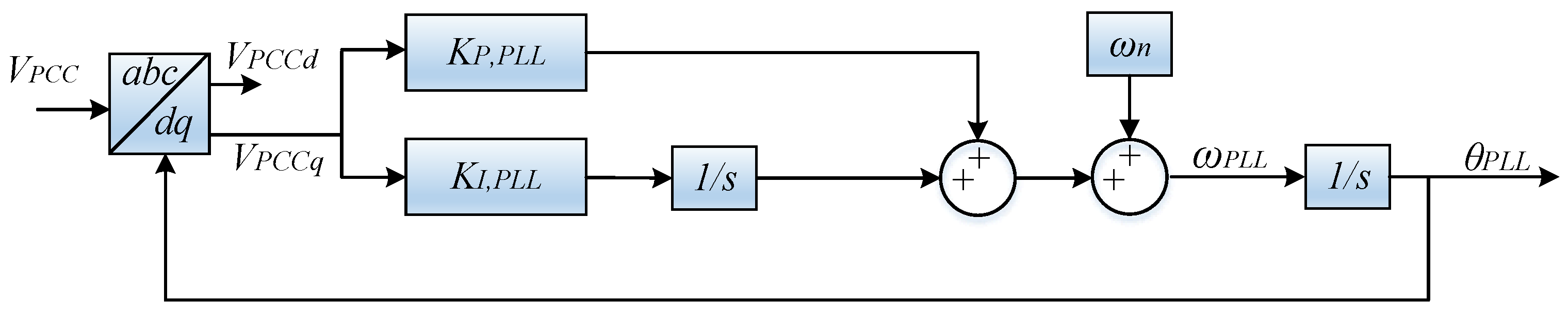
The focus of this study was on the grid-side converters of wind turbines in a wind farm and their potential dynamic interactions with the grid. The control architecture of a grid-connected single-converter system is depicted in Figure 1. This system incorporates a grid-following converter that utilizes vector Current Control (CC). The concept is derived from [22]; it employs a PLL to synchronize the converter with the grid, assuming a consistent DC link voltage at the inverter. The regulation of active power adheres to a specified reference value using open-loop control, which is considered adequate under the assumption of an ideal converter. The input feed-forward voltage into the CC loop, which is the voltage at PCC $V_{PCC}$, integrates a low-pass filter in the d-q domain (FF, LPF in Figure 1). An Alternating-Voltage magnitude Controller (AVC), which includes a low-pass filter (AVC, LPF in Figure 1), is also utilized to regulate the voltage fed at the PLL of each VSC, based on the study in [23]. The AVC is of high importance in order to ensure the system’s normal operation, especially in weak-grid cases. The control topologies of the PLL, the current controller and the AVC are shown in Figure 2, Figure 3 and Figure 4, respectively.

The assumption utilized for deriving the initial state-space model of the multi-converter system is that all VSCs have homogeneous dynamics; meaning, their topology and control philosophy are all the same. In the configuration of the parallel connection of n such converters the converters share a common point of synchronization as well as a common PCC; therefore, the transformer’s leakage inductance of each VSC was not considered in this work, in order to simplify the complexity of the final model, which is shown in Figure 5.

A state-space model for a single-wind-turbine system has been formulated, as detailed in [23], to characterize small-signal instabilities. This model is outlined in (1) and features nonlinear state equations that capture the system’s control dynamics. Each component of the system is represented by these equations, and the complete nonlinear state-space model arises from the combination of the individual state-space models of each system component.

$$\begin{array}{cc}\hfill & \dot{x}=Ax+R(x,u)\hfill \\ \hfill & y=S(x,u)\hfill \end{array}$$

(1)

where $R(x,u)$ describes the non-linear dependencies in the model. The state equations describing the small-signal model of the single-VSC system in Figure 1 are presented in Appendix A.

The abovementioned nonlinear model of one VSC can be used to compose a system with n parallel VSCs corresponding to n wind turbines on a wind farm. The state equations of each grid-connected converter are combined in order to form the total state-space model of the system with n VSCs. The holistic nonlinear state-space model is given in (2):

$$\begin{array}{cc}\hfill \left[\begin{array}{c}{\dot{x}}_{VSC1}\\ {\dot{x}}_{VSC2}\\ ⋮\\ {\dot{x}}_{VSCn}\end{array}\right]& =\left[\begin{array}{cccc}{A}_{VSC1}& 0& \cdots & 0\\ 0& A_{VSC2}& \ddots & ⋮\\ ⋮& & \ddots & 0\\ 0& \cdots & 0& A_{VSCn}\end{array}\right]\left[\begin{array}{c}{x}_{VSC1}\\ x_{VSC2}\\ ⋮\\ x_{VSCn}\end{array}\right]\hfill \\ \hfill & +\left[\begin{array}{cccc}{R}_{VSC1}& 0& \cdots & 0\\ 0& R_{VSC2}& \ddots & ⋮\\ ⋮& & \ddots & 0\\ 0& \cdots & 0& R_{VSCn}\end{array}\right]\left[\begin{array}{c}{x}_{VSC1},u_{VSC1}\\ x_{VSC2},u_{VSC2}\\ ⋮\\ x_{VSCn},u_{VSCn}\end{array}\right]\hfill \end{array}$$

(2)

The system parameters of the system in Figure 1 and the control parameters of the corresponding state-space model in Appendix A are listed in

Table 1. System and Default Control Parameters of the System in Figure 1.

	Description	Value
VS	Grid Phase Voltage	311 V
fn	Rated Grid Frequency	50 Hz
VDC	DC Link Voltage Reference	800 V
LF	Filter Inductance	5 mH
RF	Filter Resistance	0.1 $\Omega$
CF	Filter Capacitance	10 $\mathsf{\mu }$F
fsw	Switching Frequency	20 kHz
fS	Sampling Frequency	20 kHz
VPCCref	Reference PCC Voltage	280 V
Pref	Nominal Active Power	30 kW
ωFF,LPF	Cutoff frequency of FF Voltage	100 rad/s
ωAVC,LPF	Cutoff frequency of AVC	50 rad/s
KI,CC0	Default Integral Gain of Current Control	666.7
KP,CC0	Default Proportional Gain of Current Control	33.3
KI,PLL0	Default Integral Gain of PLL	0
KP,PLL0	Default Proportional Gain of PLL	0.1637
KI,a0	Default Integral Gain of AVC	10
KP,a0	Default Proportional Gain of AVC	0

.

3. Equilibrium Points Computation and Eigenvalue Analysis in a Multi-VSC System

First, two dq frames need to be defined in order to describe the dynamics related to the PLL. These are the grid dq frame and the control dq frame, both of which have been analytically introduced in [23]. The converter current $I_L$ and the PCC voltage $V_{PCC}$ are the variables impacted by the control dq frame. The resulting equations from the linearization between the two dq frames, which express the transformation between the grid and the control dq frame, are shown below (variables in the control dq frame are indicated by the superscript c):

$$\Delta V_{PCCd}^c=\Delta V_{PCCd}+V_{PCCq,0}\Delta \theta$$

(3)

$$\Delta V_{PCCq}^c=\Delta V_{PCCq}-V_{PCCd,0}\Delta \theta$$

(4)

$$\Delta I_{Ld}^c=\Delta I_{Ld}+I_{Lq,0}\Delta \theta$$

(5)

$$\Delta I_{Lq}^c=\Delta I_{Lq}-I_{Ld,0}\Delta \theta$$

(6)

where $\Delta \theta$ is the phase shift between the two dq frames.

To evaluate the stability of the converter-based system, the potential equilibrium points need to be identified first through the linearized state-space model. Assessing the system’s local stability involves using a linear approximation of this state-space model, represented as

$$\dot{x}=Ax$$

(7)

In this context, the matrix A, known as the Jacobian matrix, comprises partial derivatives relating to the system at steady operating points. These equilibrium points are established by setting the state equations of the system to $\dot{x}=0$ and solving for them.

In Section 3.1, a generalized methodology is analytically described for obtaining the system’s equilibrium points based on the number of VSCs connected to the PCC.

3.1. Methodology for Equilibrium Points Computation

The equilibrium states for each converter consist of the common voltage at the PCC, $V_{PCC,0}$, and the inductor current $I_{Li,0}$—both in the dq reference frame and as already used in (3)–(6)—where $i=1\dots n$ and corresponds to the converter under study, $VS{C}_i$. The equilibrium states of the wind farm’s output current $I_{o,0}$ should also be estimated, as this is a state variable that is utilized in the grid impedance submodel of each VSC.

When $V_{PCCq}$ is maintained at zero by the PLL its corresponding equilibrium state, denoted as $V_{PCCq,0}$, also equals zero. In line with this and following the definition of $V_M$ as detailed in [23] it follows that $V_{PCCd,0}$ is equivalent to $V_{PCCref}$. Similarly, the equilibrium state of the d-axis inductor current, $I_{Ldi,0}$, matches $I_{Ldref}$. The equilibrium state for the q-axis inductor current, $I_{Lqi,0}$, is deduced by applying Kirchoff’s Voltage Law (KVL) to the grid side:

$$V_{PCCd,0}=V_{Sd,0}+R_S{I}_{od,0}-{\omega }_n{L}_S{I}_{oq,0}$$

(8)

The correlation between each converter’s inductor current and the total system’s output current along the d- and q-axes is characterized as follows:

$$I_{od,0}=n{I}_{Ldi,0}=n{I}_{Ldref}$$

(9)

$$I_{oq,0}=\left(\frac{K_{I,a1}+...+K_{I,an}}{K_{I,ai}}\right)I_{Lqi,0}-n{\omega }_n{V}_{PCCd,0}{C}_{Fi}$$

(10)

where n is the number of VSCs corresponding to the wind turbines.

The d-axis grid voltage, represented as $V_{Sd,0}$, is determined by the following formula:

$$V_{Sd,0}=\left|V_{Sabc}\right|cos\delta$$

(11)

in which $\delta$ symbolizes the grid angle relative to each converter’s capacitor voltage. This angle can be estimated by considering the active power each converter injects into the grid in the abc frame.

$$P_i=\frac{3}{2}\frac{|V_{PCCabc}\left|\right|V_{Sabc}|sin\left(\delta \right)}{{\omega }_n{L}_S}$$

(12)

As previously noted, the control strategy is focused on the d-axis, which means the active power in the dq frame is computed using only the d-axis variables:

$$P_i=\frac{3}{2}{V}_{PCCd}{I}_{od}=\frac{3}{2}\left|V_{PCCabc}\right|I_{od}$$

(13)

Consequently, the angle $\delta$ can be estimated through (12) and (13), leading to the following formula:

$$cos\delta =\sqrt{1-{\left(\frac{{\omega }_n{L}_S{I}_{od}}{|V_{Sabc}|}\right)}^2}$$

(14)

By incorporating (9), (10), (11) and (14) into (8), we can derive the equilibrium state of the inductor current for each VSC on the q-axis as shown in (15):

$$\begin{array}{c}\hfill I_{Lqi,0}=\left(\frac{K_{I,ai}}{K_{I,a1}+\dots +K_{I,an}}\right)\times \\ \hfill \frac{\sqrt{|V_{Sabc}{|}^2-{\left(n{\omega }_n{L}_S{I}_{Ldref}\right)}^2}+n{R}_S{I}_{Ldref}-V_{PCCref}\left(1-n{\left({\omega }_n\right)}^2{L}_S{C}_{Fi}\right)}{{\omega }_n{L}_S}\end{array}$$

(15)

These equilibrium points are estimated for all the VSCs that are connected to the grid; in that way, a holistic nonlinear model can be linearized around them.

3.2. Eigenvalue Analysis

The grid strength is defined by the Short Circuit Ratio (SCR), which is the ratio of the short circuit power by all VSCs at PCC $S_{SC}$ and the rated power of the inverter $S_N$. The SCR is given by

$$SCR=\frac{S_{SC}}{S_N}=\frac{\frac{3}{2}\frac{{\left(V_S\right)}^2}{|Z_S|}}{\frac{3}{2}n{V}_{PCC}{I}_{Ldref}}$$

(16)

Hence, the strength of the grid is influenced by its impedance, with an increase in impedance resulting in a reduction in the short circuit power. Also, the more converters that are connected to the system, with the same grid impedance, the higher the total rated inverter power becomes and the grid becomes weaker.

In this study, a scenario with a weak grid and an SCR of 1.5 was examined. The eigenvalue analysis of the small-signal model was conducted using the control parameters specified in Table 1. The bandwidth of the current controller was set to 1 kHz, targeting a closed-loop current regulation at 1/20 of the switching frequency; the standard bandwidth for the PLL is $7.27$ Hz. The grid inductance $L_S$ was obtained by (16), and the grid resistance $R_S$ was assumed to be zero.

An eigenvalue sensitivity analysis was performed to assess the small-signal stability and the interactions influenced by the controllers across both low- and high-frequency ranges. This analysis adjusted the control parameters of the system’s control structures to pinpoint the levels associated with instability. The equilibrium states of the integrated state-space model were recalculated with each adjustment of the tested controller until instability was caused. Instability is detected when the real part of a complex eigenvalue becomes positive, indicating negative damping. Consequently, a new eigenvalue analysis was conducted each time a parameter was adjusted, ultimately producing an eigenvalue trace that illustrated the stability trend of the tested control parameter. This method is illustrated in Figure 6.

At first, the proportional gain of the current controller for a single VSC K_P,CC1 was swept from 0.1 (deep blue) to 10 (deep red) times its standard value K_P,CC0. The resulting eigenvalues indicating instability are displayed in Figure 7, highlighting the critical gain and frequency. As the proportional gain of the current controller increased, the system tended toward instability, with the critical frequency approximately equal to 1/6 of the sampling frequency $f_S$.

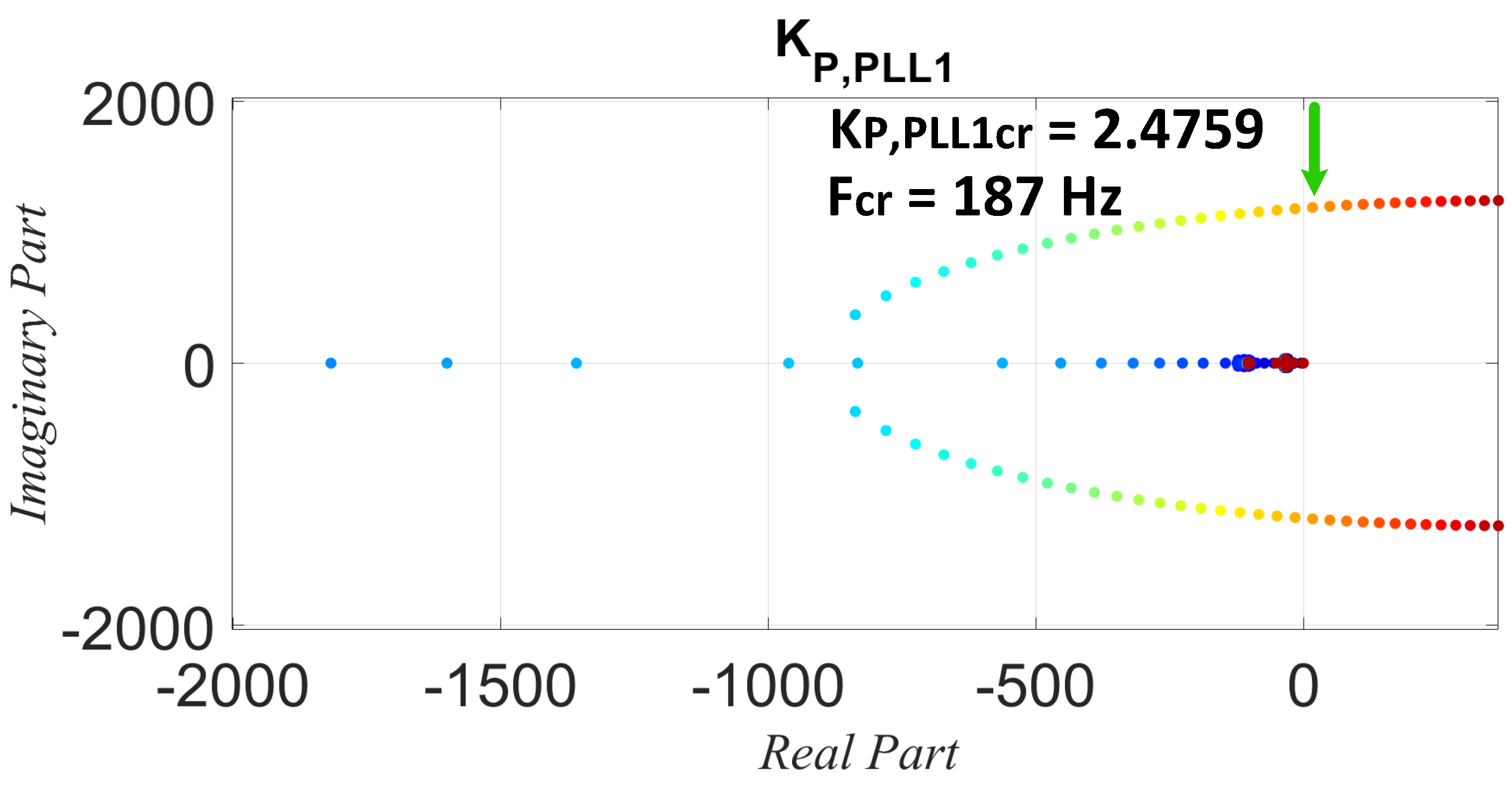
Subsequently, low-frequency interactions were analyzed by varying the PLL proportional gain $K_{P,PLL1}$ of a single VSC in the system from 0.1 (deep blue) to 20 (deep red) times the default value $K_{P,PLL0}$. In that way, the critical PLL bandwidth for instability was determined. The findings, shown in Figure 8, indicate that instability occurred when the PLL proportional gain reached approximately $2.4759$, corresponding to a critical PLL bandwidth of about $110.07$ Hz.

The outer loop of the AVC was also leading to instability in the low-frequency range. This is depicted in Figure 9, where the integral gain $K_{I,a1}$ is varied from 0.1 (deep blue) to 200 (deep red) times the default value $K_{I,a0}$. The eigenvalue analysis shows that the critical case of instability was when $K_{I,acr}=857$ with a dominant frequency close to the 1st harmonic ($f_{cr}=45$ Hz).

4. Participation Factor Analysis and Dynamic Interaction

A participation factor analysis is a useful method for measuring the level of participation of the different state variables in the system’s eigenvalues, and it is conducted to evaluate the sensitivity of controllers in a multi-VSC system having two VSCs (n = 2) placed in parallel. This analysis is vital for identifying the dynamic states that most significantly influence the instability of identified eigenvalue modes. The participation factors are normalized to sum up to 1 in each scenario.

In this context, dynamic states with the index “1” corresponded to $VS{C}_1$, and dynamic states with the index “2” corresponded to $VS{C}_2$. Initially, the analysis focused on how changes in the current controller’s gain $K_{P,CC1}$ of $VS{C}_1$ influenced the system mode’s instability. The results in Figure 10 indicate that the dynamic states of time delay $x_{del,1d},1$ and d-axis current $I_{Ld},1$ in the $VS{C}_1$ were the most critical, particularly the time delay within the current controller’s loop, which was identified as a primary instability factor following the controller design changes.

Furthermore, the analysis was extended to the mode affected by variations in the PLL’s gain $K_{P,PLL1}$ in $VS{C}_1$. The results shown in Figure 11 reveal that the dynamic states of the PLL’s output angle ${\theta }_{PLL},1$ and the q-axis voltage at PCC $V_{PCCq},1$ significantly influenced the mode’s stability. However, the dynamic state of the q-axis output current $I_{oq},2$ in the $VS{C}_2$’s control system had the most pronounced effect. This finding suggests that the instability arose from interactions between the two VSCs’ control systems, especially when changes in one VSC’s PLL bandwidth impacted synchronization with the grid.

Lastly, when examining the mode affected by changes in the AVC’s integral gain $K_{I,a1}$ in $VS{C}_1$, the results in Figure 12 show that the AVC controller’s dynamic states $q_{errac},1$ and $V_{M,LPF},1$ in $VS{C}_1$ predominantly affected the mode’s stability. This case emphasizes the crucial role of $VS{C}_1$’s AVC controller in the system mode stability.

5. Simulation Results

Time domain simulations were carried out by using MATLAB Simulink R2020b and PLECS Blockset in order to validate the eigenvalue-based stability analysis results from Section 3. They were accompanied by the corresponding Fast Fourier Transformation (FFT) analysis, through which we ensured that the dominant frequency in the instant the system tended to become unstable was the same as the critical frequency of instability in the eigenvalue analysis.

A weak-grid-case scenario, with an SCR equal to 1.5, was chosen in order to highlight the dynamic interactions in one of the system’s converters. A system, as shown in Figure 5, with two VSCs $(n=2)$ was simulated in the time domain. A small step change was applied to the control gain of the tested controller in order to identify cases where instability occurred, and the FFT analysis was performed at the beginning of the instability in all the test cases.

A step change was first applied to the proportional gain of the current controller $K_{P,CC1}$ in $VS{C}_1$ in order to show the instability. The system became unstable when this step change resulted in a critical proportional gain value equal to $K_{P,CC1cr}=99.9$; the corresponding dominant frequency of the unstable case was equal to 3.34 kHz. Figure 13a and Figure 14a show the inductor current in $I_{L1}$ in $VS{C}_1$ and highlight this instability case both in the time and frequency domains.

Then, the lower resonances, which were caused by the PLL and the AVC in $VS{C}_1$, were simulated. The PLL proportional gain $K_{P,PLL1}$ was increased in order to identify the bandwidth in which the system was leading to instability; the critical value $K_{P,PLL1cr}$ was equal to $2.55$ where the PLL’s bandwidth was equal to $113.37$ Hz, and the corresponding dominant frequency that led to instability was equal to 182 Hz. These results are shown in Figure 13b and Figure 14b. The same procedure was applied to the AVC in $VS{C}_1$, where a ramp change was applied to its integral controller $K_{I,a1}$; the reason was that a ramp indicates a very large number of steps and would be much more accurate to be used for an integrated value than a single step. The critical value of instability was approximately $K_{I,a1cr}=750$ with a corresponding frequency equal to 44 Hz. These results are shown in Figure 13c and Figure 14c.

The aforementioned results are very close to the corresponding results in Section 3, where the eigenvalue-based stability analysis of the small-signal model with n VSCs was presented; all the results are gathered in

Table 2. Critical control gain and oscillation frequency in eigenvalue-based stability analysis and time domain analysis for a multi-VSC grid-connected system with $n=2$ VSCs.

	Eigenvalue-Based Analysis	Time Domain Analysis
Current Controller	KP,CC1cr = 104.2	KP,CC1cr = 99.9
	Fcr = 3.34 kHz	Fcr = 3.34 kHz
PLL	KP,PLL1cr = 2.4759	KP,PLL1cr = 2.55
	Fcr = 187 Hz	Fcr = 182 Hz
AVC	KI,a1cr = 857	KI,a1cr = 750
	Fcr = 45 Hz	Fcr = 44 Hz

. Therefore, the developed state-space model of the multi-VSC system can describe the interactions introduced by each control loop with very high accuracy.

6. Conclusions

In this paper, a modular nonlinear state-space model of a multi-VSC power system was developed, where one VSC corresponded to a wind turbine of a wind farm. The VSCs were connected to the grid through an LC Filter, and state-space submodels in the dq reference frame for the PLL, the CC and the AVC as well as the digital time delay were developed. The novel methodology used for obtaining the equilibrium points was generalized and based on the number of VSCs, as the obtained formulas of the steady-state currents could be used for several cases of different control and system parameters, and their accuracies were proven by the time domain results in the steady state. The eigenvalue analysis with the eigenvalue traces, as well as the participation factor analysis, showed the impact of each VSC’s controller in the system’s stability in the high- and low-frequency range. The time domain simulations, as well as the FFT analysis when the system started to become unstable, provided results very close to the corresponding eigenvalue-based stability analysis. Therefore, the developed state-space model can be used as a holistic tool that describes quite accurately the small-signal interactions on the grid side of a system with multiple wind turbines and for different control and system parameters.

References

- Bada, J.; Vidal, A.D.; Komazawa, Y.; Ledanois, N.; Yaqoob, H.; Brown, A.; Sawin, J.L.; Abdelnabi, H.; Couzin, H.; El Guindy, A.; et al. Renewables 2023 Global Status Report; Report REN21.2023; REN21 Secretariat: Paris, France, 2023. [Google Scholar]
- GWEC. Global Wind Report 2023; Global Wind Energy Council: Brussels, Belgium, 2023. [Google Scholar]
- Teodorescu, R.; Liserre, M.; Rodríguez, P. Grid Converters for Photovoltaic and Wind Power Systems, 1st ed.; John Wiley & Sons: Hoboken, NJ, USA, 2011. [Google Scholar]
- Kroposki, B.; Johnson, B.; Zhang, Y.; Gevorgian, V.; Denholm, P.; Hodge, B.-M.; Hannegan, B. Achieving a 100% renewable grid: Operating electric power systems with extremely high levels of variable renewable energy. IEEE Power Energy Mag. 2017, 15, 61–73. [Google Scholar] [CrossRef]
- Wen, B.; Boroyevich, D.; Burgos, R.; Mattavelli, P.; Shen, Z. Analysis of D-Q Small-Signal Impedance of Grid-Tied Inverters. IEEE Trans. Power Electron. 2016, 31, 675–687. [Google Scholar] [CrossRef]
- Coelho, E.A.A.; Cortizo, P.C.; Garcia, P.F.D. Small-Signal Stability for Parallel-Connected Inverters in Stand-Alone AC Supply Systems. IEEE Trans. Ind. Appl. 2002, 38, 533–542. [Google Scholar] [CrossRef]
- Amin, M.; Molinas, M. Small-Signal Stability Assessment of Power Electronics Based Power Systems: A Discussion of Impedance- and Eigenvalue-Based Methods. IEEE Trans. Ind. Appl. 2017, 53, 5014–5030. [Google Scholar] [CrossRef]
- Vieto, I.; Sun, J. Small-Signal Impedance Modelling of Type-III Wind Turbine. In Proceedings of the 2015 IEEE Power Energy Society General Meeting, Denver, CO, USA, 26–30 July 2015; pp. 1–5. [Google Scholar]
- Huang, H.; Mao, C.; Lu, J.; Wang, D. Small-signal modelling and analysis of wind turbine with direct drive permanent magnet synchronous generator connected to power grid. IET Renew. Power Gener. 2012, 6, 48–58. [Google Scholar] [CrossRef]
- Kroutikova, N.; Hernandez-Aramburo, C.A.; Green, T.C. State-space model of grid-connected inverters under current control mode. IET Electr. Power Appl. 2007, 1, 329. [Google Scholar] [CrossRef]
- Gontijo, G.F.; Bakhshizadeh, M.K.; Kocewiak, Ł.H.; Teodorescu, R. State Space Modeling of an Offshore Wind Power Plant with an MMC-HVDC Connection for an Eigenvalue-Based Stability Analysis. IEEE Access 2022, 10, 82844–82869. [Google Scholar] [CrossRef]
- Amin, M.; Suul, J.A.; D’Arco, S.; Tedeschi, E.; Molinas, M. Impact of state-space modelling fidelity on the small-signal dynamics of VSC-HVDC systems. In Proceedings of the 11th IET International Conference on AC and DC Power Transmission, Birmingham, UK, 10–12 February 2015; pp. 1–11. [Google Scholar]
- Zhou, J.Z.; Ding, H.; Fan, S.; Zhang, Y.; Gole, A.M. Impact of Short-Circuit Ratio and Phase-Locked-Loop Parameters on the Small-Signal Behavior of a VSC-HVDC Converter. IEEE Trans. Power Deliv. 2014, 29, 2287–2296. [Google Scholar] [CrossRef]
- Wang, Y.; Wang, X.; Chen, Z.; Blaabjerg, F. Small-Signal Stability Analysis of Inverter-Fed Power Systems Using Component Connection Method. IEEE Trans. Smart Grid 2018, 9, 5301–5310. [Google Scholar] [CrossRef]
- Mandrile, F.; Musumeci, S.; Carpaneto, E.; Bojoi, R.; Dragicevic, T.; Blaabjerg, F. State-space modeling techniques of emerging grid-connected converters. Energies 2020, 13, 4824. [Google Scholar] [CrossRef]
- Yang, D.; Wang, X. Unified Modular State-Space Modeling of Grid-Connected Voltage-Source Converters. IEEE Trans. Power Electron. 2020, 35, 9700–9715. [Google Scholar] [CrossRef]
- Cecati, F.; Zhu, R.; Liserre, M.; Wang, X. Nonlinear Modular State-Space Modeling of Power-Electronics-Based Power Systems. IEEE Trans. Power Electron. 2022, 37, 6102–6115. [Google Scholar] [CrossRef]
- Burgos-Mellado, C.; Costabeber, A.; Sumner, M.; Cárdenas-Dobson, R.; Sáez, D. Small-signal modelling and stability assessment of phase-locked loops in weak grids. Energies 2019, 12, 1227. [Google Scholar] [CrossRef]
- Fu, X.; Huang, M.; Tse, C.K.; Yang, J.; Ling, Y.; Zha, X. Synchronization Stability of Grid-Following VSC Considering Interactions of Inner Current Loop and Parallel-Connected Converters. IEEE Trans. Smart Grid 2023, 14, 4230–4241. [Google Scholar] [CrossRef]
- Huang, L.; Xin, H.; Dong, W.; Dörfler, F. Impacts of Grid Structure on PLL-Synchronization Stability of Converter-Integrated Power Systems. IFAC-PapersOnLine 2022, 55, 264–269. [Google Scholar] [CrossRef]
- Wen, B.; Dong, D.; Boroyevich, D.; Burgos, R.; Mattavelli, P.; Shen, Z. Impedance-Based Analysis of Grid-Synchronization Stability for Three-Phase Paralleled Converters. IEEE Trans. Power Electron. 2016, 31, 26–38. [Google Scholar] [CrossRef]
- Dimitropoulos, D.; Wang, X.; Blaabjerg, F. Small-Signal Stability Analysis of Grid-Connected Converter under Different Grid Strength Cases. In Proceedings of the 2022 IEEE 13th International Symposium on Power Electronics for Distributed Generation Systems (PEDG), Kiel, Germany, 26–29 June 2022; pp. 1–6. [Google Scholar]
- Dimitropoulos, D.; Wang, X.; Blaabjerg, F. Stability Impacts of an Alternate Voltage Controller (AVC) on Wind Turbines with Different Grid Strengths. Energies 2023, 16, 1440. [Google Scholar] [CrossRef]
Figure 1.
Single grid-following Voltage Source Converter connected to the grid with its control structure [23].
Figure 5.
Multi-VSC-based grid where the sources are wind turbines and feed power to .
Figure 6.
Methodology for eigenvalue analysis in an n-VSC system when control parameters are varied.
Figure 7.
Eigenvalue trace of current controller’s proportional gain variation KP,CC1, which varied from 0.1 (deep blue) to 10 (deep red) times KP,CC0. Green arrow means instability point.
Figure 8.
Eigenvalue trace of PLL’s proportional gain variation KP,PLL1, which varied from 0.1 (deep blue) to 20 (deep red) times KP,PLL0. Green arrow means instability point.
Figure 9.
Eigenvalue trace of AVC’s integral gain variation KI,a1, which varied from 0.1 (deep blue) to 200 (deep red) times KI,a0. Green arrow means instability point.
Figure 10.
Participation factors for critically unstable mode during variations of .
Figure 11.
Figure 12.
Figure 13.
Time domain simulations of the multi-VSC inductor current with n = 2 VSCs. The stability impact of the current controller, the PLL and the AVC in the weak grid (SCR = 1.5) is observed, caused after the step/ramp change in , and at t = 1.5 s: (a) step change in CC’s proportional gain, ; (b) step change in PLL’s proportional gain, ; (c) ramp change in AVC’s integral gain, .
Figure 14.
Frequency analysis (FFT) of the multi-VSC inductor current with n = 2 VSCs. The dominant oscillation frequency is shown when the control gains under study obtain their critical value: (a) dominant oscillation frequency when high-frequency-range instability is caused by step change in ; (b) dominant oscillation frequency when low-frequency-range instability is caused by step change in ; (c) dominant oscillation frequency when low-frequency-range instability is caused by ramp change in .