The Optimization of the Geometry of the Centrifugal Fan at Different Design Points

Abstract

The optimization of the geometry of a centrifugal fan is performed at maximum power and high-efficiency design points (DPs) to improve impeller efficiency. Two design variables defining the shape of fan blade are selected for the optimization. The optimal values of the geometry parameters of the impeller blades are identified by employing virtual flow simulations. The results of virtual experiments indicate the influence of the parameters of the blade geometry on its efficiency. With the optimization of impeller blade geometry, the efficiency of the fan is improved with respect to the reference model, as confirmed by comparing the performance curves. Herein, we discuss the results obtained in virtual tests by identifying the influence of DPs on the performance characteristics of centrifugal fans.

1. Introduction

Fans are frequently found in the ventilation systems of both commercial and residential buildings. In Europe, just 5% of residential homes have a ventilation system installed, compared to 90% in the USA, according to data from Noack and Hassan [1]. They state that there will be 275 million homes equipped with ventilation systems in the European Union alone in the next 20 years, up from 110 million today. The most crucial part of every ventilation system is the air pump, which consists of a housing and a motor with an impeller that can have different geometries. Market-leading manufacturers are working to enhance efficiency standards for the purposes of environmental protection and energy savings.

Researchers Zhang et al. published a study on improving the aerodynamic performance of a centrifugal fan [2]. The goal of the study was to enhance the overall pressure of the generated flow by optimizing the fan blade using the response surface methodology (RSM). The best values of the geometry were sought by optimizing the input and output flow angles, the diameter-to-width ratio, and the location of the flow baffle plates.

The impact of a centrifugal fan’s leading-edge taper on the impeller’s performance characteristics was discussed in a study by Wang et al. [3]. According to the researchers, a centrifugal fan blade’s shape is often a constant circular arc. Flow separation from its surfaces results in mechanical losses and a drop in efficiency of the impeller. The type C configuration test bench according to ISO 5801 [4] was used to test impellers with tapered blades. Numerical simulation tool ANSYS was used to perform flow simulations. By minimizing the inactive zone at the leading edge of the blade, a tapered fan blade enhances the flow integrity characteristics. Additionally, was noted that tapered blades create up to 8.8% higher pressure, and because the flow is maintained, a more consistent force is applied to the blade surface. The taper of the blade created by cutting the upper part of the leading edge in a straight line was analyzed. It was assumed that by modifying the leading edge to a certain radius, an improvement in the air flow could be achieved, thus providing additional opportunities for fan blade optimization.

Researchers at Canada’s University of Sherbrooke used a fully automated cyclical process to create a centrifugal fan impeller. Their geometry design process using meta-modeling allows for the optimization of up to seven different geometry parameters Lehocine et al. [5]. The authors chose a two-stage optimization method for the calculation algorithms. First, the initial group of parameters is described, which consists of the ratio between the inner and outer diameters of the impeller, the angles of the leading and trailing edges of the blade, the position of the flow cutoff, the ratio of the diameter to the width of the impeller, and the flow cutoff angle. In the second step of the algorithm, an additional pair of parameters is entered, namely the diameter of the impeller, the ratio of the flow cutoff radius, and the diameter of the impeller.

Blade profile optimization was described in a work by Zhou et al. [6]. As the authors pointed out, such research is resource-intensive because many geometrical factors are evaluated in every fan optimization process. The commonly used Q35 fan in the ventilation systems of buildings, with a design point of 880 rpm, was selected for optimization. The fan generated a flow rate of 16.8 m³/min, 40% full efficiency, and a noise level of 54.05 dB at the operating point. The optimization criteria of the researchers were the flow rate and the full efficiency of the impeller. For the calculation of the optimal values of the shape functions, a multi-stage calculation algorithm was created, which evaluates the influence of the variables on efficiency. In addition, a mathematical modeling algorithm was employed, which refines the step of the variable intervals, monitoring changes in the studied criteria. The researchers noted that the calculation time was greatly reduced at this stage, as the intervals that most satisfy the optimal values of the criteria were analyzed in the most detail. It was observed that the full efficiency increased by 3.1%, with a flow rate of 1.4 m³/min, when comparing the optimized profile impeller with the original one. The improvement in criteria was achieved by changing the leading and trailing angles of the profile string, and the greatest differences were observed at the trailing edge of the profile, which was highly convex.

This paper analyzes a centrifugal fan by creating a set of impellers with different outlet channel angles. Ding et al. [7] conducted an analysis of a centrifugal fan using computer flow simulations; the distribution of flow velocity, as well as the pressure and turbulence energy on the blade walls, was observed, and the obtained results were compared to find the optimal parameters value. According to the authors, the relevance of the study is related to the fact that in the field of impeller optimization, little attention is paid to the influence of the rear angle of the blade on the flow inside the fan casing. To efficiently analyze the influence of the change in the trailing angle of the blade on pressure pulsations, pulsation frequency domains were created. It was observed that the main pulsation at the monitored points was caused by the movement of the impeller blades, and the biggest irregularities were observed in the exit zone of the fan casing. The authors observed a tendency of decreasing pressure pulsation as the angle of the exit channel increased. A reduction in pulsations allowed for the minimization of the level of noise emitted by the device, and the smallest amplitude of pressure irregularities was observed when the angle of the exit channel was 29.5°.

There are many problems related to fans, such as ventilation problems because of air pollution, blade design, operating conditions and problems, fan reliability, wear and failure research, component problems, stability and control, vibration, flow separation, noise, manufacturing difficulty, etc.

In this work, our research is focused on fans equipped with impellers that have forward-facing blades, as well as the optimization of the geometry of such centrifugal fans at different design points. From the point of view of design and optimization, there can be various research tasks. The shape optimization of a centrifugal fan with forward-curved blades using Navier–Stokes analysis was reported by Kim and Seo [8]. They found that efficiency is more sensitive to the location of the cutoff and the expansion angle of the scroll than the other design variables. The application of a numerical optimization technique to the design of a centrifugal fan with forward-curved blades was reported by Kim and Seo in [9]. They found the optimum design flow rate by using flow rate as one of the design variables and mentioned that the optimization process provides a reliable design of this kind of fan with reasonable computing time. Design optimization of a centrifugal fan with splitter blades was investigated by Heo et al. [10]. They mentioned that the relative errors of the predictions of the objective functions of the response surface approximation surrogate model were less than 2.7 and 1.0% compared to the Reynolds-averaged Navier–Stokes calculations.

A multi-objective optimization design and experimental investigation of centrifugal fan performance were reported by Zhang et al. [11]. They mentioned that the optimum combination of impeller structural parameters was obtained using a genetic algorithm. The optimization of a multi-blade centrifugal fan design for ventilation and air-conditioning system based on the disturbance CST function was reported by Zhou et al. in [6]. They developed a multi-objective, multi-blade centrifugal fan optimization design using the disturbance CST function. An optimal design algorithm for centrifugal fans was analyzed by Huang and Hung [12]. They examined the centrifugal fan shape design problem, estimating the optimal shape of a centrifugal-flow fan based on knowledge of the desired volume flow rate of air using commercial CFD-ACE+ code and the Levenberg–Marquardt method. The angle-resolved velocity measurements in the impeller passages of a model bio-centrifugal pump were presented by Yu et al. [13]. They mentioned that modifying the curvature of the center cone may provide a better match between the inlet flow angles and the impeller leading-edge angles.

Some insights about similar investigations related to impeller material can be mentioned. Advanced elasto-plastic topology optimization of steel beams under elevated temperatures was reported by Habashneh et al. [14]. Their results highlight the significance of integrating temperature effects in achieving optimal and robust steel beam designs. Structural optimization under the cutting stock problem was described by Cucuzza et al. [15]. Their considerations were discussed by comparing the solution obtained by the traditional weight-minimization approach with that obtained by the stock-constrained approach. Size and shape optimization of a guyed mast structure under wind, ice, and seismic loading was reported by Cucuzza et al. [16]. They mentioned that the entire optimization process seemed not to be sensible to the pole diameter, which was chosen as the input parameter of the design vector. Enhanced multi-strategy particle swarm optimization for constrained problems with an evolutionary-strategies-based unfeasible local search operator was reported by Rosso et al. [17]. They mentioned that the most extensively used method in many different practical applications is the penalty function method. An optimal preliminary design criterion of variable section beams was proposed by Cucuzza et al. [18]. The paper explored the optimal shape solution for a non-prismatic planar beam using the Timoshenko kinematics hypothesis. The proposed solution utilizes an analytical solution to analyze deformations and stresses under different constraints, considering load and the section variability of a rectangular cross-section. The study compared various solutions and evaluated sensitivity to key parameters and concludes that neglecting the arch effect and curvature is not possible beyond a certain threshold, investigating the relevance of beam span, emptying function level, and maximum allowable stress. The authors stated that meta-heuristics are currently very interesting techniques in structural optimization domains, in addition to the fact that there are no prior constraints on the objective function differentiability conditions and constraints.

Reliability-based bi-directional evolutionary topology optimization of geometric and material nonlinear analysis with imperfections was featured by Rad et al. [19]. In this paper, a novel computational technique was introduced to incorporate reliability-based design with the consideration of geometrically and materially nonlinear imperfect analysis. A new bi-directional evolutionary structural optimization scheme was developed and compared with perfect and imperfect analysis topology optimization designs for both deterministic and probabilistic analysis. The numerical examples demonstrated the effectiveness of the proposed method in finding optimal topologies for reliability-based design, with the results influenced by the introduction of a reliability index as a governing bound. The optimization of structural topology design through consideration of fatigue crack propagation was presented by Habashneh and Movahedi Rad [20]. This paper introduced an advanced approach to structural topology optimization that incorporates fatigue crack propagation analysis. By utilizing the extended finite element method (X-FEM) for initial crack propagation modeling and the Paris model for simulation of fatigue crack growth, the proposed methodology aims to optimize structural design by minimizing compliance while considering volume and fatigue constraints. The effectiveness and robustness of the developed bi-directional evolutionary structural optimization (BESO) algorithm was validated through benchmark problems and demonstrated in several numerical examples. The optimized topologies obtained through the proposed algorithm showcase the influence of crack presence, direction, and length on material distribution, while convergence histories highlight the impact of crack length on structural stiffness and compliance. This approach offers a means to adapt material distribution based on fatigue crack propagation conditions and achieve optimal topologies that balance structural integrity and performance. Nonpenalty machine learning constraint handling using PSO-SVM for structural optimization was proposed by Rooso et al. [21]. The paper presented a novel approach for handling constraints in particle swarm optimization (PSO) by utilizing support vector machines (SVMs) as a nonpenalty-based constraint-handling method. The proposed approach demonstrated improved search performance and feasibility preservation, and it was applied to both numerical benchmark examples and structural optimization problems, showcasing its effectiveness in solving constrained optimization problems.

There are many different types and purposes of algorithms, with varying structures and natures. Many optimization algorithms are based on natural laws and processes. Most algorithms cannot be assigned to a specific field due to their complex structure, but there are two main groups into which optimization methods are usually categorized, namely deterministic and stochastic methods. Deterministic algorithms, given defined initial conditions, behave according to a known model. With certain initial data, they always produce the same results, and the solution path will always be the same. Deterministic algorithms are well known and extensively studied. One simpler deterministic algorithm is a mathematical function, as a function always yields the same result if the initial data remain unchanged. The only difference is that the algorithm can precisely describe how the result is obtained, while abstract mathematical functions can only provide an indirect description. Deterministic algorithms are based on the calculation of gradients of the objective function, which means that they are not suitable for tasks involving the identification of material elasticity parameters for the following reasons:

• Differentiation, which is necessary for calculating the objective function, requires an initial program code that cannot be obtained from commercial packages;
• Numerical differentiation can be inaccurate and inefficient.

Stochastic algorithms, also known as random algorithms, are a type of algorithm in which the behavior of an object is unpredictable. A stochastic process is one in which the outcomes or results are uncertain. Examples include gambling and meteorology, where success or failure is difficult to predict. Many stochastic algorithms are based on natural laws and processes. Some algorithms simulate natural selection processes, while others model animal behavior in specific situations.

Stochastic algorithms are more suitable for solving complex problems for the following reasons:

• The convergence of the problem depends only on the results of the objective function;
• Theoretical analysis shows that problems solved by global optimization methods can be solved in polynomial time, while deterministic methods always require exponentially increasing computation of the objective function (Dyer 1991). Despite the guarantee of finding a solution, deterministic algorithms are often rejected due to numerical differentiation and long execution time;
• Stochastic algorithms are more popular in engineering when it comes to solving optimization problems.

The main drawback of stochastic algorithms is that there is always a probability of not finding the best solution within a reasonable time or number of iterations. When solving problems with these algorithms, the results are often not entirely accurate. However, in real-life scenarios, a theoretically absolute and precise optimal solution is not always necessary.

Stochastic algorithms do not guarantee an optimal solution to a problem; therefore, the same problem needs to be solved multiple times. Conclusions can be drawn, or the average of the obtained solutions can be calculated from the multiple solution results.

Stochastic algorithms do not guarantee an optimal solution to the problem, so the same problem needs to be solved multiple times. Conclusions can be drawn from the obtained results, or the average can be calculated.

Numerous studies have focused on how to optimize the geometry of centrifugal fan impellers with the goal of increasing efficiency at a certain operating point. The fan must be studied in the broadest operating range feasible to design a device with high efficiency throughout a variety of operating modes. Due to these factors, the impeller geometry is optimized at various design points in this paper. A correlation between the design point choice and the final performance and efficiency curves of the fan is sought after an evaluation of the changes in the researched geometrical parameters.

The focus here is on formulating the problem. A general model of a centrifugal fan was developed by researchers with the aim of investigating whether optimizing the fan impeller for specific operating points leads to improved performance. In this research, emphasis is placed on efficiency through optimization rather than statistical analysis. While statistical analysis may provide insight into efficiency from an empirical standpoint, optimization enables a comprehensive evaluation to ensure solution reliability. This study not only presents expected fan efficiencies but also explores the search fields of angles ${\beta }_1$ and ${\beta }_2$ to achieve maximum efficiency with minimum energy consumption. This process highlights the scientific approach taken in optimizing the geometric parameters of the fan.

For each calculation point, specific blade parameters are individually optimized, with the values of ${\beta }_1$ and ${\beta }_2$ adjusted systematically. During this research phase, over 1000 airfoils with different geometric parameters are experimented with. The efficiencies of these airfoils at specific optimization points are computed. By the end of this stage, the impeller with the highest overall efficiency is identified for each operational segment. This study comprehensively evaluates the entire search space and conducts thorough analyses.

2. Materials and Methods

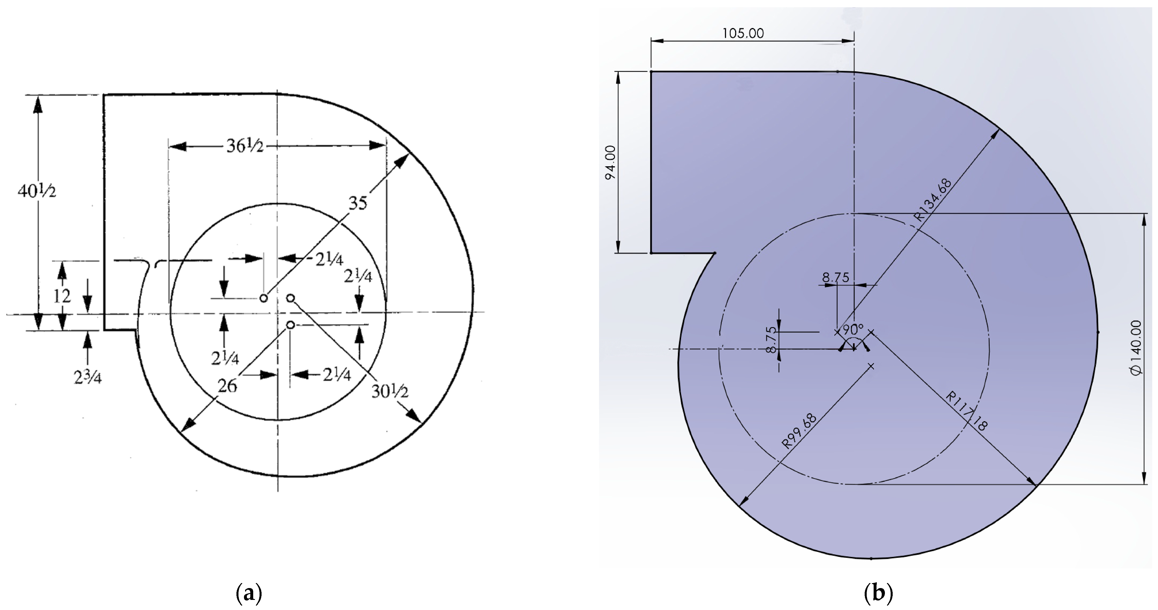
Virtual experiments require a 3D model of the test object, so the fan is modeled using the SolidWorks computer simulation software (version 2019; manufacturer: Dassault Systèmes SE; location: 3DS Paris Campus, 10 Rue Marcel Dassault, 78140 Vélizy-Villacoublay, France). The geometry consists of two parts: the fan impeller and the housing. The dimensions of the model are based on the dimensions of the Ziehl-Abegg product [22]. The centrifugal fan housing has an adjustable radius with dimensions given in Frank P. Bleier’s Fan Handbook [23,24]. There is a diagram in the manual that describes the relationship between the diameter of the impeller (d₁) and the quarter radii of the fan housing. The centers of curvature of the envelope helix are located more than 0.0625⋅${\mathrm{d}}_1$ from the origin of the coordinates. The radii of convexity of the quarters (moving away from the housing outlet) are 0.712⋅${\mathrm{d}}_1$, 0.837⋅${\mathrm{d}}_1$, and 0.962⋅${\mathrm{d}}_1$. The outer perimeter smoothly transitions. The height of the fan body is taken to be 86 mm, and the width of the outlet channel is 94 mm, paying attention to the dimensions of products common on the market (Figure 1). Figure 1 shows a comparison between a typical impeller body and the one used in this work. Frank P. Bleier’s Fan Handbook provides a schematic diagram describing the relationship between the impeller diameter and the quarter radii of the fan casing.

The impeller model consists of two lower and upper discs, with 33 blades arranged between them. In conformity with the genuine fan design, the overall impeller height measures 60 mm. During geometry optimization, angles ${\beta }_1$ and ${\beta }_2$ (which represent the vane’s leading and trailing angle, respectively) are considered parametric model elements that can be adjusted. The values for ${\mathrm{D}}_1$ and ${\mathrm{D}}_2$ are considered fixed at 116 mm and 140 mm, respectively. As these values remain constant, the model possesses an adequate number of parameters to effectively define the blade’s shape (Figure 2).

A model of an EC (electronically commuted) motor is built using the dimensions provided in the Ziehl-Abegg manufacturer’s catalog [22]. This model accurately simulates the working conditions of an actual impeller attached to an exterior rotor. A general model of the centrifugal fan used in the study is created by combining the individual modeled parts. The primary factors determining the shape of the air blade are the angles at which the blade starts (${\beta }_1$) and ends (${\beta }_2$). To ensure a consistent flow on the blade’s surface under specific working conditions, it is crucial to accurately select the values for these parameters. This study focuses on fans equipped with impellers that have forward-facing blades. This means that for angles ${\beta }_1$ and ${\beta }_2$, which represent the specific blade positions, a boundary condition is set, stating that angles must be less than 90°. To determine the optimal blade parameters, separate evaluations are conducted for the first and second design points. The values of the ${\beta }_1$ and ${\beta }_2$ parameters are adjusted in increments to identify the most favorable outcomes. Over a thousand impellers, each with unique geometry parameters, are tested during this study. The efficiencies of impellers are calculated at specific design points, and the impellers with the highest total efficiency are discovered.

The initial operating point reflects the peak power consumption as the fan operates at 1930 rpm with maximum air flow. This condition occurs because there is no static pressure resistance in the system. The fan that has the highest energy consumption is the one with blades facing forward. The most efficient fan at this operating point, where the blade angles range from 0° to 90°, is regarded as the most optimal. Calculating the velocity triangles at the front of the blade enables narrowing down of the parameter ${\beta }_1$ identification range. The assumption is made that the ideal angle of the leading edge of the blade is aligned with the direction of the flow velocity vector. Determining angle ${\beta }_2$ proves impossible due to the dependence of the outgoing flow vector on the blade’s rear angle. Consequently, it is only be feasible to calculate a portion of the flow component, leading to insignificant results. Additionally, to calculate the value of the trailing angle (${\beta }_2$), it is essential to assess the coefficients of flow losses, which can only be accurately determined through testing Cory [25].

Air is sucked out of the central zone and routed between the two blades. Centrifugal force then pushes air towards the outer zone of the centrifugal fan. From a single blade’s perspective, air flow reaches its geometric basis and flows through the blade channel. The assumption made in this work is that the flow field is tangential to a blade’s profile at the initial point.

The purpose is to define the blade equation in a Cartesian coordinate system for further optimization of the process [26,27,28]. A Cartesian coordinate system {x, y} is defined with the y-axis containing the initial geometry point of the blade (Figure 2b). The profile of the blade can be assumed as a smooth function ($x=F\left(y\right)$); the velocity field of the flow is tangential, i.e., physical effects such as boundary layer or flow separation are ignored. The acceleration of the flow along the blade’s side is the sum of the normal and tangential accelerations [26,27,28].

$$a_n={\omega }^2\cdot \rho \cdot (\cos \alpha ,\sin \alpha )=\frac{v^2}{\rho }\cdot (\cos \alpha ,\sin \alpha )$$

(1)

$$a_t=\epsilon \cdot \rho \cdot (\cos \alpha ,\sin \alpha )=\dot{v}\cdot (\cos \alpha ,\sin \alpha )$$

(2)

$$a=a_n+a_t$$

(3)

$$\ddot{x}=\dot{v}\sin \alpha +\frac{v^2}{\rho }\cdot \cos \alpha$$

(4)

where $v$ is the instantaneous velocity in a defined coordinate system, ρ is the radius of the curvature, ω is the angular velocity, and ε is the angular acceleration.

Derivatives of smooth function $x=F\left(y\right)$ have to be defined to express velocity and acceleration [26,27,28].

$$\dot{x}=\dot{F}(y)\dot{y}$$

(5)

$$\ddot{x}=\ddot{F}(y)\cdot y^2+F(y)\cdot \ddot{y}$$

(6)

where the first and second derivatives are velocity and acceleration, respectively [26,27,28].

$$v^2={\dot{x}}^2+{\dot{y}}^2=(1+F^2(y))\cdot {\dot{y}}^2$$

(7)

$$2\cdot v\cdot v^2=2\cdot \dot{F}(y)\cdot \ddot{F}(y)\cdot {\dot{y}}^3+2\cdot (1+\dot{F^2}(y))\cdot \dot{y}\cdot \ddot{y}$$

(8)

If $\tan \alpha =-F\left(y\right)$, then simple trigonometric expression of angle α is as follows [26,27,28]:

$$\frac{\mathit{tan}\alpha }{\sqrt{1+{\mathit{tan}}^2\alpha }}=\frac{\mathit{sin}\alpha }{\mathit{cos}\alpha }\cdot \frac{1}{\sqrt{\frac{{\mathit{cos}}^2\alpha +{\mathit{sin}}^2\alpha }{{\mathit{cos}}^2\alpha }}}=\frac{\mathit{sin}\alpha }{\mathit{cos}\alpha }\cdot \left|\mathit{cos}\alpha \right|=\mathit{sin}\alpha \cdot \frac{\left|\mathit{cos}\alpha \right|}{\mathit{cos}\alpha }=\mathit{sin}\alpha =\frac{-\dot{F}\left(y\right)}{\sqrt{1+{\dot{F}}^2\left(y\right)}}$$

(9)

$$\frac{1}{\sqrt{1+{\mathit{tan}}^2\alpha }}=\frac{1}{\sqrt{\frac{{\mathit{cos}}^2\alpha +{\mathit{sin}}^2\alpha }{{\mathit{cos}}^2\alpha }}}=\frac{1}{\sqrt{\frac{1}{{\mathit{cos}}^2\alpha }}}=\left|\mathit{cos}\alpha \right|=\mathit{cos}\alpha =\frac{1}{\sqrt{1+{\dot{F}}^2\left(y\right)}}$$

(10)

These definitions and the assumption that $\ddot{F}(y)>0$ allow Equation (4) to be rearranged as follows [26,27,28]:

$$\dot{F}(y)\cdot (1+\dot{F^2}(y))\cdot \ddot{y}+\dot{F^2}(y)\cdot \ddot{F}(y)\cdot \dot{y^2}=0$$

(11)

At the points where velocity is equal to zero or $\dot{F}(y)=0$, Equation (11) is satisfied; therefore, at the points where $\dot{F}(y)\ne 0$, the equation becomes the following [26,27,28]:

$$(1+\dot{F^2}(y))\cdot \ddot{y}+\dot{F}(y)\cdot \ddot{F}(y)\cdot \dot{y^2}=0$$

(12)

Equation (12) is a nonlinear differential equation and can be used in two cases. In the first case, if the blade profile is assigned by function $F\left(y\right)$, then using the last equation, i.e., the profile itself, the law of motion ($y=y\left(t\right)$) along the blade side can be calculated. The second case involves particular motion ($y\left(t\right)$) assignment; then, the equation allows for the calculation of the blade profile ($F\left(y\right)$) itself.

Optimization Problem Definition

A particular law of motion ($y=y\left(t\right)$) is required in the optimization process to achieve the best possible fan efficiency; therefore, boundary conditions $g$ and $h$ are essential and have to be defined. It follows that [26,27,28]

$$y=g\left(y\right)$$

(13)

and

$$\ddot{y}=\dot{g}\left(y\right)\cdot g\left(y\right)$$

(14)

It has to be noted that for geometrical assumptions, the boundary condition can be defined as $F\left(h\right)=0$, where $(0,h)$ are Cartesian coordinates of the initial point of the impeller blade. The derivative of the boundary condition $\dot{F}(y,h)=c_0$ comes from the physical assumption about the tangential flow at the initial point of the blade. The slope of the flow field at the impeller inlet is noted as $c_0$. These conditions allow for the formulation of the differential optimization problem as follows [26,27,28]:

$$\left\{\begin{array}{c}\dot{g}(y)\cdot g(y)\cdot (1+\dot{F^2}(y)+g^2(y)\cdot \dot{F}(y)\cdot \ddot{F}(y)=0)\\ F(h)=0\\ \dot{F}(y,h)=0\end{array}\right\}$$

(15)

The boundary conditions can be easily revised, considering that the blade has zero curvature, that is, $\ddot{F}(y)=0$ for every coordinate point. Then, according to Equation (15),

$$\dot{g}(y)\cdot g(y)\cdot (1+\dot{F^2}(y))=0$$

(16)

It is obvious that $\dot{g}(y)=0$ at every coordinate point, that is, $y(t)=At+B$ is equal to $\ddot{y}=0$. From the opposite point of view, if $y(t)$ is linear in time, then boundary condition $g(y)=0$ for every coordinate point, and the differential formulation becomes the following:

$$g^2(y)\cdot \dot{F}(y)\cdot \ddot{F}(y)=0$$

(17)

As a result, $\ddot{F}(y)=0$, and from Equation (5), it follows that $x(t)$ is linear as well. This drives optimization considering constant speed along the airflow direction.

Using the principle of superposition and fixing the blade, the flow at the leading edge of the blade (${\omega }_1$) can be described in terms of the centrifugal ($c_1$) and tangential ($u_1$) velocity vectors Darvish [28]. If the impeller under study has relatively similar operating conditions to the product discussed by the Ziehl-Abegg manufacturer [22], then the fan air flow rate ($v_p$) in this duct is determined by Equation (18), where the area of the intake duct ($A_p$) and the amount of air blown by the Ziehl-Abegg fan at the design point ($Q_p$) are expressed as follows:

$$v_{pi}=\frac{Q_{pi}}{A_p} \mathrm{or} v_{p1}=\frac{Q_{p1}}{A_p}=13.15 \mathrm{m}/\mathrm{s}$$

(18)

When applying the flow continuity expression, the relationship between the velocity (${\upsilon }_{pi}$) and the area ($A_p$) of the inlet channel and that between the centrifugal velocity ($c_i$) at the leading edge of the impeller and the area ($A_1$) on the perimeter of $D_1$ are expressed. The components of the flow velocity vectors at the leading edge of the blade are then found as follows:

$$\frac{A_1}{A_p}=\frac{{\upsilon }_{pi}}{c_i}$$

(19)

$$c_i=A_p·v_{pi}/A_1$$

(20)

When calculating the area of the channel at $D_1$, the part of the channel blocked by the blades is not considered, since the calculations are used only to reduce the range of the search field. Next, the component of the flow velocity vector in the tangential direction ($u_1$) with respect to $D_1$ is calculated as follows:

$$u_1=D_1·\omega /2$$

(21)

Knowing the values of both velocity vector components, the leading edge of the blade can be expressed by ${\beta }_1$ as follows:

$${\beta }_i={\mathrm{t}\mathrm{a}\mathrm{n}}^{-1}\frac{c_i}{u_i} \mathrm{or} {\beta }_1={\mathrm{t}\mathrm{a}\mathrm{n}}^{-1}\frac{c_1}{u_1}=29.3°$$

(22)

By conducting these calculations and making certain assumptions, the size of the search field for the initial simulations can be reduced. This is because there is no need to check the ${\beta }_1$ parameter throughout the entire section if the assumption regarding the blade and flow angle coincidence is confirmed. To discover the optimal impeller design, a parametric analysis is conducted, generating a diverse range of test fans. In this analysis, the parameter values are altered as per the table’s guidelines.

The purpose of this study is to verify whether the performance curves of fan impellers optimized at two specific operating points differ. Different operating modes lead to changes in geometry, which are reflected in the performance curves accordingly. Such changes are determined by the fact that when the operating mode changes, the airflow velocity vectors surrounding the blade are redistributed—in other words, the components of the velocity triangle and the angle changes at which the blade is oriented to the flow Singh and Nestmann [29]. To test this hypothesis, 2 design points (DPs) are set, namely (1) the working section of maximum load and maximum power consumption (1st DP) and (2) the working range of maximum full efficiency of the fan (2nd DP) (Figure 3).

The power consumption of the fan directly depends on the air flow, so the maximum power consumption is observed at the lowest system resistance. When the system pressure gain approaches 0, the fan operates in the zone of maximum resistance due to the maximum amount of air particles flowing over the surface of the blades Chunxi et al. [30]. This operating point (1st DP) is chosen for the first optimization step.

The most efficient operating point of a fan can be described in terms of static or dynamic efficiency. According to the typical characteristic curves of the test object, the static efficiency curve approaches 0 when the fan works in the maximum power zone. In the theoretical case, when the fan is operating in this mode, there is no static system resistance, so it is not appropriate to use static efficiency at this particular point. Meanwhile, the dynamic efficiency at this point is not be equal to 0, since the generated flow has its own energy. Therefore, dynamic efficiency is used as the main efficiency criterion in further research. For the second optimization, the maximum efficiency point (2nd DP) is selected.

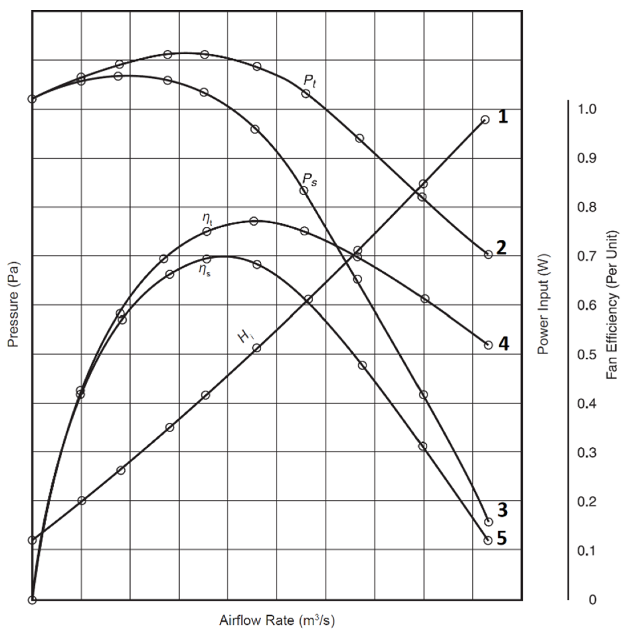
The impeller diameter selected in this article is based on the most common fans. One manufacturer of widely used fans is Ziehl-Abegg. The Ziehl-Abegg fan with an impeller diameter of 140 mm from the manufacturer’s freely accessible electronic catalog is chosen for this study Ziehl-Abegg SE [22]. A third point is selected from the graph. This point describes the operating point at which the maximum amount of air flow is blown, as there is no increase in system static resistance (Figure 4). As shown in the standard curves above, a fan operating at this point will consume the maximum amount of power (compared to the constant speed graph), so it is assumed that the impeller will rotate at 1930 rpm in the virtual tests.

Considering Figure 3 and Figure 4, the operating modes are evaluated for each design point (DP) separately so that the DP reflects/shows the operation of the fan for different fan conditions. Based on this, it is observed that it is inappropriate to calculate the efficiency for all DPs in general, considering all these design points.

The 3D model of the fan is created using SolidWorks software (version is provided in Section 2). The Flow Simulation extension of this software is used to perform flow simulations, so the virtual geometry is created according to the dimensions of the real product and in accordance with the geometric coefficients specified in Frank P. Bleier’s Fan Handbook [23,24]. In this model, the geometry parameters for the leading and trailing angles of the blades (${\beta }_1$, ${\beta }_2$) are entered, which will be changed during the parametric simulations.

The optimization of the geometry of the impeller is performed by changing the parameters of the leading and trailing angles of the blade (${\beta }_1$, ${\beta }_2$). Optimal geometry parameter values are searched for at two design points by changing the boundary conditions of the model. At the end of this stage, two different centrifugal fan impellers are obtained, the geometry parameters of which are selected according to the optimal values of the parametric simulation for each operating mode. The efficiency characteristics and performance curves of both obtained impellers are identified in the following phase. Graphs describing the operating ranges of the fan at 1500, 2000, and 2500 rpm are presented, since these rev limits are the actual operating zones. Conclusions about the impact of the design point choice on the fan’s operating modes are drawn by comparing these graphs.

The algorithm is selected based on the standard. ANSI/AMCA standard 210-16 [31] provides equations for calculating fan efficiency. Based on this standard, the calculation is carried out in the appropriate order, and the efficiency and properties are calculated. Efficiency is also viewed as an estimate of the existing geometry. For each fan, 2 efficiencies can be calculated, namely full and static efficiencies. The difference is that either absolute or static air pressure is measured and substituted into the same equation as follows:

$$\eta =\frac{QP{K}_P}{H_i}$$

(23)

where $\eta$ is fan efficiency, $Q$ is the airflow rate (m³/s), $P$ is flow pressure (Pa), $K_P$ is the compression ratio, and $H_i$ is the current power used by the fan motor (W).

Several simplifications and assumptions can be made with respect to Equation (23). First, the compressibility factor can be removed because it is used at high Mach speeds, and in the simulations, the air flow is assumed to be incompressible. Second, the electric motor that is used to spin the fan is not pulled into the simulation, so the power consumption is assumed to be equal to the aerodynamic drag power. Under these assumptions, the standardized equation can be rewritten as an efficiency equation suitable for use in this study as follows:

$$\eta =\frac{QP}{P_{req}}$$

(24)

where $\eta$ is fan efficiency, $Q$ is the airflow rate (m³/s), $P$ is flow pressure (Pa), and $P_{req}$ is the power needed to overcome air resistance (W).

The objective of the optimization performed in this paper is to maximize efficiency (Equation (24)) at various design points. The search procedure identifies the optimal value of the objective function throughout the search space, i.e., the maximum value. The search procedure utilized in this work is a linear search. This sequential algorithm goes through all elements in the list. The algorithm considers every element as a potential maximum of the objective function, but since actual value is unknown in advance, the entire search space is searched. At the end, the maximum value is sorted out.

Some additional materials can also be assessed for future research. These articles encompass various aspects of engineering research, including fan blade optimization, comparison of numerical models for fluid-viscous dampers, and the application of deep learning in structural health monitoring.

The impeller design of a centrifugal fan with blade optimization was investigated by Lee et al. [32]. They mentioned that the width of the impeller is almost linearly related to the impeller’s total generated head. Aerodynamic and aeroacoustic optimizations for the design of a centrifugal fan with forward-curved blades were presented by Heo et al. [33]. Their flow analysis of a centrifugal fan with forward-curved blades was conducted by solving three-dimensional steady and unsteady Reynolds-averaged Navier–Stokes equations using the shear-stress transport turbulence model.

Lee et al. [32] and Heo et al. [33] investigated the optimization of centrifugal fan blades to enhance aerodynamic and aeroacoustic performance. Lee et al. [32] demonstrated that optimizing blade geometry can significantly improve fan efficiency, while Heo et al. [33] achieved a reduction in noise levels through aeroacoustic optimization. Both studies highlight the importance of considering various design parameters and employing computational fluid dynamics simulations for the development of efficient and low-noise fans.

Cucuzza et al. [34] compared numerical models for fluid-viscous dampers and used genetic algorithms to evaluate damper performance. Their results indicate that the proposed nonlinear Bingham model outperforms traditional linear and nonlinear models in terms of prediction accuracy. This study emphasizes the significance of assessing different numerical models and implementing advanced optimization techniques for effective damper design and analysis.

Rosso et al. [35] conducted a review of deep learning applications in structural health monitoring, illustrating the potential of data-driven approaches for the monitoring and maintenance of structural integrity. They presented several case studies demonstrating the successful implementation of deep learning techniques, such as convolutional neural networks and recurrent neural networks, in detecting and classifying structural damage. This research underscores the importance of leveraging interdisciplinary methodologies and emerging technologies to address engineering challenges.

Aerodynamic optimization of a multi-blade centrifugal fan based on an extreme learning machine surrogate model and a particle swarm optimization algorithm was presented by Meng et al. [36]. In this study, the authors employed an Extreme Learning Machine (ELM) surrogate model and a Particle Swarm Optimization (PSO) algorithm to explore various blade designs and identify optimal configurations. The ELM surrogate model was used to approximate the objective functions, while the PSO algorithm facilitated the optimization process. This research contributes to the growing body of work on advanced computational techniques for optimizing the aerodynamic performance of centrifugal fans. By showcasing the potential of combining surrogate modeling and optimization algorithms, the authors demonstrated a promising approach for improving fan efficiency and performance.

3. Results

If the tested impeller has relatively similar operating conditions to those of the Ziehl-Abegg product [22], it is assumed that the area of the fan air inlet is $A$ = 0.01056 m² and, according to Equation (18), the flow velocity is ${\upsilon }_p$ = 13.15 m/s (at the first design point, the airflow rate blown by the Ziehl-Abegg fan is $Q$ = 500 m³/h).

The aim of the impeller geometry optimization is to maximize full efficiency by changing the values of the leading and trailing angles of the blade. To calculate the efficiency, additional parameters are put into the calculation domain. The average total air pressure and the airflow rate are measured in the outlet channel, and the torque criterion is required. The product of the torque about the Y axis and the angular velocity allows for estimation of the power requirement for the rotation of the impeller, showing that the power requirement is equal to the aerodynamic resistance Lasauskas [37]. These additional objectives provide all the variables needed for the fan efficiency calculations according to Equation (19).

Calculations are performed in two steps. First, the optimal geometry of impeller blade is determined; then, numerical experiments are performed to determine the efficiency of the fan at various DPs by simulating real working conditions. Geometry optimization results are presented in Section 3.1, and calculation results and analysis of the optimized fan are provided in Section 3.2. The results are provided in two sections for geometry optimization and performance analysis.

3.1. Fan Blade Leading- and Trailing-Angle Optimization

The main parameters of the geometry of the impeller are the leading and trailing angles (${\beta }_1$, ${\beta }_2$) of the blade. Optimal values of these parameters ensure uniform air flow on the surface of the blade under specific working conditions. In this study, the focus is put on impellers with forward-facing blades; therefore, a boundary condition is introduced for the angles (${\beta }_1$, ${\beta }_2<90°$). The optimal blade parameters are calculated separately for the first and second design points (DPs), changing the values of the ${\beta }_1$ and ${\beta }_2$. This phase of the efficiency study includes more than 1000 iterations of different geometry parameters.

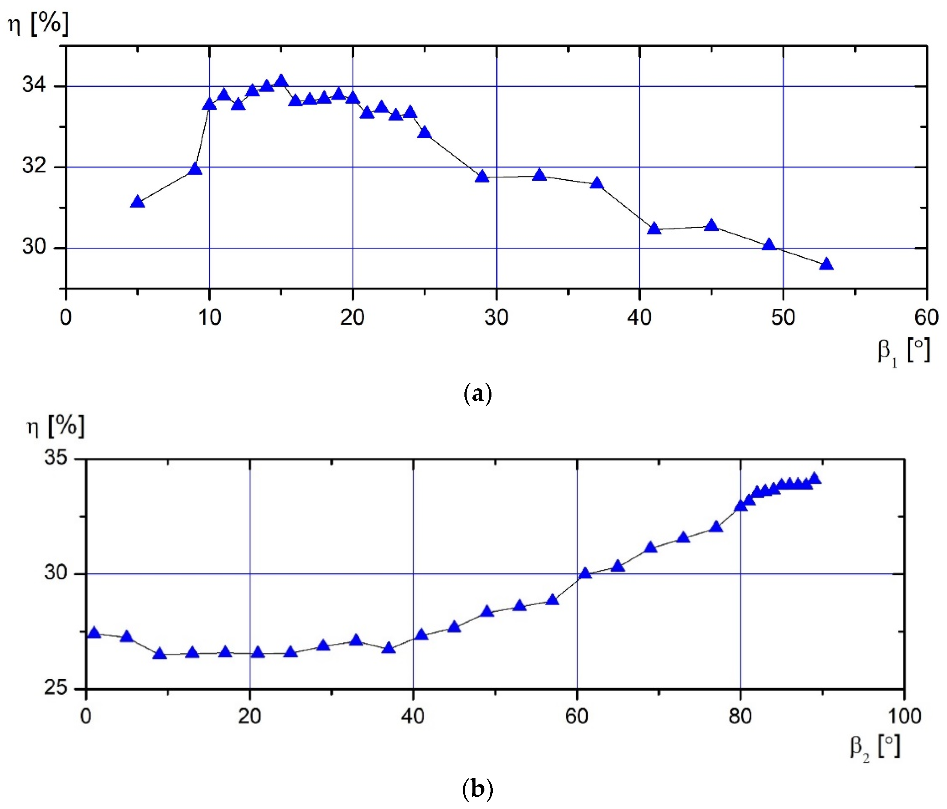
The graphs presented in Figure 5 show the efficiency values at specific values of the geometry parameters; maximum efficiency is achieved at ${\beta }_1=15°$ and ${\beta }_2=89°$. It is observed that the value of ${\beta }_1$ calculated by making preliminary assumptions differs from the optimal value obtained during virtual tests. This can be explained by the fact that the generated fan flow determined in the performance curve differs by almost 2 times from the real manufacturer’s device. It can be seen from the efficiency dependence on ${\beta }_2$ shown in the data graph (Figure 5b) that the highest values are reached at the edge of the test interval. Such results are expected, since fans with forward-facing blades are less efficient than those with backward-facing blades (their ${\beta }_2>90°$) Montazerin et al. [38].

The second design point (DP) corresponds to the most efficient point of the operating mode, when the fan operates at an angular speed of 1930 rpm. At this point, the fan reaches the peak of its efficiency; therefore, there the most optimal air flow into the system appears with a certain pressure increase. Pressure gain is determined from the results of the first optimization. The peak efficiency of the first fan is found to occur at a flow rate of 190 m³/h and a resistance of 75 Pa, with the fan operating at an angular speed of 2000 rpm. To maintain the integrity of the work, it is assumed that the device will have to overcome a system pressure increase of 70 Pa at the second design point. It is assumed that the fan will create an air flow rate of 180 m³/h when operating at a speed of 1930 rpm.

After performing the calculations, the components of the airflow velocity vector at the impeller blade with the initial diameter are found. According these results, the optimal value of β₁ at the second design point is calculated as 11.48°. These calculations are also performed under the assumption that the front part of the blade is oriented towards the incoming air flow.

The graphs presented in Figure 6 show all the impellers with different geometries tested during the virtual test. The data are grouped according to the studied parameters (${\beta }_1$ and ${\beta }_2$) to determine the distribution of the full efficiency of the studied cases at specific values of the parameters. The geometry parameter (${\beta }_1$) of the most efficient impeller reaches 14°, and ${\beta }_2$ does not stop growing in the entire studied interval. This value of the rear blade angle is also discussed with respect to the results obtained during the optimization at the first design point. Observing the data that represent the highest full efficiency at specific values of ${\beta }_1$ and ${\beta }_2$, it can be observed that the impeller with the geometry parameters of ${\beta }_1=12°$ and ${\beta }_2=88°$ achieves the highest efficiency.

3.2. Study of Fan Operating Curves

The purpose of this study is to determine the influence of the design points for optimization on the operating curves of the fan; therefore, virtual tests with optimized impellers are performed in this section. Curves of the dependence of performance and efficiency on the flow rate are determined for both optimized fans. Parameters are calculated at the angular speeds of 1500, 2000, and 2500 rpm, as these are typical operating modes for fans with 140 mm diameter impellers. The curves are determined at an ambient air temperature of 20.05 °C and a pressure of 101,325 Pa on the air-intake side of the fan.

The methodology discussed in the ANSI/AMCA 210-16 fan aerodynamic test specifications is used to determine the performance curves. Virtual tests are performed by increasing the system resistance (static pressure) and recording the operating parameters of the fan at the selected angular speed. At each point of the operating curve, the fan’s efficiency parameters are calculated, according to which the influence of geometry parameters is monitored.

3.2.1. Operating Curves at First Design Point

After the optimization of the geometry of the first design point (DP), it is determined that the impeller with geometry parameters of β₁ = 15° and β₂ = 89° works most efficiently in this mode. Performance and efficiency curves are determined for a fan with these geometry parameters.

The performance curve indicates the working range of the fan, in addition to indicating the amount of air flow at a specific pressure gain (resistance) of the system. In the presented graphs, the horizontal X axis shows the airflow rate (m³/h) created by the fan, and the vertical Y axis shows the static pressure increase of the system (Pa). These characteristic curves are determined at different angular speeds, namely 1500, 2000, and 2500 rpm. These speeds are chosen based on the operating speeds of real fans with 140 mm diameter impellers.

As the angular velocity increases, the flow rate and maximum static pressure created by the fan increase as well. According to fan laws, the flow is directly proportional to the change in angular velocity. A quadratic dependence is also observed between static pressure and angular velocity at different operating points Brown [39]. The following dependencies can be observed in the graph obtained during the virtual tests, which lead to the assessment that the flow simulations were performed correctly and reflect the dependencies of physical tests.

From the obtained results, it can be observed that the fan at the first DP can create airflow rates of 205, 273, and 345 m³/h when operating at angular speeds of 1500, 2000, and 2500 rpm, respectively. These points describe the extreme operating modes, since the device works only in the absence of system resistance. The maximum pressures generated by the fan reach 51.5, 99, and 145.5 Pa, respectively.

In all the performance curves (Figure 7), the unstable zone of the operating mode can be observed. In this zone, the fan curve becomes flat; therefore, the minimal change in system pressure has a significant effect on the flow rate. When working in this mode, the number of vibrations increases, and the efficiency of the device decreases Gustafson [40].

The fan’s efficiency curve defines how the fan can generate the airflow rate at a specific system resistance. In the presented graphs, the horizontal X axis shows the airflow rate (m³/h), and the vertical Y axis shows the static efficiency (%), which is calculated according to the equations discussed previously. The obtained data show that the maximum efficiencies of the fan optimized at the first DP reach 43.2, 45.6, and 46.2% when the device works at angular speeds of 1500, 2000, and 2500 rpm, respectively. It can also be observed that as the angular speed of the fan increases, the maximum static efficiency increases as well.

Performance and efficiency curves should be analyzed together, since their points can be described according to the three coordinates of airflow rate, pressure, and efficiency. It can be seen that the static efficiency of the fan is equal to 0% when the maximum airflow rate is generated at a system resistance of 0 Pa. As the system pressure increases, the efficiency increases until it reaches its maximum value. As the resistance continues to rise, the fan enters an unstable operating zone, where the static efficiency begins to drop until it reaches 0%. At this extreme point, the fan no longer creates air flow but only maintains the pressure increase in the system.

By combining the performance and efficiency graphs, the exact operating mode of the most efficient fan can be determined. The fan at the first DP with an angular speed of 1500 rpm is most efficient when it produces a flow rate of 125 m³/h at a system resistance of 50.25 Pa. Operating at 2000 rpm, the maximum theoretical efficiency of the fan is achieved at a pressure of 96.5 Pa, with an air flow of 155 m³/h. Operating at the highest tested angular speed (2500 rpm), the fan achieves maximum efficiency at a system resistance of 143.15 Pa, creating a flow rate of 198 m³/h.

3.2.2. Operating Curves at Second Design Point

After selecting the optimal geometry parameters at the second design point (DP), it is determined that the impeller with geometry parameters of β₁ = 12° and β₂ = 88° works most efficiently. Performance and efficiency curves are determined for a fan with these blade geometry parameters.

The characteristics of the fan of the second DP are determined analogously to the curves of the fan at the first DP using SolidWorks software (version is provided in the Section 2) extension “Flow Simulation”. In the virtual computational domain, the pressure increment of the system is varied, recording the flow dependence at each point.

The determined performance curves (Figure 8) show the flow rate (m³/h) produced by the fan on the horizontal X axis and the static resistance (Pa) of the system on the vertical Y axis. From the obtained operating curves, it can be seen that the maximum flows generated by the fan at the second DP reach 200, 271, and 343 m³/h when the device operates at 1500, 2000, and 2500 rpm, respectively. The maximum static pressure developed by this fan is 50 Pa at an angular speed of 1500 min⁻¹ and 94.5 and 143.5 Pa at angular speeds of 2000 and 2500 min⁻¹, respectively.

During the virtual tests, the power consumption of the fan is recorded, and the static efficiency is calculated at each point. The graph presented in Figure 8a shows the dependence of static efficiency of the airflow rate. The horizontal X axis shows the amount of air flow (m³/h) blown by the fan, and the vertical Y axis shows the static efficiency (%). It can be seen that at an angular speed of 1500 rpm, the maximum static efficiencies of the fan reach 41.3% and 44.1 and 44.5% at angular speeds of 2000 and 2500 rpm, respectively.

It should be noted that as the angular speed increases, the value of the maximum efficiency increases as well. Peak static efficiency increases by 2.8% from 41.3 to 44.1% as the speed changes from 1500 to 2000 rpm. As the angular velocity changes from 2000 to 2500 rpm, the efficiency gain drops to 0.4%. Thus, it cannot be stated that the increase in values of angular velocity and static efficiency has a direct relationship.

By combining the graphs of the performance and efficiency of the fan at the second DP (Figure 8), it is possible to determine the theoretically most efficient operating modes at the studied angular velocities. Operating at an angular speed of 1500 rpm, the fan achieves maximum efficiency at a system static pressure resistance of 47.5 Pa, producing a flow rate of 123 m³/h. At an angular speed of 2000 rpm, the fan optimized at the second DP is most efficient when blowing 156.5 m³/h at 90 Pa static resistance. Operating at the highest tested angular velocity, the fan reaches its theoretical efficiency peak at a pressure of 139 Pa, when it produces an airflow rate of 208 m³/h.

Considering the results, known literature can be also mentioned. A study published by Chinese researchers in the International Journal of Mechanical Sciences describes the influence of eccentricity on the performance characteristics of a centrifugal fan’s leading edge Wang et al. [3]. The results of the experiments led to the conclusion that the data obtained during numerical simulations correlated with the results obtained during real experiments. There was a noticeable difference of 3.05% in the data results when evaluating the increase in static pressure, namely 348.08 Pa from simulations and 337.78 Pa from the experiment. The authors noted that the optimization criteria were appropriate, as the optimized wing’s performance characteristics significantly outperformed those of the initial wing. These results were achieved without increasing the level of noise emitted by the device.

Researchers from Sherbrooke University in Canada Lehocine et al. [5] utilized a fully automated cyclic process for the design of an eccentric centrifugal fan blade. The researchers noted that as restrictions and requirements for air quality and ventilation systems increase, it becomes challenging to find space for device improvements. Their geometry design process, using meta-modeling, allows for the optimization of up to seven different geometry parameters [36]. The optimization meta-model algorithm developed by the researchers improved blade efficiency from 2.35% to 5.71%. Optimization using “OpenFOAM” software (version is provided in Section 2) enhanced efficiency from 3.27% to 4.22%. The authors pointed out that the inclusion of a second group of parameters in the calculation algorithm led to a 4.1% improvement in efficiency compared to the introduction of the additional group with optimal geometry parameters.

Work conducted by researchers from China introduced the process of optimizing fan blades by selecting an optimized blade profile (Zhou et al. [6]). The authors noted that in all fan optimization studies, there is a plethora of geometry parameter evaluations conducted, making the analysis resource-intensive due to the vast number of possibilities. For this reason, their study specifically focused on the blade geometry to optimize the arc-shaped profile. It was observed that the overall efficiency increased by 3.1%, and the airflow rate increased by 1.4 m³/min when comparing the optimized profile blade with the initial profile. The improvement in criteria was achieved by changing the angles of the starts and ends of the profile strings, with the greatest differences observed at the trailing edge of the profile, which was highly curved.

From this review of scientific literature, it can be seen that the results of the experiments described in the article correlate with global practice, i.e., comparing the performance curves of the fans resulted in a 0.56–2.45% higher airflow rate for the fan optimized at the first DP compared to the maximum flow rate of the fan at the second DP in the absence of system static resistance. Reviewing the established operating characteristics at the same fan speeds, it was observed that the fan optimized at the first DP supported 1.4–4.5% higher static system pressure increases than the test object designed at the second DP.

4. Summary and Discussion

As it mentioned before, the aim of impeller geometry optimization is to maximize full efficiency by changing the values of the leading and trailing angles of the blade. Considering the results and to represent a summary of research, the following key findings are presented:

• It is determined that at the point of maximum power (1st DP), the highest achievable value of the static efficiency of the optimized fan, which is in the medium flow-rate zone (56.7–61.4% of the maximum amount of blown air at the tested speeds), is 3.2–4.4% higher compared to the fan at the second DP when the test objects run at the same speed.
• The results collected during the virtual tests show that the test object, the geometry parameters of which are selected for the second DP, exhibits up to 12.5% higher static efficiency than the fan at the first DP operating with a low amount of blown air (11.1–35% of the maximum flow) and in the zone of high static system pressure gain (95.2–99.4% of the maximum sustained system resistance gain).
• Comparing the performance curves of the fans results in a 0.56–2.45% higher airflow rate for the fan optimized at the first DP compared to the maximum flow rate of the fan at the second DP in the absence of system static resistance.
• Reviewing the established operating characteristics at the same fan speeds, it is observed that the fan optimized at the first DP supports 1.4–4.5% higher static system pressure increases than the test object designed at the second DP.
• Based on the results of this research, we recommend selecting the operating modes of the fan in the stable zone.

To represent future work, a brief discussion can be additionally provided. Although the optimization of the geometry of a centrifugal fan at different design points is reported in this work, there still exist unsolved problems. One problem is the improvement of numerical investigation; the possible use of the Navier–Stokes equation can be considered to solve this problem [8,9,10]. Another problem is fan research from the physical implementation perspective. In the Introduction, many problems were mentioned. Considering physical implementation, as well as the problems related to fan reliability, wear and failure research, stability and control, and vibration, could be the next research step in this field.

5. Conclusions

We note that in studies with the aim of improving the efficiency of fans, the most often selected parameters for optimization are the trailing and leading angles of the blades. Optimization of these geometry parameters of a centrifugal fan with forward-facing blades is also carried out in this study. The study is performed at two design points (DPs), which reflect maximum-power (1st DP) and high-efficiency (2nd DP) operating modes. Using the “Flow Simulation” extension of computer modeling program “SolidWorks” for flow simulations, two different research objects are obtained. It is found that at the first optimization point, when the test object operates at a speed of 1930 rpm and the system pressure is constant, the fan with a leading angle of the blade equal to 15° and a trailing angle of 89° works most efficiently. At the second DP, when the fan rotates at a speed of 1930 rpm and the static pressure increase of the system reaches 70 Pa, the impeller with ${\beta }_1=12°$ and ${\beta }_2=88°$ develops the highest efficiency.

The performance and efficiency curves at speeds of 1500, 2000, and 2500 rpm are determined for both tested impellers. These speeds are chosen for the analysis by evaluating the operating modes of real 140 mm diameter centrifugal fans. By comparing the data obtained during the virtual flow simulations, the differences in the performance characteristics of the fans, which appear due to the influence of the selected design point, are determined.

References

- Noack, R.; Hassan, J. Europe never understood America’s love of air conditioning-until now. The Washington Post. 25 July 2019. Available online: https://www.washingtonpost.com/world/2019/06/28/europes-record-heatwave-is-changing-stubborn-minds-about-value-air-conditioning (accessed on 26 December 2023).
- Zhang, R.; Wang, K.; Li, Y.; Li, J. Aerodynamic optimization of squirrel-cage fan with dual inlet. Int. J. Fluid Mach. Syst. 2018, 11, 234–243. [Google Scholar] [CrossRef]
- Wang, K.; Ju, Y.; Zhang, C. Experimental and numerical investigations on effect of blade trimming on aerodynamic performance of squirrel cage fan. Int. J. Mech. Sci. 2020, 177, 105579. [Google Scholar] [CrossRef]
- ISO 5801; Fans Performance Testing Using Standardized Airways. ISO: Geneva, Switzerland, 2017.
- Lehocine, A.E.; Poncet, S.; Fellouah, H. Optimization of a squirrel cage fan. Prog. Can. Mech. Eng. 2021, 4, 1–6. [Google Scholar] [CrossRef]
- Zhou, S.; Yang, K.; Zhang, W.; Zhang, K.; Wang, C.; Jins, W. Optimization of multi-blade centrifugal fan blade design for ventilation and air-conditioning system based on disturbance CST function. Appl. Sci. 2021, 11, 7784. [Google Scholar] [CrossRef]
- Ding, H.; Chang, T.; Lin, F. The influence of the blade outlet angle on the flow field and pressure pulsation in a centrifugal fan. Processes 2020, 8, 1422. [Google Scholar] [CrossRef]
- Kim, K.Y.; Seo, S.J. Shape optimization of forward-curved-blade centrifugal fan with Navier-Stokes analysis. J. Fluids Eng. Trans. ASME 2004, 126, 735–742. [Google Scholar] [CrossRef]
- Kim, K.-Y.; Seo, S.-J. Application of Numerical Optimization Technique to Design of Forward-Curved Blades Centrifugal Fan. JSME Int. J. Ser. B 2006, 49, 152–158. [Google Scholar] [CrossRef]
- Heo, M.-W.; Kim, J.-H.; Kim, K.-Y. Design Optimization of a Centrifugal Fan with Splitter Blades. Int. J. Turbo Jet Engines 2015, 32, 143–154. [Google Scholar] [CrossRef]
- Zhang, L.; Wang, S.L.; Hu, C.X.; Zhang, Q. Multi-objective optimization design and experimental investigation of centrifugal fan performance. Chin. J. Mech. Eng. 2013, 26, 1267–1276. [Google Scholar] [CrossRef]
- Huang, C.H.; Hung, M.H. An optimal design algorithm for centrifugal fans. Theoretical and experimental studies. J. Mech. Sci. Technol. 2013, 27, 761–773. [Google Scholar] [CrossRef]
- Yu, S.C.M.; Chua, L.P.; Leo, H.L. The angle-resolved velocity measurements in the impeller passages of a model bio-centrifugal pump. Proc. Inst. Mech. Eng. Part C J. Mech. Eng. Sci. 2001, 215, 547–568. [Google Scholar] [CrossRef]
- Habashneh, M.; Cucuzza, R.; Domaneschi, M.; Movahedi Rad, M. Advanced elasto-plastic topology optimization of steel beams under elevated temperatures. Adv. Eng. Softw. 2024, 190, 1–14. [Google Scholar] [CrossRef]
- Cucuzza, R.; Domaneschi, M.; Rosso, M.M.; Martinelli, L.; Marano, G.C. Structural Optimization through Cutting Stock Problem. In Shell and Spatial Structures; Lecture Notes in Civil Engineering; Springer: Cham, Switzerland, 2023; pp. 210–220. [Google Scholar]
- Cucuzza, R.; Rosso, M.M.; Aloisio, A.; Melchiorre, J.; Giudice, M.L.; Marano, G.C. Size and shape optimization of a guyed mast structure under wind, ice and seismic loading. Appl. Sci. 2022, 12, 4875. [Google Scholar] [CrossRef]
- Rosso, M.M.; Cucuzza, R.; Aloisio, A.; Marano, G.C. Enhanced Multi-Strategy Particle Swarm Optimization for Constrained Problems with an Evolutionary-Strategies-Based Unfeasible Local Search Operator. Appl. Sci. 2022, 12, 2285. [Google Scholar] [CrossRef]
- Cucuzza, R.; Rosso, M.M.; Marano, G.C. Optimal preliminary design of variable section beams criterion. SN Appl. Sci. 2021, 3, 745. [Google Scholar] [CrossRef]
- Rad, M.M.; Habashneh, M.; Lógó, J. Reliability based bi-directional evolutionary topology optimization of geometric and material nonlinear analysis with imperfections. Comput. Struct. 2023, 287, 107120. [Google Scholar] [CrossRef]
- Habashneh, M.; Movahedi Rad, M. Optimizing structural topology design through consideration of fatigue crack propagation. Comput. Methods Appl. Mech. Eng. 2024, 419, 116629. [Google Scholar] [CrossRef]
- Rosso, M.M.; Cucuzza, R.; Di Trapani, F.; Marano, G.C. Nonpenalty Machine Learning Constraint Handling Using PSO-SVM for Structural Optimization. Adv. Civ. Eng. 2021, 2021, 6617750. [Google Scholar] [CrossRef]
- Ziehl-Abegg, S.E. Centrifugal Fans. Main Catalogue 2019. Künzelsau, Germany. Available online: https://www.ziehl-abegg.com/en/service/downloads (accessed on 26 December 2023).
- Bleier, F.P. Fan Handbook: Slection, Application and Design, 1st ed.; McGraw-Hill: New York, NY, USA, 1997; p. 640. [Google Scholar]
- Bleier, F.P. Fan Handbook: Selection, Application, and Design; McGraw-Hill: New York, NY, USA, 2018. [Google Scholar]
- Cory, W.T.W. 3—Air and gas flow. In Fans and Ventilation. A Practical Guide, 1st ed.; Elsevier Science: Amsterdam, The Netherlands, 2005; pp. 43–75. [Google Scholar] [CrossRef]
- Rouse, H. Fluid Mechanics for Hydraulic Engineers; Dover: New York, NY, USA, 1961. [Google Scholar]
- Courant, R. Differential and Integral Calculus. In First Published in Germany in 1930 as Vorlesungen über Differential-und Integralrechnung; Ishi Press: New York, NY, USA, 2011; Volume 1. [Google Scholar]
- Darvish, M. Numerical and Experimental Investigation of the Noise and Performance Characteristics of a Radial Fan with Forward-Curved Blades. Ph.D. Thesis, Technical University of Berlin, Berlin, Germany, 23 April 2015. Available online: https://depositonce.tu-berlin.de/items/54e100a4-72f6-4849-a9b8-c4e63e7d8616 (accessed on 26 December 2023).
- Singh, P.; Nestmann, F. Experimental investigation of the influence of blade height and blade number on the performance of low head axial flow turbines. Renew. Energy 2011, 36, 272–281. [Google Scholar] [CrossRef]
- Chunxi, L.; Ling, W.S.; Yakui, J. The performance of centrifugal fan with enlarged impeller. Energy Convers. Manag. 2011, 52, 2902–2910. [Google Scholar] [CrossRef]
- ANSI/AMCA standard 210-16; Laboratory Methods of Testing Fans for Certified Aerodynamic Performance Rating. ANSI: Washington, DC, USA, 2016.
- Lee, Y.T.; Ahuja, V.; Hosangadi, A.; Slipper, M.E.; Mulvihill, L.P.; Birkbeck, R.; Coleman, R.M. Impeller design of a centrifugal fan with blade optimization. Int. J. Rotating Mach. 2011, 2011, 537824. [Google Scholar] [CrossRef]
- Heo, M.-W.; Kim, J.-H.; Seo, T.-W.; Kim, K.-Y. Aerodynamic and aeroacoustic optimization for design of a forward-curved blades centrifugal fan. Proc. Inst. Mech. Eng. Part A J. Power Energy 2015, 230, 154–174. [Google Scholar] [CrossRef]
- Cucuzza, R.; Domaneschi, M.; Greco, R.; Marano, G.C. Numerical models comparison for fluid-viscous dampers: Performance investigations through Genetic Algorithm. Comput. Struct. 2023, 288, 107122. [Google Scholar] [CrossRef]
- Rosso, M.M.; Cucuzza, R.; Marano, G.C.; Aloisio, A.; Cirrincione, G. Review on Deep Learning. In Structural Health Monitoring, Bridge Safety, Maintenance, Management, Life-Cycle, Resilience and Sustainability—Casas; Casas, J.R., Frangopol, D.M., Turmo, J., Eds.; CRC Press: Boca Raton, FL, USA, 2022; pp. 309–315. [Google Scholar]
- Meng, F.; Wang, L.; Ming, W.; Zhang, H. Aerodynamics Optimization of Multi-Blade Centrifugal Fan Based on Extreme Learning Machine Surrogate Model and Particle Swarm Optimization Algorithm. Metals 2023, 13, 1222. [Google Scholar] [CrossRef]
- Lasauskas, E. Flight Principles: An Educational Book; Technika: Vilnius, Lithuania, 2008; p. 182. (In Lithuanian) [Google Scholar]
- Montazerin, N.; Akbari, G.; Mahmoodi, M. Developments in Turbomachinery Flow; Woodhead Publishing: Cambridge, UK, 2015; pp. 1–23. [Google Scholar] [CrossRef]
- Brown, R.N. Fan Laws, The User and Limits in Predicting Centrifugal Compressor Off Design Performance. In Proceedings of the 20th Turbomachinery Symposium; Turbomachinery Laboratories, Texas A&M University: College Station, TX, USA, 1991; pp. 91–100. Available online: http://oaktrust.library.tamu.edu/handle/1969.1/163545?show=full (accessed on 19 April 2024). [CrossRef]
- Gustafson, T. Understanding Centrifugal Fans. Plant Engineering HVAC 1995, File 2520, pp. 50–52. Available online: https://wesellfans.com/wp-content/uploads/2020/09/understanding-centrifugal-fans.pdf (accessed on 26 December 2023).
Figure 1.
The geometry of (a) is a typical example, and (b) represents the fan used in this work. (a) Typical 36.5-inch impeller body (Bleier [23,24]) (measurements presented in inches); (b) perimeter of the case model developed for the 140 mm impeller (measurements presented in mm).
Figure 2.
Fan blade geometry: (a) 3D model; (b) blade geometry design variables.
Figure 3.
Typical performance curves given in the ANSI/AMCA 210-16 standard: I—dependence of power consumption on flow rate; II—dependence of total pressure on flow rate; III—static pressure change from discharge; IV—dependence of full efficiency on debit; V—dependence of static efficiency on debit. Here reference points are numbered from 1 to 15.
Figure 4.
“RG14R-4IO.Z8.4R” performance curves of a centrifugal fan (Ziehl-Abegg SE [22]). Here reference curves are numbered from 1 to 5.
Figure 5.
Leading- and trailing-angle influence on full efficiency at 1st design point (DP): (a) influence of angle ; (b) influence of angle .
Figure 6.
Leading- and trailing-angle influence on full efficiency at 2nd design point (DP): (a) influence of angle ; (b) influence of angle .
Figure 7.
Operating parameters of optimized impeller at 1st design point (DP:) (a) performance; (b) static efficiency.
Figure 8.
Operating parameters of optimized impeller at 2nd design point (DP): (a) performance; (b) static efficiency.
Disclaimer/Publisher’s Note: The statements, opinions and data contained in all publications are solely those of the individual author(s) and contributor(s) and not of MDPI and/or the editor(s). MDPI and/or the editor(s) disclaim responsibility for any injury to people or property resulting from any ideas, methods, instructions or products referred to in the content. |
© 2024 by the authors. Licensee MDPI, Basel, Switzerland. This article is an open access article distributed under the terms and conditions of the Creative Commons Attribution (CC BY) license (https://creativecommons.org/licenses/by/4.0/).
Share and Cite
MDPI and ACS Style
Ragauskas, P.; Tetsmann, I.; Jasevičius, R. The Optimization of the Geometry of the Centrifugal Fan at Different Design Points. Appl. Sci. 2024, 14, 3530. https://doi.org/10.3390/app14083530
AMA Style
Ragauskas P, Tetsmann I, Jasevičius R. The Optimization of the Geometry of the Centrifugal Fan at Different Design Points. Applied Sciences. 2024; 14(8):3530. https://doi.org/10.3390/app14083530
Chicago/Turabian StyleRagauskas, Paulius, Ina Tetsmann, and Raimondas Jasevičius. 2024. "The Optimization of the Geometry of the Centrifugal Fan at Different Design Points" Applied Sciences 14, no. 8: 3530. https://doi.org/10.3390/app14083530
Note that from the first issue of 2016, this journal uses article numbers instead of page numbers. See further details here.