AOSMA-MLP: A Novel Method for Hybrid Metaheuristics Artificial Neural Networks and a New Approach for Prediction of Geothermal Reservoir Temperature

Featured Application

The proposed models can help uncover the usage areas of geothermal waters by determining the reservoir temperatures in advance. Thus, they can be used as a decision support system to make the most appropriate selection.

Abstract

To ascertain the optimal and most efficient reservoir temperature of a geothermal source, long-term field studies and analyses utilizing specialized devices are essential. Although these requirements increase project costs and induce delays, utilizing machine learning techniques based on hydrogeochemical data can minimize losses by accurately predicting reservoir temperatures. In recent years, applying hybrid methods to real-world challenges has become increasingly prevalent over traditional machine learning methodologies. This study introduces a novel machine learning approach, named AOSMA-MLP, integrating the adaptive opposition slime mould algorithm (AOSMA) and multilayer perceptron (MLP) techniques, specifically designed for predicting the reservoir temperature of geothermal resources. Additionally, this work compares the basic artificial neural network and widely recognized algorithms in the literature, such as the whale optimization algorithm, ant lion algorithm, and SMA, under equal conditions using various evaluation regression metrics. The results demonstrated that AOSMA-MLP outperforms basic MLP and other metaheuristic-based MLPs, with the AOSMA-trained MLP achieving the highest performance, indicated by an R² value of 0.8514. The proposed AOSMA-MLP approach shows significant potential for yielding effective outcomes in various regression problems.

1. Introduction

Today, driven by increased urbanization and improvements in living standards, the energy consumed in homes and living spaces is on the rise. Buildings are now responsible for about 40% of energy consumption and nearly 36% of greenhouse gas emissions in the European Union (EU). A significant portion of this energy is used for heating and cooling [1,2]. Consequently, there has been a notable increase in the demand for fossil fuels, raising concerns about energy supply security, environmental pollution, and greenhouse gas emissions in recent years [3]. These concerns can be alleviated by employing renewable energy sources with low carbon emissions, such as biomass, solar, and geothermal energy [2,4,5]. Among these energy sources, geothermal energy, independent of weather conditions, has significant potential. Due to its positive attributes, geothermal energy has become increasingly important for heating, cooling, and other energy applications [2,6,7,8,9]. Moreover, geothermal energy is recognized as a renewable energy source crucial for economic development, reducing environmental pollution and greenhouse gases, and ensuring energy security [3,10,11].

Geothermal energy, stored beneath the Earth’s crust and at its depths, originates from the natural internal heat of the planet. It has various applications, ranging from direct use to electricity production, depending on the reservoir temperature (RT). These applications include the heating and cooling of buildings, electricity generation in power plants, agricultural applications, and uses in balneology. While some applications require low- to medium-temperature fluids, others necessitate medium- to high-temperature fluids for heating, cooling, and electric power generation [3,12]. As such, the value of RTs is crucial for determining the usability of geothermal water [12].

Hydrogeochemical analyses of geothermal waters provide insights into their formation mechanisms, enabling predictions about RTs [13]. Extensive research is vital prior to drilling in geothermal resource areas to determine the most suitable locations, which can help reduce the costs associated with geothermal drilling and enhance the utilization of geothermal resources. Identifying RTs of geothermal waters necessitates complex geological surveys and analyses, which are time-consuming, costly, and complex [14,15,16,17,18,19,20,21,22].

Machine learning techniques, successfully applied in various fields, offer a promising approach to address these challenges by predicting RTs. RTs have been predicted using methods like linear regression, linear support vector machine, and deep neural networks [12]. Additionally, there are studies on predicting geothermal heat flow and deep RTs using methods like gradient-assisted R-regression trees and artificial neural networks (ANNs) [23,24].

ANNs are extensively used in regression problems, with various models such as feed-forward networks (FNNs) [25] and radial basic function (RBF) [26] networks found in the literature. The multilayer perceptron (MLP), a type of FNN, is particularly popular [27]. While classic optimization algorithms are commonly used, they may encounter issues like becoming stuck at local minima, premature convergence, and suboptimal performance. To overcome these issues, using metaheuristic optimization algorithms during the MLP training phase is suggested [28,29,30].

Among the proposed methods, whale optimization (WOA-MLP) [31], the ant lion optimizer (ALO-MLP) [32], and the slime mould algorithm (SMA-MLP) [33] are widely cited in the literature. However, because SMA has limitations in the exploration and exploitation phase due to its reliance on two random search agents, the adaptive opposition SMA (AOSMA) was introduced to mitigate these disadvantages [34].

This study seeks to accurately estimate the reservoir temperatures (RTs) of geothermal resources by leveraging hydrogeochemical data through a novel methodology. The primary goal is to mitigate the financial, temporal, and labor-intensive demands traditionally associated with geothermal projects. This is achieved by devising a new expert system designed to supplant the necessity for protracted fieldwork and the reliance on specialized personnel and equipment. Central to this research is the innovative application of the adaptive opposition-based slime mould algorithm (AOSMA) during the multilayer perceptron (MLP) training phase—a first in this context. This newly proposed method aims to adeptly predict RTs. Furthermore, it undergoes a comparative analysis against the one-step secant backpropagation artificial neural network (ANN), a first-order optimization technique, as well as other methodologies trained with distinct metaheuristic optimization algorithms, including whale optimization algorithm-MLP (WOA-MLP), ant lion optimizer-MLP (ALO-MLP), and slime mould algorithm-MLP (SMA-MLP).

2. Material and Methods

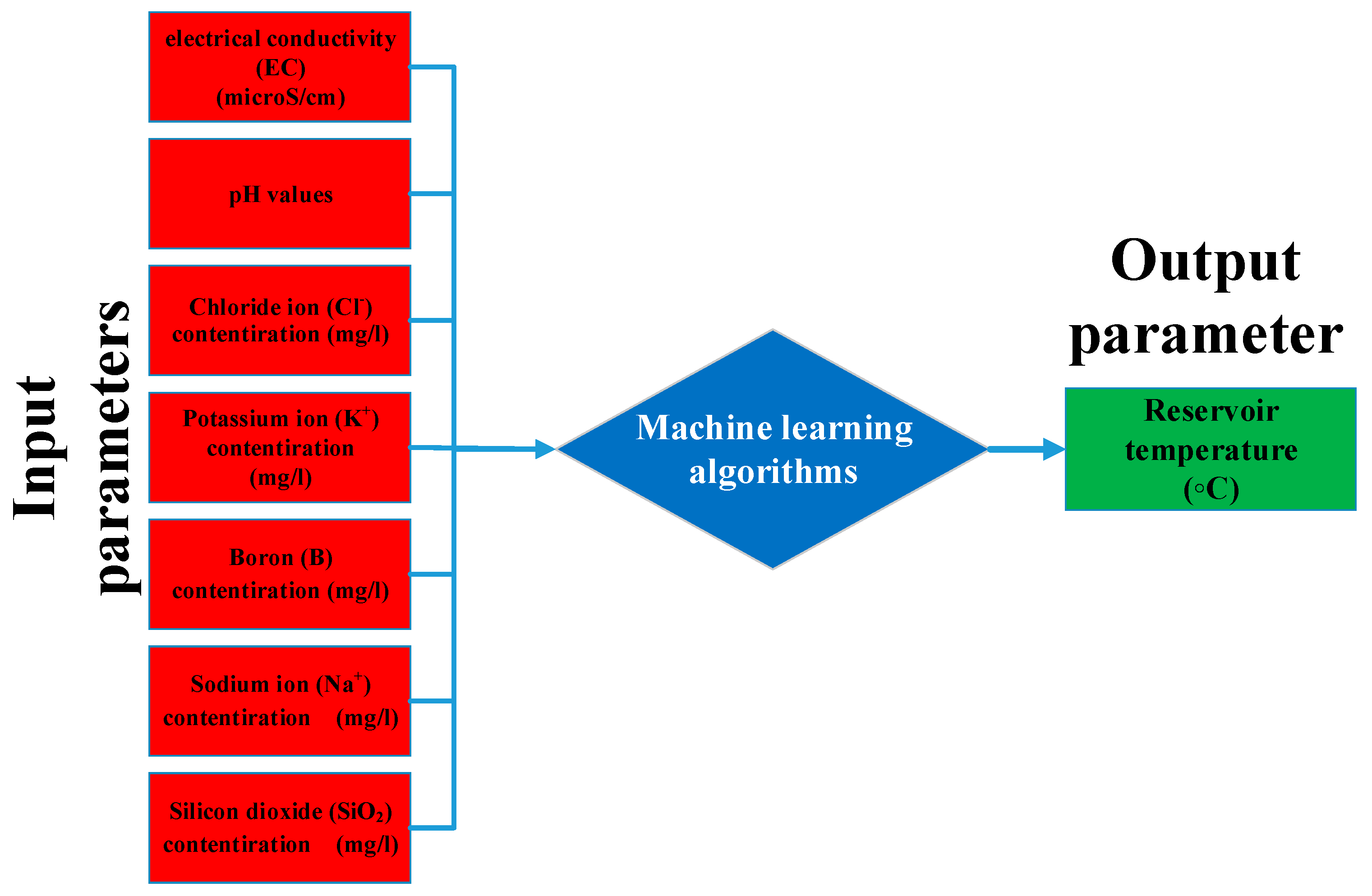
2.1. Data Acquisition

In this study, we utilized a dataset comprising 161 data points, previously assembled by researchers within our team. This dataset, initially used to predict the application areas of reservoir temperatures (RTs) through classification approaches, is the foundation for our current investigation [17]. Herein, we propose a hybrid machine learning approach, the adaptive opposition-based slime mould algorithm–multilayer perceptron (AOSMA-MLP), applied to tackle this real-world problem by predicting the numerical values of RTs—a task commonly addressed with regression techniques in machine learning literature.

To facilitate a comprehensive understanding of the present study, it is pertinent to briefly revisit some critical aspects of the dataset, detailed in our prior research [17]. Figure 1 illustrates the modeling’s input and output parameters, encompassing seven inputs and one output. The selection of ions as input parameters is primarily influenced by their availability in the fluid, given that geothermal fluids, deriving their components from either a degassing magma heat source or the surrounding rock, often contain high concentrations of these ions. Notably, the Na+ and K+ ion concentrations are essential for understanding water–rock interactions at elevated temperatures. Moreover, an increased B content typically signifies deep feeding and a high-temperature deep reservoir. Cl⁻ is a major anion that enhances the salinity of geothermal fluids. The silica concentration, affected by temperature, is another crucial parameter. In a geothermal system, SiO₂’s solubility decreases with falling temperature. Additionally, silica is vital for estimating reservoir temperatures in thermal springs, and its precipitation can influence the operational process. The dissolved ion content in geothermal fluids, indicative of the temperature and reservoir geology of an area, varies with temperature. Low-temperature fluids contain fewer dissolved solids than their high-temperature counterparts, making electrical conductivity (EC) an important measure for assessing dissolved particles in geothermal fluids [12].

This section meticulously details the compilation of a comprehensive dataset utilized in the current study, drawing from various sources focusing on the hydrogeochemical properties and reservoir temperatures (RTs) of geothermal resources across Turkey, particularly within Anatolia. Following is a concise rephrasing to clarify and streamline the information:

The dataset used in this study amalgamates hydrogeochemical data and RTs from several geothermal resources across Western, Central, and Eastern Anatolia, Turkey. It integrates the following.

Western Anatolia: a collection of 83 datasets from [12], detailing hydrogeochemical properties and RTs of geothermal resources. Central Anatolia (Çamlıdere): hydrogeochemical data and RTs sourced from 12 different locations, as reported by [35]. Eastern Anatolia: a selection of 42 datasets from [36], specifically focusing on hot water sources from various cities and locations. Central Anatolia (Nevşehir, Kozaklı): nine datasets from research documented in [37], excluding data from point 4 for consistency. Central Anatolia (Terme and Karakurt, Kırşehir): this study contributed seven datasets, excluding cold spring data but including hydrogeochemical and RT data [38]. Central Anatolia (Seydişehir, Kavak, Konya): eight datasets derived from literature [39], omitting cold spring data but incorporating measurements from April. Each dataset has been meticulously selected to ensure a robust analysis, excluding cold springs, to maintain focus on the geothermal energy potential. The range and specifics of the hydrogeochemical and RT data are tabulated in

Table 1. Range of hydrogeochemical and RT dataset.

	Parameter	Unit	Value
Input Data	pH	-	2.4–9.7
	EC	microS/cm	203–10,434
	K+	mg/L	0.7–191
	Na+		2.6–2600
	Boron		0–38
	SiO2		11–650
	Cl−		2.8–2500
Output Data	RT	°C	11–245

, providing a foundation for the comprehensive analysis undertaken in this study.

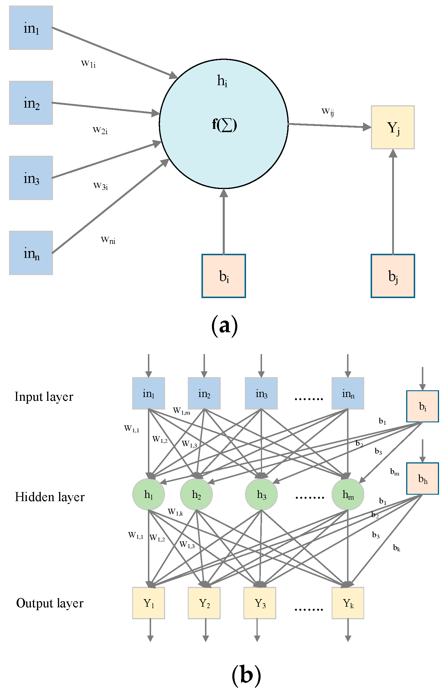
2.2. Artificial Neural Network

The artificial neural network (ANN) is a computational model inspired by the human brain’s neural network. It typically consists of three primary layers: the input layer, one or more hidden layers, and the output layer [40,41]. The primary goal in training an ANN is continuous optimization, which involves mapping input to output to find optimal bias and weight values within the fewest possible iterations. The multilayer perceptron (MLP) is the most frequently utilized ANN structure in the literature. This section delves into MLP and the metaheuristic methods increasingly adopted for MLP training in recent years. Additionally, it covers evaluation metrics for regression problem assessments and data-normalization techniques.

Multi-Layer Perceptron Neural Networks

Similar to ANNs, the MLP functions by mapping a set of input values to a corresponding set of output values. This mapping is achieved through a transformation process designed to derive the output. An MLP consists of three layers: the input layer contains n input values; the hidden layer, positioned between the input and output layers, varies in size depending on the problem type; and the output layer, which aggregates the results of the MLP network [42]. Figure 2a,b illustrate the fundamental MLP structure and a single neuron’s architecture, respectively. The input layer hosts n neurons, the output layer includes k neurons, and the hidden layer comprises m neurons. Each neuron in the hidden layer performs two critical operations: summation and activation. The sum obtained is subsequently passed through an activation function, as depicted in Equation (1).

$${Sum}_j={\sum }_{i=1}^n{w}_{ij}·{in}_i+b_j$$

(1)

where w_ij is the connection weight between the hidden neuron j and the input neuron i. b_j is the bias value.

$${ y}_j=f\left({Sum}_j\right)$$

(2)

where y_j is the output value of neuron j, and f is the sigmoid function. Its calculation is shown in Equation (3).

$$f\left({Sum}_j\right)=\frac{1}{1+e^{{-Sum}_j}}$$

(3)

At the end of these operations, the final output value ${\widehat{\mathit{Y}}}_{\mathit{i}}$ is calculated using the sum and activation operations. These operations are given in Equations (5) and (6).

$${Sum}_j={\sum }_{i=1}^m{w}_{ij}·y_j+b_j$$

(4)

$${\widehat{Y}}_j=f\left({Sum}_j\right)$$

(5)

Here Y_j is the final output of j.

2.3. Whale Optimization Algorithm

Mirjalili and Lewis (2016) introduced the whale optimization algorithm (WOA), a metaheuristic optimization technique inspired by the social behavior of humpback whales specifically designed to tackle challenging optimization problems [43]. Humpback whales are known for their unique hunting strategy, wherein they can pinpoint and entirely engulf their prey. In the context of WOA, this behavior is simulated by allowing the simulated whales to adjust their positions relative to a designated optimal search agent, analogous to the target prey in their natural hunting process. This adaptation of humpback whale behavior into a computational model is encapsulated in the mathematical formulations presented in Equations (6) and (7), detailing the algorithm’s mechanics of search and optimization.

$$\overrightarrow{D}=\left|\overrightarrow{C}.\overrightarrow{X^{\ast }}\left(t\right)-\overrightarrow{\mathrm{X}}\left(t\right)\right|$$

(6)

$$\overrightarrow{X}(t+1)=\overrightarrow{X^{\ast }}\left(t\right)-\overrightarrow{A}.\overrightarrow{D}$$

(7)

The location vector of the optimal solution that has been found up to this point is denoted by $\overrightarrow{{\mathit{X}}^{\ast }}$. $\overrightarrow{\mathit{A}}$ and $\overrightarrow{\mathit{C}}$ coefficient vectors are calculated in Equations (8)–(10). The position vector is denoted by $\overrightarrow{\mathit{X}}$. $\mathit{t}$ represents the most recent iteration.

$$\overrightarrow{A}=2.\overrightarrow{a}.\overrightarrow{r}-\overrightarrow{a}$$

(8)

$$\overrightarrow{a}=2-2\frac{t}{t_{max}}$$

(9)

$$\overrightarrow{C}=2.\overrightarrow{r}$$

(10)

In the whale optimization algorithm (WOA), a coefficient vector “a” decreases linearly from 2 to 0 over the course of iterations, influencing both the exploration and exploitation phases. The vector “r” is a randomly generated vector within the range of [0, 1], with “t_max” representing the maximum number of iterations and “t” denoting the current iteration number. Equations (8) and (9) are designed to maintain a balance between exploration and exploitation during the optimization process. In these equations, “r” generates a random number, introducing stochastic elements into the population’s location updates. Exploration is initiated when A ≥ 1, while exploitation occurs when A < 1, enabling the algorithm to transition between exploration and exploitation at any optimization stage.

The unique bubble-net attacking strategy of humpback whales is mimicked within WOA through two main mechanisms: the spiral update position mechanism and the shrinking encircling mechanism. The coefficient vector A, which influences these mechanisms, is determined by setting the value of “a” within the range of [−1, 1] [−1, 1], while the shrinking encircling mechanism reduces the value of “a” linearly through iterations. This approach positions the new location midway between its current location and that of the optimal search agent. To emulate the humpback whales’ spiral movements toward their prey, the spiral equation defining the path between the whale and the prey’s location is established. This mathematical representation captures the essence of the humpback whales’ hunting strategy, applying it to the optimization process in WOA

$$\overrightarrow{X}\left(t+1\right)=\overrightarrow{D^{\mathrm{\prime }}}.e^{bl}.\cos \left(2\pi l\right)+\overrightarrow{X^{\ast }}\left(t\right)$$

(11)

$$\overrightarrow{D^{\mathrm{\prime }}}=\left|\overrightarrow{X^{\ast }}\left(t\right)-\overrightarrow{\mathrm{X}}\left(t\right)\right|$$

(12)

where $\overrightarrow{{\mathit{D}}^{\mathbf{\prime }}}$ is the distance of the $\mathit{i}$ whale from its target (the best solution so far), $\mathit{l}$ is a random value within the range $[-1, 1]$, and $\mathit{b}$ is a constant used to define the logarithmic spiral’s form. Because humpback whales swim in a circle that gets smaller and smaller around their prey while at the same time moving along the path in a spiraling fashion, the shrinking containment method and the spiral approach are used simultaneously. In order to model this behavior, it is presumed that each mechanism has a probability of occurring of fifty percent [44]. The method based on the variation of vector A can be utilized for hunting (exploration). Random searches are conducted by humpback whales based on one another’s locations. As a result, A is used in conjunction with random values less than or greater than 1 to force the search agent to depart from the reference whale. During the exploration phase, in contrast to the exploitation phase, they do not update the position of a search agent according to the best search agent discovered up to this point. Instead, they choose a search agent at random and base the update on that. This mechanism highlights the A > 1 discovery phase and allows WOA to conduct a global search. Equations (13) and (14) are a mathematical model of the process of hunting prey.

$$\overrightarrow{D}=\left|\overrightarrow{C}.\overrightarrow{X_{rand}}-\overrightarrow{\mathrm{X}}\right|$$

(13)

$$\overrightarrow{X}\left(t+1\right)=\overrightarrow{X_{rand}}-\overrightarrow{A}.\overrightarrow{D}$$

(14)

where $\overrightarrow{X_{rand}}$ is a randomly selected whale from the current population whose position vector is random.

2.4. Ant Lion Algorithm

The ant lion optimizer (ALO) algorithm models the interaction between ant lions and ants within the context of a trap [45]. In this algorithm, ant lions set traps to capture ants, thereby enhancing their fitness through successful predation. Ants, symbolizing potential solutions within the search space, navigate through this space to mirror these natural interactions. Reflecting the stochastic movement of ants in their quest for food, the algorithm employs a specific random walk strategy to simulate the ants’ movement patterns. This approach captures the essence of the dynamic and unpredictable interactions that occur in nature, translating them into a computational method for solving optimization problems.

$$X\left(t\right)=[0, cumsum\left(2r\left(t_1\right)-1\right), cumsum\left(2r\left(t_2\right)-1,\dots , cumsum\left(2r\left(t_n\right)-1\right)\right)],$$

(15)

where cumsum is a function that calculates the cumulative sum, n is the maximum number of iterations that may occur, t represents the step of a random walk (referred to as an iteration in this research), and r(t) is a stochastic function defined as follows:

$$r\left(t\right)=\left\{\begin{array}{c}1, if rand>0.5\\ 0, if rand\le 0.5\end{array}\right.$$

(16)

where rand is a uniformly distributed random number in the range [0, 1]. In the following matrix, the ant’s location is noted and used for optimization:

$$M_{ant}=\left[\genfrac{}{}{0pt}{}{A_{\mathrm{1,1}} A_{\mathrm{1,2}} \dots \dots A_{1,d}}{\begin{array}{c}{A}_{\mathrm{2,1}} A_{\mathrm{2,2}} \dots \dots A_{2,d}\\ .\\ .\\ A_{n,1} A_{n,2} \dots \dots A_{n,d}\end{array}}\right]$$

(17)

where ${\mathit{M}}_{\mathit{a}\mathit{n}\mathit{t}}$ stores the location of each ant, ${\mathit{A}}_{\mathit{i},\mathit{j}}$ indicates the $\mathit{i}$th ant’s $\mathit{j}$th variable (dimension), $\mathit{d}$ is the number of variables, and $\mathit{n}$ is the number of ants. During optimization, a fitness (objective) function is used to assess each ant, and the fitness value of each ant is stored in the following matrix:

$$M_{OA}=\left[\genfrac{}{}{0pt}{}{{f\left(\right[A}_{\mathrm{1,1}} A_{\mathrm{1,2}} \dots \dots A_{1,d}\left]\right)}{\begin{array}{c}{f\left(\right[A}_{\mathrm{2,1}} A_{\mathrm{2,2}} \dots \dots A_{2,d}\left]\right)\\ .\\ .\\ {f\left(\right[A}_{n,1} A_{n,2} \dots \dots A_{n,d}\left]\right)\end{array}}\right]$$

(18)

where ${\mathit{M}}_{\mathit{O}\mathit{A}}$ is the matrix used for preserving each ant’s fitness, and $\mathit{f}$ is the fitness (objective) function. In addition, the ant lions lurk in the search area. Their locations are saved using the following matrices:

$$M_{Antlion}=\left[\genfrac{}{}{0pt}{}{{AL}_{\mathrm{1,1}} {AL}_{\mathrm{1,2}} \dots \dots {AL}_{1,d}}{\begin{array}{c}{AL}_{\mathrm{2,1}} {AL}_{\mathrm{2,2}} \dots \dots {AL}_{2,d}\\ .\\ .\\ {AL}_{n,1} {AL}_{n,2} \dots \dots {AL}_{n,d}\end{array}}\right]$$

(19)

M_Antlion is the matrix used to store each ant lion’s location.

$$M_{OAL}=\left[\genfrac{}{}{0pt}{}{{f\left(\right[AL}_{\mathrm{1,1}} {AL}_{\mathrm{1,2}} \dots \dots {AL}_{1,d}\left]\right)}{\begin{array}{c}{f\left(\right[AL}_{\mathrm{2,1}} {AL}_{\mathrm{2,2}} \dots \dots {AL}_{2,d}\left]\right)\\ .\\ .\\ {f\left(\right[AL}_{n,1} {AL}_{n,2} \dots \dots {AL}_{n,d}\left]\right)\end{array}}\right]$$

(20)

M_OAL is the matrix used to save each ant lion’s fitness.

2.4.1. Random Walks of Ants

Equation (21) is used to normalize ants’ positions and restrict them from wandering outside of the search area.

$$X_i^t=\frac{{(X}_i^t-a_i)-(d_i-c_i^t)}{d_i^t-a_i}+c_i$$

(21)

where ${\mathit{a}}_{\mathit{i}}$ denotes the smallest random walk for the $\mathit{i}$th variable, ${\mathit{c}}_{\mathit{i}}^{\mathit{t}}$ denotes the smallest variable at the $\mathit{t}$th iteration, and ${\mathit{d}}_{\mathit{i}}^{\mathit{t}}$ represents the largest variable at the $\mathit{t}$th iteration.

2.4.2. Trapping in Antlion’s Pits

Ant lion traps affect random ant walks. The following equations are proposed to describe this supposition:

$$c_i^t={Antlion}_j^t+c^t$$

(22)

$$d_i^t={Antlion}_j^t+d^t$$

(23)

where ${\mathit{c}}^{\mathit{t}}$ stands for the vector containing all variables’ minimum values at iteration $\mathit{t}$; ${\mathit{d}}^{\mathit{t}}$ stands for the vector containing all variables’ maximum values at iteration $\mathit{t}$; ${\mathit{c}}_{\mathit{i}}^{\mathit{t}}$ and ${\mathit{d}}_{\mathit{i}}^{\mathit{t}}$ represent the minimum and maximum values of all variables for the $\mathit{i}$-th ant, respectively; and ${\mathit{A}\mathit{n}\mathit{t}\mathit{l}\mathit{i}\mathit{o}\mathit{n}}_{\mathit{j}}^{\mathit{t}}$ represents the position of the selected $\mathit{j}$-th.

2.4.3. Building Trap

The capacity of ant lions to hunt should be modeled using a selection method. The more fit the ant lion, the greater its chance of catching an ant. The roulette wheel selection method was used to choose ant lions based on their fitness value.

2.4.4. Sliding Ants towards Antlion

Ants must walk in a random pattern, while ant lions can construct traps according to their fitness. Antlions spray sand from the pit once an ant is inside the trap. This behavior hinders an ant’s escape. In order to show this behavior, the size of the ants’ random walk’s hypersphere is made smaller. In this respect, the following equations are suggested:

$$c^t=\frac{c^t}{l}$$

(24)

$$d^t=\frac{d^t}{l}$$

(25)

where ${\mathit{c}}^{\mathit{t}}$ represents the lowest value for all variables at iteration $\mathit{t}$, ${\mathit{d}}^{\mathit{t}}$ is the vector containing $\mathit{t}$s’ maximum value for all variables, and $\mathit{I}$ is a ratio, as described by Equation (26).

$$l={10}^w\frac{t}{t_{max}}$$

(26)

where $\mathit{w}$ is a constant determined depending on the current iteration ($\mathit{w}=\mathbf{2}$ when $\mathit{t}>\mathbf{0.1}{\mathit{t}}_{\mathit{m}\mathit{a}\mathit{x}}$, $\mathit{w}=\mathbf{3}$ when $\mathit{t}>\mathbf{0.5}{\mathit{t}}_{\mathit{m}\mathit{a}\mathit{x}}$, $\mathit{w}=\mathbf{4}$ when $\mathit{t}>\mathbf{0.75}{\mathit{t}}_{\mathit{m}\mathit{a}\mathit{x}}$, $\mathit{w}=\mathbf{5}$ when $\mathit{t}>\mathbf{0.9}{\mathit{t}}_{\mathit{m}\mathit{a}\mathit{x}}$, and $\mathit{w}=\mathbf{6}$ when $\mathit{t}>\mathbf{0.95}{\mathit{t}}_{\mathit{m}\mathit{a}\mathit{x}}$), where $\mathit{t}$ is the current iteration, and ${\mathit{t}}_{\mathit{m}\mathit{a}\mathit{x}}$ is the maximum number of iterations. In essence, the constant $\mathit{w}$ allows for exploitation accuracy level adjustment.

2.4.5. Sliding Ants towards Antlion

The prey is captured by the ant lion’s jaws as it descends to the bottom of the pit during the last phase of the hunt. The ant lion then drags the ant into the sand, where it eats the insect’s body. When an ant becomes more physically fit than its comparable ant lion, it is considered that prey is captured. In order to expand its capacity for hunting fresh ants, the ant lion must thus change its posture to that of the hunted ant. Equation (27) represents this process:

$${Antlion}_j^t={Ant}_i^t if f\left({Ant}_i^t\right)>f\left({Antlion}_j^t\right)$$

(27)

where ${\mathit{A}\mathit{n}\mathit{t}\mathit{l}\mathit{i}\mathit{o}\mathit{n}}_{\mathit{j}}^{\mathit{t}}$ displays the position of chosen $\mathit{j}$-th antlion at the $\mathit{t}$-th iteration, and ${\mathit{A}\mathit{n}\mathit{t}}_{\mathit{i}}^{\mathit{t}}$ shows the position of the $\mathit{i}$-th ant at the $\mathit{t}$-th iteration.

2.4.6. Elitism

The ant lion that is fittest in each iteration is labeled an elite. The chosen ant lion and the elite ant lion direct the random walk of an ant using the selection process, and so the repositioning of a particular ant follows Equation (28).

$${Ant}_i^t=\frac{R_A^t+R_E^t}{2}$$

(28)

where ${\mathit{A}\mathit{n}\mathit{t}}_{\mathit{i}}^{\mathit{t}}$ denotes the location of the $\mathit{i}$-th ant at the $\mathit{t}$-th iteration, ${\mathit{R}}_{\mathit{A}}^{\mathit{t}}$ denotes the $\mathit{t}$-th iteration’s random walk around the ant lion chosen by the roulette wheel, and ${\mathit{R}}_{\mathit{E}}^{\mathit{t}}$ denotes the $\mathit{t}$-th iteration’s random walk around the elite.

2.5. Slime Mould Algorithm and Adaptive Opposition Slime Mould Algorithm

A stochastic optimizer called SMA has been proposed by Li et al. [46]. Inspired by the oscillation of the mode of slime mould in nature, the proposed SMA method has been successfully applied in many studies in the literature [47,48]. Suppose there are $\mathit{N}$ slime moulds with a lower boundary ($\mathit{L}\mathit{B}$) and upper boundary ($\mathit{U}\mathit{B}$) in the search space. The position of the $\mathit{i}$th slime mould in $\mathit{d}$ dimensions is represented as ${\mathit{X}}_{\mathit{i}}=\left({\mathit{x}}_{\mathit{i}}^{\mathbf{1}},{\mathit{x}}_{\mathit{i}}^{\mathbf{2}},\dots ,{\mathit{x}}_{\mathit{i}}^{\mathit{d}}\right),\forall \mathit{i}\in [\mathbf{1},\mathit{N}]$, and the fitness of $\mathit{i}$-th slime is expressed as $\mathit{f}\left({\mathit{X}}_{\mathit{i}}\right),\forall \mathit{i}=[\mathbf{1},\mathit{N}]$. Thus, the position of $\mathit{N}$ slime mould and its fitness at the present moment (iteration) $\mathit{t}$ may be stated according to Equations (29) and (30):

$$X\left(t\right)=\left[\begin{array}{c}{x}_1^1 x_1^2 \cdots x_1^d\\ x_2^1 x_2^2 \cdots x_2^d\\ ⋮ ⋮ ⋮ ⋮\\ x_N^1{x}_N^2 \cdots x_N^d\end{array}\right]=\left[\begin{array}{c}{X}_1\\ X_2\\ ⋮\\ X_N\end{array}\right]$$

(29)

$$f\left(X\right)=\left[f\left(X_1\right), f\left(X_2\right),\dots ,f\left(X_N\right)\right]$$

(30)

For the next iteration ($\mathit{t}+\mathbf{1}$) in the SMA, the position of the slime mould is updated using Equation (31).

$${\mathit{X}}_{\mathit{i}}\left(\mathit{t}+\mathbf{1}\right)=\left\{\begin{array}{c}{\mathit{X}}_{\mathit{L}\mathit{B}}\left(\mathit{t}\right)+{\mathit{V}}_{\mathit{b}}\left(\mathit{W}·{\mathit{X}}_{\mathit{A}}\left(\mathit{t}\right)-{\mathit{X}}_{\mathit{B}}\left(\mathit{t}\right)\right) {\mathit{r}}_{\mathbf{1}}\ge \mathit{\delta } \mathit{a}\mathit{n}\mathit{d} {\mathit{r}}_{\mathbf{2}}<{\mathit{p}}_{\mathit{i}}\\ {\mathit{V}}_{\mathit{c}}·{\mathit{X}}_{\mathit{i}}\left(\mathit{t}\right) { \mathit{r}}_{\mathbf{1}}\ge \mathit{\delta } \mathit{a}\mathit{n}\mathit{d} {\mathit{r}}_{\mathbf{2}}\ge {\mathit{p}}_{\mathit{i}}\\ \mathit{r}\mathit{a}\mathit{n}\mathit{d} ·\left(\mathit{U}\mathit{B}-\mathit{L}\mathit{B}\right)+\mathit{L}\mathit{B} {\mathit{r}}_{\mathbf{1}}<\mathit{\delta }\end{array}, \forall \mathit{i}\in [\mathbf{1},\mathit{N}]\right.$$

(31)

where ${\mathit{V}}_{\mathit{b}}$ and ${\mathit{V}}_{\mathit{c}}$ represent random velocity, ${\mathit{X}}_{\mathit{L}\mathit{B}}$ represents the best local individual for the current iteration, $\mathit{W}$ represents the weight vector, and ${\mathit{X}}_{\mathit{A}}$ and ${\mathit{X}}_{\mathit{B}}$ represent randomly pooled slime mould samples from the available populations. ${\mathit{r}}_{\mathbf{1}}$ and ${\mathit{r}}_{\mathbf{2}}$ are random values between 0 and 1. The probability that the slime mould will appear at a random search site is set at $\mathit{\delta }$ 0.03. ${\mathit{p}}_{\mathit{i}}$ is the $\mathit{i}$-th slime mould’s threshold value, which assists in picking the slime mould position using the best individual or itself for the following iteration, and is computed as shown in Equation (32).

$$p_i=\tan h\left|f\left(X_i\right)-f_{GB}\right|,\forall i\in [1,N],$$

(32)

where $\mathit{f}\left({\mathit{X}}_{\mathit{i}}\right)$ is the fitness value of the $\mathit{i}$-th slime mould ${\mathit{X}}_{\mathit{i}},$ and $\mathit{f}\left({\mathit{X}}_{\mathit{G}\mathit{B}}\right)$ is the global best fitness value ${\mathit{f}}_{\mathit{G}\mathit{B}}$ derived by Equation (33) of the global best position ${\mathit{X}}_{\mathit{G}\mathit{B}}$.

$$f_{GB}=f\left(X_{GB}\right)$$

(33)

Equation (34) may be used to calculate the weight $\mathit{W}$ of $\mathit{N}$ different types of slime mould in the current iteration:

$$W\left({sortInd}_f\left(i\right)\right)=\left\{\begin{array}{c}1+rand ·\log \left(\frac{f_{LB}-f\left(X_i\right)}{f_{LB}-f_{LW}}+1\right) 1\le i\le \frac{N}{2}\\ 1-rand·\log \left(\frac{f_{LB}-f\left(X_i\right)}{f_{LB}-f_{LW}}+1\right) \frac{N}{2}<i\le N\end{array}\right.$$

(34)

where “rand” represents a random number between [0, 1]. The local worst fitness value is represented by ${\mathit{f}}_{\mathit{L}\mathit{w}}$, and the local best fitness value is represented by ${\mathit{f}}_{\mathit{L}\mathit{B}}$. ${\mathit{f}}_{\mathit{L}\mathit{B}}$ and ${\mathit{f}}_{\mathit{L}\mathit{w}}$ are calculated based on the fitness value $\mathit{f}$ given in Equation (30). We can sort the fitness value in ascending order for a minimization problem, as shown in Equation (35):

$$\left[{Sort}_f,{SortInd}_f\right]=sort\left(f\right)$$

(35)

The local worst fitness value Equation (36), the local best fitness value Equation (37), and the corresponding local best individual value Equation (38) are subtracted as follows:

$$f_{Lw}=f\left({Sort}_f\left(N\right)\right)$$

(36)

$$f_{LB}=f\left({Sort}_f\right(1\left)\right)$$

(37)

$${ X}_{LB}=X\left({SortInd}_f\right(1\left)\right)$$

(38)

where ${\mathit{V}}_{\mathit{b}}$ and ${\mathit{V}}_{\mathit{c}}$ represent random velocities selected from a continuous uniform distribution in the $[-\mathit{b},\mathit{b}]$ range and in the $[-\mathit{c},\mathit{c}]$ range. The $\mathit{b}$ and $\mathit{c}$ values for the $\mathit{t}$ iteration are calculated as shown in Equations (39) and (40):

$$b=\arctan h(-\left(\frac{t}{T}.\right)+1)$$

(39)

$$c=1-\frac{t}{T}$$

(40)

The ideal feeding path for slime mould may be improved in the search process, as explained in Equation (31) [34]. Based on $\mathit{\delta }$ and ${\mathit{p}}_{\mathit{i}}$, the next iteration position update rule of slime mould in SMA is dependent on the following three cases:

Case 1: When ${\mathit{r}}_{\mathbf{1}}\ge \mathit{\delta } \mathrm{a}\mathrm{n}\mathrm{d} {\mathit{r}}_{\mathbf{2}}<{\mathit{p}}_{\mathit{i}}$, the slime mould search trajectory is directed by the best local slime ${\mathit{X}}_{\mathit{L}\mathit{B}}$ and two randomly pooled slimes ${\mathit{X}}_{\mathit{A}}$ and ${\mathit{X}}_{\mathit{B}}$ with the velocity ${\mathit{V}}_{\mathit{b}}$. It balances exploration and exploitation. Case 1 indicates that ${\mathit{X}}_{\mathit{A}}$ and ${\mathit{X}}_{\mathit{B}}$ are arbitrarily combined slime mould; therefore, the solutions we acquire are not well explored and exploited [34]. This limitation may be solved by substituting ${\mathit{X}}_{\mathit{A}}$ with the best local ${\mathit{X}}_{\mathit{L}\mathit{B}}$. In this case, the equation can be updated, as shown in Equation (41).

$$\begin{gathered} {Xn}_i\left(t\right)=X_{LB}\left(t\right)+V_b\left(W·X_{LB}\left(t\right)-X_B\left(t\right)\right), if r_1\ge \delta and r_2<p_i \\ {Xn}_i\left(t\right)=V_c·X_i\left(t\right), if r_1\ge \delta and r_2\ge p_i \\ {Xn}_i\left(t\right)=rand·\left(UB-LB\right)+LB, if r_1<\delta \end{gathered}$$

(41)

Case 2: The slime mould trajectory is directed by its own location with a velocity ${\mathit{V}}_{\mathit{c}}$ when ${\mathit{r}}_{\mathbf{1}}\ge \mathit{\delta } \mathrm{a}\mathrm{n}\mathrm{d} {\mathit{r}}_{\mathbf{2}}\ge {\mathit{p}}_{\mathit{i}}$. This helps with exploitation. According to Case 2, the slime mould utilizes a neighboring location; thus, it may take a different route with a lower fitness value. An adaptive decision (AD) strategy might be a better option to overcome this limitation [34].

Case 3: When ${\mathit{r}}_{\mathbf{1}}<\mathit{\delta }$, in the search space, the slime mould re-initializes, assisting with exploration. Based on Case 3, the SMA provides a provision for devoted exploration; nevertheless, the exploration is limited since $\mathit{\delta }$ has a small value. We must add more exploration to SMA in order to assist it in circumventing this limitation and exceeding the local minima. To address the limitations of Cases 2 and 3, we employ an AD technique to determine if it is necessary to investigate further using OBL [34].

2.5.1. Opposition-Based Learning

The OBL updated the location of the subsequent iterations by comparing an estimate ${\mathit{X}\mathit{o}}_{\mathit{i}}$ in the search space that is the exact opposite of the position ${\mathit{X}\mathit{n}}_{\mathit{i}}$ for each slime mould ($\mathit{i}=\mathbf{1},\mathbf{2},\dots ,\mathit{N}$). With increased convergence, this step reduces the likelihood of being stranded in the local minima. Thus, it is calculated that the ${\mathit{X}\mathit{o}}_{\mathit{i}}$ for the $\mathit{i}$-th slime mould in the $\mathit{j}$-th dimension is,

$${Xo}_i^j\left(t\right)=\mathit{min}\left({Xn}_i\left(t\right)\right)+\mathit{max}\left({Xn}_i\left(t\right)\right)-{Xn}_i^t\left(t\right)$$

(42)

where $\mathit{i}=\mathbf{1},\mathbf{2},\dots ,\mathit{N}$ and $\mathit{j}=\mathbf{1},\mathbf{2},\dots ,\mathit{d}$. $\mathit{i}$ is chosen for the ${\mathit{X}\mathit{s}}_{\mathit{i}}$ minimization problem. The slime mould position is as follows:

$${Xs}_i\left(t\right)=\left\{\begin{array}{c}{Xo}_i\left(t\right) if f\left({Xo}_i\left(t\right)\right)<f\left({Xn}_i\left(t\right)\right)\\ {Xn}_i\left(t\right) if f\left({Xo}_i\left(t\right)\right)\ge f\left({Xn}_i\left(t\right)\right)\end{array}\right.$$

(43)

2.5.2. Adaptive Decision Strategy

An AD is made based on the present fitness value of $\mathit{f}\left({\mathit{X}\mathit{n}}_{\mathit{i}}\left(\mathit{t}\right)\right)$ and the old fitness value of $\mathit{f}\left({\mathit{X}}_{\mathit{i}}\left(\mathit{t}\right)\right)$ while the slime mould is pursuing a decedent nutrition route. When necessary, the AD uses OBL to augment the investigation. The AD method of AOSMA is then used to adjust the location for the next iteration and is depicted as shown in Equation (44).

$$X_i\left(t+1\right)=\left\{\begin{array}{c}{Xn}_i\left(t\right) if f\left({Xn}_i\left(t\right)\right)\le f\left(X_i\left(t\right)\right)\\ {Xs}_i\left(t\right) if f\left({Xn}_i\left(t\right)\right)>X_i\left(t\right)\end{array}, \forall i\in [1,N]\right.$$

(44)

Surprisingly, the suggested AOSMA improves the efficiency of SMA by using an AD technique to determine if OBL is required along the search trajectory.

2.6. Metaheuristic Optimization Algorithms for Learning Mlp

In the literature, many metaheuristic methods have been proposed to develop the MLP network in the training phase. SMA, ALO, WOA and AOSMA metaheuristic methods are among those that are widely used with success. The successful application of these methods to benchmark functions and real-world problems in the literature has motivated the selection of the methods. In the training phase of MLP, metaheuristic optimization methods are used to determine the bias and weight values that make up the network connections. Four methods are used to find the optimal set of bias and weight values. There is no accepted equation in the literature for selecting the number of hidden nodes. In this study, it was obtained using the following equation:

$$m=2·d+1$$

(45)

Here, $\mathit{d}$ is the number of data features, and $\mathit{m}$ is the number of neurons. The $\mathit{n}$ value, that is, the total weight and bias value, was calculated using the equation below.

$$n=\left(d·m\right)+\left(2·m\right)+1$$

(46)

Search agents commonly found in metaheuristic optimization methods represent a vector with $\mathit{n}$ floating-point numbers. The flow chart of the proposed methods is demonstrated in Figure 3. The use of metaheuristic methods in the training phase of MLP generally covers four processes. First, initialization is initiated by specifying the MLP structure, such as the number of neurons $\left(\mathit{m}\right)$ and the total weight and bias values $\left(\mathit{n}\right)$. Then, the MLP network set—that is, the bias and weight values—are randomly generated. Then, the second step, the fitness evaluation step, is passed. In this step, the fitness value is calculated. For the fitness value, the fitness function must be selected. In this study, the MSE value was chosen, and its equation is given below.

$$\mathrm{M}\mathrm{S}\mathrm{E}=\frac{1}{k}{\sum }_{i=1}^k{(Y_i-{\widehat{Y}}_i)}^2$$

(47)

Here, ${\widehat{\mathit{y}}}_{\mathit{i}}$ is the predictive value, ${\mathit{y}}_{\mathit{i}}$ is the actual value, and $\mathit{k}$ is the number of samples in the training set. In the third step, the update step, the best global fitness value, and personal fitness values are updated for each search agent. Finally, there is the termination step. The termination step is used to continue training the MLP until the maximum number of iterations is achieved.

2.7. Evaluation Metrics

Four different evaluation metrics, namely, R², R, RMSE, and MAE, were used in this study. These metrics are widely used in the literature to compare the performances of the models proposed for predicting regression problems [40,49]. Equations of evaluation metrics are given in Equations (48)–(51).

$$R^2=1-\left(\frac{\sum _j{\left(Y_j-{\widehat{Y}}_j\right)}^2}{\sum _j{(Y_j-\widehat{Y})}^2}\right)$$

(48)

$$p\left(Y,\widehat{Y}\right)=\frac{1}{n-1}{\sum }_{j=1}^n\left(\frac{Y_j-{\mu }_Y}{{\sigma }_Y}\right)\left(\frac{{\widehat{Y}}_j-{\mu }_{\widehat{Y}}}{{\sigma }_{\widehat{Y}}}\right)$$

(49)

$$\mathrm{R}\mathrm{M}\mathrm{S}\mathrm{E}=\sqrt{\left(\frac{1}{n}\right)\times {\sum }_j{\left|Y_j-{\widehat{Y}}_j\right|}^2}$$

(50)

$$\mathrm{M}\mathrm{A}\mathrm{E}=\frac{1}{n}{\sum }_{j=1}^n\left|Y_j-{\widehat{Y}}_j\right|$$

(51)

2.8. Normalization

In this study, min-max [0, 1] normalization was applied to the dataset. The min-max normalization equation is given in Equation (52).

$$min-max; x_{i,n}^{\prime }=\frac{x_{i,n}-{min(x}_i)}{{max(x}_i)-{min(x}_i)}$$

(52)

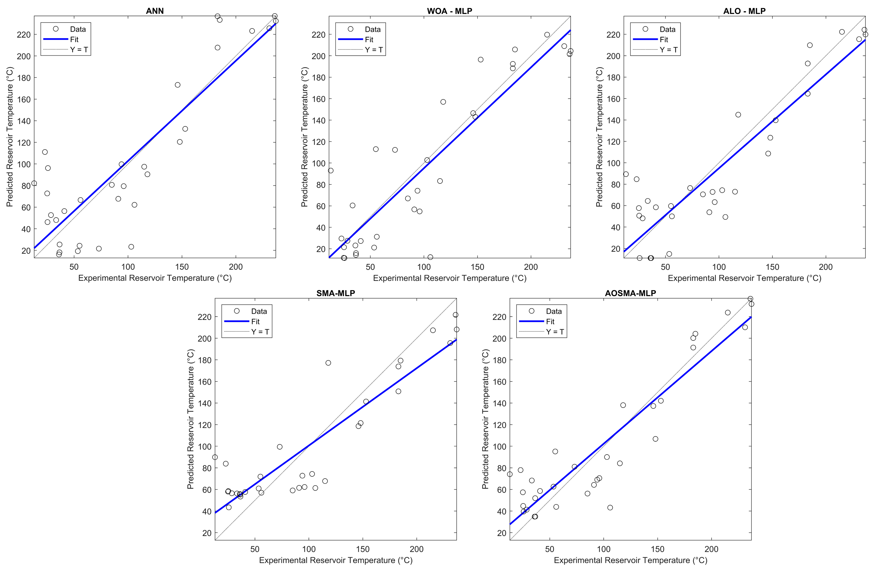
3. Results

In this study, the reservoir temperature (RT) was predicted using several approaches: an MLP trained with a classical optimization method, MLPs trained with three distinct metaheuristic methods, and the AOSMA-MLP, which was proposed for the first time. The dataset comprised 161 samples, encompassing hydrogeochemical data and RTs from geothermal resources across various regions in Anatolia, Turkey. Understanding RTs is essential for determining the most effective use of geothermal resources, whether for direct heating applications or electricity generation, depending on the RT. The dataset was divided into training and test sets, constituting 80% (128 samples) and 20% (33 samples) of the data, respectively. This division ensured consistency across the four models proposed in the study. The metaheuristic methods employed were the whale optimization algorithm (WOA), ant lion optimizer (ALO), slime mould algorithm (SMA), and the newly proposed adaptive opposition-based slime mould algorithm (AOSMA). Characteristics of the MLPs trained using these metaheuristic optimization methods are detailed in

Table 2. Properties of the MLP.

NA	NS	NTRS	NTS	HNO	Dim	W	B	NNS
7	161	128	33	15	136	120	16	7-15-1

, including the number of hidden neurons (HNO), which was kept consistent across all models. For the classical optimization-based training of MLP, the one-step secant backpropagation method was utilized. Table 2 outlines various parameters, including the number of attributes (NA), samples (NS), training samples (NTRS), test samples (NTS), hidden neurons (HNO), dimension (Dim), weight (W), bias (B), and neural network structure (NNS). Additionally,

Table 3. The parameters of the metaheuristic optimization methods.

Algorithm	Parameters	Values
WOA	$\overrightarrow{a}$ Shape of the logarithmic spiral ($b$)	Linearly decreased from 2 to 0 1
SMA	$\delta$	0.03
AOSMA	$\delta$	0.03

lists the parameters of the employed metaheuristic optimization methods, with the maximum number of iterations and the number of search agents standardized at 200 and 30, respectively, to facilitate equal evaluation conditions across all methods.

The training durations for the metaheuristic optimization methods, namely, ALO-MLP, WOA-MLP, SMA-MLP, and AOSMA-MLP, were recorded as 13.07, 8.06, 8.17, and 8.26 min, respectively, highlighting the efficiency and potential applicability of these advanced computational techniques in geothermal resource evaluation.

4. Discussion

To assess the effectiveness of the models proposed in this study, four widely recognized evaluation metrics were employed: R-squared (R²), correlation coefficient (R), root mean square error (RMSE), and mean absolute error (MAE). The comparative results of the four models are systematically presented in

Table 4. Performance of ANN, ALO-MLP, WOA-MLP, SMA-MLP, and AOSMA-MLP on hydrogeochemical and RT data.

	R2	R	RMSE	MAE
ANN	0.7169	0.8701	36.94	29.28
WOA-MLP	0.7765	0.8969	32.82	25.26
ALO-MLP	0.8096	0.9049	30.29	25.67
SMA-MLP	0.7955	0.8974	31.39	26.81
AOSMA-MLP	0.8514	0.9233	26.76	21.45

, with the most favorable outcomes highlighted for clarity.

A detailed analysis revealed the following insights based on the evaluation metrics:

• R² Value: The AOSMA-MLP algorithm outperformed the ANN, WOA-MLP, ALO-MLP, and SMA-MLP methods by 18.76%, 9.65%, 5.16%, and 7.03%, respectively, indicating a more accurate fit to the data.
• R Value: In terms of correlation, the AOSMA-MLP method exhibited superior performance by 6.11%, 2.94%, 2.03%, and 2.89% compared to the ANN, WOA-MLP, ALO-MLP, and SMA-MLP algorithms, respectively, suggesting stronger linear relationships between predicted and observed values.
• RMSE Value: The AOSMA-MLP model demonstrated a significant reduction in prediction error, showing improvements of 27.56%, 18.46%, 11.65%, and 14.75% over the ANN, WOA-MLP, ALO-MLP, and SMA-MLP algorithms, respectively.
• MAE: In terms of absolute errors, the AOSMA-MLP approach was found to be more precise, reducing errors by 26.74%, 15.08%, 16.44%, and 19.99% compared to the ANN, WOA-MLP, ALO-MLP, and SMA-MLP algorithms, respectively.

Upon a comprehensive review of Table 4, the AOSMA-MLP model surpasses its counterparts across all evaluated metrics, establishing its superiority and effectiveness in predicting the reservoir temperatures (RTs) of geothermal resources. This comparative analysis underscores the potential of the AOSMA-MLP approach as a more accurate and reliable method for RT prediction in geothermal studies. In the study conducted by Tut Hakkidir, the RT value was predicted using linear regression, a linear support vector machine, and a deep neural network (DNN). A total of 83 different datasets were used in the study, and the best result was obtained in DNN. DNN achieved an MAE value of 6.45 and an RMSE value of 8.29 [12]. In the study conducted by Bemah et al., the RT value was estimated using natural gradient boosting (NGB), extreme learning machine, group method of data handling, generalized regression neural network, and back propagation neural network methods. A total of 83 different datasets were used in the study, and the best result was obtained with the NGB method. The NGB MAE was calculated at 3.97, RMSE at 4.59, and R² at 0.9959 [50]. In another study by Quan et al., the RT value was estimated using ANN, support vector regression genetic algorithm SVR, and improved support vector machine (M-GASVR) methods. The M-GASVR method yielded the best results in the study. The M-GASVR was calculated as MAE 0.45, RMSE 0.556, and R² 0.903 [51]. Perez-Zarate and colleagues conducted a study using different ANN models to predict the RT value. In the study, the ANN model that gave the best results was calculated as MAE 18.32, RMSE 26.4971, and R 0.7165 [24].

Figure 4 compares predicted and actual reservoir temperatures (RTs) using four distinct models. Figure 4 shows that the multilayer perceptron (MLP) trained via the adaptive opposition-based slime mould algorithm (AOSMA) yields predictions that are significantly closer to actual values compared to other models. Notably, at index numbers 1, 15, 17, and 28, AOSMA-MLP demonstrates remarkable accuracy, predicting values that closely mirror the true RTs.

Further insight is provided by scatter plots depicted in Figure 5. This graphical representation reinforces the accuracy of AOSMA-MLP, showcasing its predictions in close alignment with real RT values. The scatter plots vividly illustrate the precision of AOSMA-MLP, underscoring its superior performance in forecasting RTs based on the hydrogeochemical characteristics of geothermal resources.

The ability to accurately predict RTs from the hydrogeochemical properties of geothermal resources signifies a substantial advancement. This approach mitigates the drawbacks associated with traditional geological studies, which are often time-consuming, expensive, and reliant on specialized equipment. Consequently, the financial burden on geothermal energy projects is lessened, offering a considerable advantage to investors. Moreover, this predictive capability enhances flexibility in feasibility assessments for engineers and experts engaged in geothermal energy projects. The proposed models not only aid in determining the potential applications of geothermal waters by preemptively identifying RTs but also serve as a decision-support system, enabling the selection of the most suitable options for exploiting geothermal resources.

5. Conclusions

In this study, the adaptive opposition-based slime mould algorithm (AOSMA) was innovatively applied during the training phase of the multilayer perceptron (MLP) for the first time. This novel approach was specifically tailored for predicting reservoir temperatures (RTs) and was benchmarked against a conventional first-order optimization technique, one-stage secant backpropagation, and three distinct stochastic metaheuristic optimization methods. The metaheuristic techniques compared included the whale optimization algorithm (WOA), ant lion optimizer (ALO), and slime mould algorithm (SMA), all of which are extensively recognized in the literature. Key findings from this comparative analysis are as follows:

• The AOSMA-MLP demonstrated superior performance relative to the other metaheuristic optimization algorithms tested. By leveraging AOSMA for ANN training with hydrogeochemical and RT data derived from geothermal sources, it effectively addressed common limitations of alternative methods, such as susceptibility to local minima and constraints on global exploration capabilities.
• Across the board, AOSMA-MLP showcased a distinct advantage over competing methods across the four different evaluation metrics employed in this study. This underscores its efficacy and robustness in predicting RTs.
• In terms of accuracy of fit to the data, the AOSMA-MLP algorithm performed better than the ANN, WOA-MLP, ALO-MLP, and SMA-MLP approaches by 18.76%, 9.65%, 5.16%, and 7.03%, respectively.
• The promising outcomes achieved with AOSMA-MLP indicate its potential applicability across a broad spectrum of regression problems, extending beyond the scope of this study.
• The AOSMA-MLP model demonstrated a significant reduction in prediction error, showing improvements of 27.56%, 18.46%, 11.65%, and 14.75% over the ANN, WOA-MLP, ALO-MLP, and SMA-MLP algorithms, respectively.
• The application of the AOSMA-MLP model for predicting RTs in geothermal resources is projected to significantly aid engineers and project planners in identifying optimal drilling locations. Given the typically time-intensive, expensive, and complex nature of such determinations, this model can substantially reduce project costs and enhance flexibility within the investment and design phases of geothermal energy projects.
• Overall, the introduction and application of AOSMA-MLP represent a significant advancement in geothermal energy research, offering practical benefits for the planning and execution of geothermal projects.

References

- Luo, Z.; Wang, Y.; Zhou, S.; Wu, X. Simulation and prediction of conditions for effective development of shallow geothermal energy. Appl. Therm. Eng. 2015, 91, 370–376. [Google Scholar] [CrossRef]
- Çetin, T.H.; Zhu, J.; Ekici, E.; Kanoglu, M. Thermodynamic assessment of a geothermal power and cooling cogeneration system with cryogenic energy storage. Energy Convers. Manag. 2022, 260, 115616. [Google Scholar] [CrossRef]
- Ambriz-Díaz, V.M.; Rubio-Maya, C.; Chávez, O.; Ruiz-Casanova, E.; Pastor-Martínez, E. Thermodynamic performance and economic feasibility of Kalina, Goswami and Organic Rankine Cycles coupled to a polygeneration plant using geothermal energy of low-grade temperature. Energy Convers. Manag. 2021, 243, 114362. [Google Scholar] [CrossRef]
- Werner, S. International review of district heating and cooling. Energy 2017, 137, 617–631. [Google Scholar] [CrossRef]
- Gang, W.; Wang, S.; Xiao, F. District cooling systems and individual cooling systems: Comparative analysis and impacts of key factors. Sci. Technol. Built Environ. 2017, 23, 241–250. [Google Scholar] [CrossRef]
- Moya, D.; Aldás, C.; Kaparaju, P. Geothermal energy: Power plant technology and direct heat applications. Renew. Sustain. Energy Rev. 2018, 94, 889–901. [Google Scholar] [CrossRef]
- Inayat, A.; Raza, M. District cooling system via renewable energy sources: A review. Renew. Sustain. Energy Rev. 2019, 107, 360–373. [Google Scholar] [CrossRef]
- Kanoğlu, M.; Çengel, Y.A.; Cimbala, J.M. Fundamentals and Applications of Renewable Energy; McGraw-Hill Education: New York, NY, USA, 2020. [Google Scholar]
- Gang, W.; Wang, S.; Xiao, F.; Gao, D.-c. District cooling systems: Technology integration, system optimization, challenges and opportunities for applications. Renew. Sustain. Energy Rev. 2016, 53, 253–264. [Google Scholar] [CrossRef]
- Rostamzadeh, H.; Gargari, S.G.; Namin, A.S.; Ghaebi, H. A novel multigeneration system driven by a hybrid biogas-geothermal heat source, Part II: Multi-criteria optimization. Energy Convers. Manag. 2019, 180, 859–888. [Google Scholar] [CrossRef]
- Michaelides, E.E.S. Future directions and cycles for electricity production from geothermal resources. Energy Convers. Manag. 2016, 107, 3–9. [Google Scholar] [CrossRef]
- Tut Haklidir, F.S.; Haklidir, M. Prediction of reservoir temperatures using hydrogeochemical data, Western Anatolia geothermal systems (Turkey): A machine learning approach. Nat. Resour. Res. 2020, 29, 2333–2346. [Google Scholar] [CrossRef]
- Okan, Ö.Ö.; Kalender, L.; Çetindağ, B. Trace-element hydrogeochemistry of thermal waters of Karakoçan (Elazığ) and Mazgirt (Tunceli), Eastern Anatolia, Turkey. J. Geochem. Explor. 2018, 194, 29–43. [Google Scholar] [CrossRef]
- Haklidir, F.S.T.; Haklidir, M. The fluid temperature prediction with hydro-geochemical indicators using a deep learning model: A case study Western Anatolia (Turkey). In Proceedings of the 43rd Workshop on Geothermal Reservoir Engineering, Stanford, CA, USA, 11–13 February 2019. [Google Scholar]
- Porkhial, S.; Salehpour, M.; Ashraf, H.; Jamali, A. Modeling and prediction of geothermal reservoir temperature behavior using evolutionary design of neural networks. Geoth 2015, 53, 320–327. [Google Scholar] [CrossRef]
- Alacali, M. Hydrogeochemical investigation of geothermal springs in Erzurum, East Anatolia (Turkey). Environ. Earth Sci. 2018, 77, 802. [Google Scholar] [CrossRef]
- Altay, E.V.; Gurgenc, E.; Altay, O.; Dikici, A. Hybrid artificial neural network based on a metaheuristic optimization algorithm for the prediction of reservoir temperature using hydrogeochemical data of different geothermal areas in Anatolia (Turkey). Geoth 2022, 104, 102476. [Google Scholar] [CrossRef]
- Bassam, A.; Santoyo, E.; Andaverde, J.; Hernández, J.; Espinoza-Ojeda, O. Estimation of static formation temperatures in geothermal wells by using an artificial neural network approach. Comput. Geosci. 2010, 36, 1191–1199. [Google Scholar] [CrossRef]
- Fannou, J.-L.C.; Rousseau, C.; Lamarche, L.; Kajl, S. Modeling of a direct expansion geothermal heat pump using artificial neural networks. Energy Build. 2014, 81, 381–390. [Google Scholar] [CrossRef]
- Kalogirou, S.A.; Florides, G.A.; Pouloupatis, P.D.; Panayides, I.; Joseph-Stylianou, J.; Zomeni, Z. Artificial neural networks for the generation of geothermal maps of ground temperature at various depths by considering land configuration. Energy 2012, 48, 233–240. [Google Scholar] [CrossRef]
- Bourhis, P.; Cousin, B.; Loria, A.F.R.; Laloui, L. Machine learning enhancement of thermal response tests for geothermal potential evaluations at site and regional scales. Geoth 2021, 95, 102132. [Google Scholar] [CrossRef]
- Zhang, X.; Wang, E.; Liu, L.; Qi, C. Machine learning-based performance prediction for ground source heat pump systems. Geoth 2022, 105, 102509. [Google Scholar] [CrossRef]
- Rezvanbehbahani, S.; Stearns, L.A.; Kadivar, A.; Walker, J.D.; van der Veen, C.J. Predicting the geothermal heat flux in Greenland: A machine learning approach. GeoRL 2017, 44, 12271–12279. [Google Scholar] [CrossRef]
- Pérez-Zárate, D.; Santoyo, E.; Acevedo-Anicasio, A.; Díaz-González, L.; García-López, C. Evaluation of artificial neural networks for the prediction of deep reservoir temperatures using the gas-phase composition of geothermal fluids. Comput. Geosci. 2019, 129, 49–68. [Google Scholar] [CrossRef]
- Yang, J.; Ma, J. Feed-forward neural network training using sparse representation. Expert Syst. Appl. 2019, 116, 255–264. [Google Scholar] [CrossRef]
- Orr, M.J. Introduction to Radial Basis Function Networks; University of Edinburgh: Edinburgh, Scotland, 1996. [Google Scholar]
- Fekri-Ershad, S. Bark texture classification using improved local ternary patterns and multilayer neural network. Expert Syst. Appl. 2020, 158, 113509. [Google Scholar] [CrossRef]
- Altay, O.; Ulas, M.; Alyamac, K.E. DCS-ELM: A novel method for extreme learning machine for regression problems and a new approach for the SFRSCC. PeerJ Comput. Sci. 2021, 7, e411. [Google Scholar] [CrossRef] [PubMed]
- Aljarah, I.; Faris, H.; Mirjalili, S.; Al-Madi, N.; Sheta, A.; Mafarja, M. Evolving neural networks using bird swarm algorithm for data classification and regression applications. Clust. Comput. 2019, 22, 1317–1345. [Google Scholar] [CrossRef]
- Liao, J.; Asteris, P.G.; Cavaleri, L.; Mohammed, A.S.; Lemonis, M.E.; Tsoukalas, M.Z.; Skentou, A.D.; Maraveas, C.; Koopialipoor, M.; Armaghani, D.J. Novel fuzzy-based optimization approaches for the prediction of ultimate axial load of circular concrete-filled steel tubes. Buildings 2021, 11, 629. [Google Scholar] [CrossRef]
- Aljarah, I.; Faris, H.; Mirjalili, S. Optimizing connection weights in neural networks using the whale optimization algorithm. Soft Comput. 2018, 22, 1–15. [Google Scholar] [CrossRef]
- Heidari, A.A.; Faris, H.; Mirjalili, S.; Aljarah, I.; Mafarja, M. Ant lion optimizer: Theory, literature review, and application in multi-layer perceptron neural networks. In Nature-Inspired Optimizers; Springer: Cham, Switzerland, 2020; pp. 23–46. [Google Scholar]
- Zubaidi, S.L.; Abdulkareem, I.H.; Hashim, K.S.; Al-Bugharbee, H.; Ridha, H.M.; Gharghan, S.K.; Al-Qaim, F.F.; Muradov, M.; Kot, P.; Al-Khaddar, R. Hybridised artificial neural network model with slime mould algorithm: A novel methodology for prediction of urban stochastic water demand. Water 2020, 12, 2692. [Google Scholar] [CrossRef]
- Naik, M.K.; Panda, R.; Abraham, A. Adaptive opposition slime mould algorithm. Soft Comput. 2021, 25, 14297–14313. [Google Scholar] [CrossRef]
- Pasvanoğlu, S.; Çelik, M. Hydrogeochemical characteristics and conceptual model of Çamlıdere low temperature geothermal prospect, northern Central Anatolia. Geoth 2019, 79, 82–104. [Google Scholar] [CrossRef]
- Aydin, H.; Karakuş, H.; Mutlu, H. Hydrogeochemistry of geothermal waters in eastern Turkey: Geochemical and isotopic constraints on water-rock interaction. J. Volcanol. Geotherm. Res. 2020, 390, 106708. [Google Scholar] [CrossRef]
- Pasvanoğlu, S.; Chandrasekharam, D. Hydrogeochemical and isotopic study of thermal and mineralized waters from the Nevşehir (Kozakli) area, Central Turkey. J. Volcanol. Geotherm. Res. 2011, 202, 241–250. [Google Scholar] [CrossRef]
- Pasvanoğlu, S.; Gültekin, F. Hydrogeochemical study of the Terme and Karakurt thermal and mineralized waters from Kirşehir Area, central Turkey. Environ. Earth Sci. 2012, 66, 169–182. [Google Scholar] [CrossRef]
- Bozdağ, A. Hydrogeochemical and isotopic characteristics of Kavak (Seydişehir-Konya) geothermal field, Turkey. J. Afr. Earth Sci. 2016, 121, 72–83. [Google Scholar] [CrossRef]
- Ulas, M.; Altay, O.; Gurgenc, T.; Özel, C. A new approach for prediction of the wear loss of PTA surface coatings using artificial neural network and basic, kernel-based, and weighted extreme learning machine. Friction 2020, 8, 1102–1116. [Google Scholar] [CrossRef]
- Asteris, P.G.; Maraveas, C.; Chountalas, A.T.; Sophianopoulos, D.S.; Alam, N. Fire resistance prediction of slim-floor asymmetric steel beams using single hidden layer ANN models that employ multiple activation functions. Steel Compos. Struct. 2022, 44, 769–788. [Google Scholar]
- Ren, H.; Ma, Z.; Lin, W.; Wang, S.; Li, W. Optimal design and size of a desiccant cooling system with onsite energy generation and thermal storage using a multilayer perceptron neural network and a genetic algorithm. Energy Convers. Manag. 2019, 180, 598–608. [Google Scholar] [CrossRef]
- Mirjalili, S.; Lewis, A. The whale optimization algorithm. Adv. Eng. Softw. 2016, 95, 51–67. [Google Scholar] [CrossRef]
- Altay, E.V. Gerçek Dünya Mühendislik Tasarım Problemlerinin Çözümünde Kullanılan Metasezgisel Optimizasyon Algoritmalarının Performanslarının İncelenmesi. Int. J. Innov. Eng. Appl. 2022, 6, 65–74. [Google Scholar]
- Mirjalili, S. The ant lion optimizer. Adv. Eng. Softw. 2015, 83, 80–98. [Google Scholar] [CrossRef]
- Li, S.; Chen, H.; Wang, M.; Heidari, A.A.; Mirjalili, S. Slime mould algorithm: A new method for stochastic optimization. Future Gener. Comput. Syst. 2020, 111, 300–323. [Google Scholar] [CrossRef]
- Altay, O. Chaotic slime mould optimization algorithm for global optimization. Artif. Intell. Rev. 2022, 55, 3979–4040. [Google Scholar] [CrossRef]
- Mostafa, M.; Rezk, H.; Aly, M.; Ahmed, E.M. A new strategy based on slime mould algorithm to extract the optimal model parameters of solar PV panel. Sustain. Energy Technol. Assess. 2020, 42, 100849. [Google Scholar] [CrossRef]
- Altay, O.; Gurgenc, T.; Ulas, M.; Özel, C. Prediction of wear loss quantities of ferro-alloy coating using different machine learning algorithms. Friction 2020, 8, 107–114. [Google Scholar] [CrossRef]
- Ibrahim, B.; Konduah, J.O.; Ahenkorah, I. Predicting reservoir temperature of geothermal systems in Western Anatolia, Turkey: A focus on predictive performance and explainability of machine learning models. Geoth 2023, 112, 102727. [Google Scholar] [CrossRef]
- Quan, Q.; Hao, Z.; Xifeng, H.; Jingchun, L. Research on water temperature prediction based on improved support vector regression. Neural Comput. Appl. 2022, 34, 8501–8510. [Google Scholar] [CrossRef]