

A PHREEQC-Based Tool for Planning and Control of In Situ Chemical Oxidation Treatment

1
Institute for Ecology of Industrial Areas, 40-844 Katowice, Poland
2
Institute of Environmental Protection, 02-170 Warsaw, Poland
*
Author to whom correspondence should be addressed.
Appl. Sci. 2024, 14(9), 3600; https://doi.org/10.3390/app14093600
Submission received: 15 March 2024
/
Revised: 16 April 2024
/
Accepted: 19 April 2024
/
Published: 24 April 2024
(This article belongs to the Special Issue Environmental Bioaccumulation and Assessment of Toxic Elements)
Abstract
:Featured Application
This article describes a user-friendly tool to support ISCO remediation, which includes several feedback options for practitioners and experts. The open-source PHREEQC 2.18.0 and Python 3.7.0 software allow for the modelling and visualisation of monitoring and modelling results.
Abstract
This article describes a tool that can be used to improve the effectiveness of the ISCO (in situ chemical oxidation) method. It is an Excel-based application that uses Visual Basic, PHREEQC, and Python. The main functions are feedback control solutions. There are several ideas that can optimise ISCO treatment when using the geochemical model: (i) looping real-time data into the geochemical model and using them to estimate the actual rate, (ii) using spatial distribution maps for delineating zones that are susceptible or resistant to oxidation, (iii) visualising the permanganate consumption that could indicate the right time for further action, and (iv) using alarm reports of the abnormal physico-chemical conditions that jeopardise successful injection.
1. Introduction
The pollution of soil and groundwater by organic pollutants is a major problem in industrialised and urbanised areas as the use of hydrocarbons increases. It is estimated that potentially polluting activities have taken place at a total of 2.8 million sites in the member countries of the European Environment Agency (EEA) [1,2]. Mineral oils and heavy metals are the main pollutants, accounting for around 60% of soil contamination. In 2016, only 115,000 contaminated sites were remediated in the EU, which corresponded to 8.3% of the potentially contaminated sites currently registered. In the USA, on the other hand, groundwater contamination by organic compounds was detected at 300,000 to 400,000 sites [3,4]. Contaminated sites, even if abandoned, still pose a serious threat to the environment, and they should be revitalised. Conventional treatment methods, such as pump-and-treat technology, are often costly and only partially effective as they are difficult to implement in densely built-up areas. It is hoped that these inconveniences will lead to the introduction of more cost-effective, smaller-scale technologies. However, the introduction of a new technology requires thorough research. The calculation methods that enable prediction could significantly reduce costs and increase effectiveness. In addition, real-time numerical simulations can be routinely used to support and monitor ongoing remediation activities.
Originally, the main method of treating groundwater contaminated by organic compounds was to pump it out and purify it on site, i.e., the pump-and-treat method. The application of this ex situ technique was associated with some technical and economic problems (the annual cost of pump-and-treat services reached billions of dollars in the United States [5]).
In general, the removal of contaminated soil and groundwater for treatment requires a trade-off between cost, feasibility, and technical limitations. Ex situ methods are considered when the depth of contamination, the concentration of the contaminant, the type of contaminant, and the space required for treatment allow for it [6,7,8]. Therefore, the challenges of the pump-and-treat process have led to the development of alternative in situ methods such as in situ chemical oxidation (ISCO). However, this method also has its limitations. For example, it should be carried out in homogeneous soil. If layers with more impermeable soils are present, the oxidising agent cannot flow into the contaminated area, and the contact between the reagent and the contaminated water is limited. In addition, the mass of contaminants can be sorbed, thus changing the dose of oxidising agent required for successful remediation. In addition, ISCO is also not recommended for the treatment of sites where LNAPL is present. In these areas, it is more advisable to use the pump-and-treat method [9,10,11] first.
During injection, oxidants degrade the contaminants of concern (COECs), i.e., chlorinated hydrocarbons, fuels, phenols, polycyclic aromatic hydrocarbons, polychlorinated biphenyls, explosives, and pesticides. Currently, there are several oxidising agents that are commonly used or tested on site. Their brief characteristics and the targeted pollutants are presented in many publications [12,13,14,15,16,17,18].
According to the US EPA, ISCO is the fastest growing remediation method for hazardous waste. The number of publications (over 5000) with keywords related to chemical oxidation also shows that it is an important and emerging field of research [19]. The ISCO process still needs to be tested, improved, and provided with practical guidelines [20,21,22] as the precise, almost surgical injection of the liquid and the accurate estimation of the oxidant dose at the time of use, as well as the rebound effect and the loss of oxidants due to reactions with the groundwater matrix [19,23,24,25], represent a real challenge. As the process is very dynamic and invasive, its control is also a problem [26].
Laboratory tests and field demonstrations of ISCO technology began in the 1990s. The results were published in numerous articles, reports, and books (e.g., [5,12,27,28,29,30,31,32,33,34,35,36,37,38]). In parallel to the experiments and based on their results, numerical simulations were developed. Most modelling studies dealt with the application of ozone in the vadose zone [36,39,40,41,42,43] and permanganate in the saturated zone [23,44,45,46,47,48,49,50,51,52,53,54]. Studies on the application of other oxidants are currently underway [55,56,57,58,59], but they are still quite experimental and difficult to model due to the complexity of the oxidation reactions and the lack of sufficient data that would be required for modelling.
Laboratory experiments, followed by field experiments, provide information on the stoichiometry of ISCO reactions, their pathways, and rates. It is known that degradation processes generate intermediates and follow second-order kinetics [5]. However, practitioners and experts are aware of the discrepancy between the efficiency of laboratory-scale experiments and field experiments caused by various accompanying processes and phenomena such as heterogeneity, reactions with the aquifer matrix, sorption and rebound of COECs, etc. [19,20,60,61]. It is known that the ISCO method is best suited for a homogeneous environment (sands, gravels, etc.), but practitioners know that there is no such thing as a truly homogeneous site. Variability at the micro level leads to heterogeneity at the macro level, and the parameters that determine water flow can vary considerably within the same soil layer. Modelling should, therefore, incorporate soil heterogeneity as much as possible.
In summary, understanding the reaction dynamics is a key factor in building an accurate control tool based on numerical modelling. The ISCO model should include the reactive transport of both pollutants and an oxidising agent, but also additional features that may include sorption/desorption processes responsible for the rebound of pollutants. Finally, the ISCO model should also take into account the competitive reaction between natural oxidant consumers and pollutants [62]. In the available literature, natural consumers are referred to as NOD (natural oxygen demand), and their chemical nature corresponds to complex organic compounds, e.g., phthalic acid (C8H6O4) [63], carbohydrate (CH2O) [64], or butenolides (C7H8O4) [65].
Although the models simulating permanganate oxidation are the most advanced, having been developed over decades, their source codes and conceptual models are often not accessible to potential users. This can be an advantage as we acquire new knowledge and tools over time and are not locked into existing solutions. ISCO models include the following processes: advective–dispersive transport, non-aqueous phase liquid (NAPL) dissolution, sorption/desorption of COECs, degradation of COECs using second-order reaction kinetics, and NOD oxidation using different approaches depending on reaction rates [65,66].
As already mentioned, there are only a few ISCO models that can be tested, such as, for example, the 1D model CDISCO [66] and the 3D models CORT3D [67] and ISCO3D [45].
CDISCO is based on an Excel spreadsheet in which the user enters information about the aquifer properties (porosity, hydraulic conductivity, injection interval, NOD, contaminant concentrations, etc.), the injection conditions (permanganate injection concentration, flow rate, and duration), and the target conditions (minimum oxidant concentration and duration to calculate the radius of influence—ROI). Based on the input data, the spatial distribution of permanganate, NOD, and contaminant concentration are calculated as a function of the radial distance at different points in time. CORT3D, which is based on RT3D, enables the modelling of numerous subsurface processes such as dense NAPL (DNAPL) dissolution, equilibrium or rate-limited sorption, second-order kinetic contaminant oxidation, and the kinetic oxidation of NOD (both as a fast and a slow kinetic part). The output of the model allows the tracking of aqueous pollutants, aqueous chloride, and aqueous oxidants, as well as DNAPL, sorbed pollutant, manganese oxide, fast NOD, and slow NOD. The ISCO3D code was developed to simulate the coupled processes of NAPL dissolution, chemical reactions, and the mass transfer in the ISCO scheme. The model includes a kinetic reaction between the permanganate and the chlorinated ethylenes, as well as the dissolution of the NAPL. It is also able to simulate reactions between aquifer material and permanganate, as well as the kinetic sorption of chemicals. ISCO modelling can be performed with user-modified open-source codes such as PHREEQC [68] or PHT3D [69].
This article describes the integrated modelling tool for the design and optimisation of ISCO performance. This tool is integrated into the user-friendly Excel spreadsheets, thus making it easy and intuitive to enter data and retrieve results. The tool is based on the well-known PHREEQC code and also uses Python code for data visualisation. The strongest features of the model are the solutions for feedback control, including calculations of the actual oxidant arrival rate, the delineation of zones susceptible to oxidation, the estimation of oxidation efficiency, and alarms for anomalous events. By using the well-known geochemical code and simple visualisation methods, the authors were able to create useful solutions for both practitioners and researchers. The feedback solutions and other features of the model can be customised for other contamination sites and reagent types using expert knowledge.
2. Model Concept
As ISCO is a dynamic and invasive process, it should be preceded by careful preparation, including a computational analysis that provides immediate feedback on the extent of contamination and the required dose of the oxidising agent. It should be borne in mind that the use of oxidising agents is expensive and can be dangerous. Optimising the planning of field campaigns and avoiding errors will therefore significantly reduce costs and risks.
To overcome these challenges, a new tool was developed based on the open-source code PHREEQC. The geochemical/transport code was used to simulate oxidation reactions and advective–dispersive transport in groundwater. The modelling of ISCO was divided into two parts, with the first part representing the injection phase (until the predicted radius of influence, ROI, is reached) and the second part representing the post-injection phase (where the duration is user-defined). The radius of influence is most commonly used in theoretical and engineering practise, and it is generally translated as the distance within the area of influence of the pumping or the injection well in the horizontal direction [70]. In both phases, the oxidation reactions of pollutants and organic substances are simulated. The latter is expressed as natural oxygen demand (NOD), and it is usually expressed as the mass of permanganate consumed per unit mass of solids in the aquifer. The oxidation reactions for each pollutant are modelled as a second-order rate (Equation (1)).
where k2 stands for a second-order rate constant, rCOEC is the rate of the oxidation, and [MnO4] and [COEC] are the molar concentrations of permanganate and COEC, respectively.
−rCOEC = k2 [COEC][MnO4],
The rates are originally from the ISCOKIN database (Table 1, [71]), but the kinetic data can be modified within the code to account for site-specific conditions, which were conducted during calibration when the tool was tested. These modifications are justified as the reactions can be inhibited or catalysed by local factors. The oxidation of NOD follows a two-part pathway, with one part of the organic matter being oxidised rapidly and the second part more slowly. This approach is based on the work of Jones [72], Urynowicz et al. [73], and Borden et al. [66]. The fast fraction of NOD accounts for about 15% of the total mass.
Modelling the post-injection phase requires a definition of the background/pristine water that enters and flows through the system once the injection is complete. Optionally, the user can simulate the exchange between mobile and immobile water. In this case, the chemical composition of the stagnant water must be specified. Both the oxidation transport and the flushing of the system by the surrounding water are simulated as 1D advective–reactive transport with the PHREEQC code.
The tool takes the form of a Microsoft Excel spreadsheet and uses both monitoring data and real-time data for basic parameters and regular chemical analyses (Figure 1). The tool consists of two main parts. The first part is based on the Excel calculations and is used to list all the available information and estimate the initial physical and chemical conditions. These conditions are calculated for each user-defined monitoring point and are averaged over the distance to the injection point. This first part can be used to estimate the oxidant dose or to evaluate the distance at which the injection would be most effective (ROI), or as the input to the hydrogeochemical model, which is the second part of the tool. The hydrogeochemical model calculates the future state of the groundwater along the flow path between the injection point and each monitoring point. The input data for the model can be divided into the following:
- Values representing the uncontaminated background groundwater are used in the PHREEQC model to simulate the effect of mixing with background water;
- The injection well and injection event: these data represent the volume, physical, and chemical parameters of the injection fluid, as well as the parameters describing the duration and rate of injection;
- Monitoring wells: these data include the chemical and physical parameters of groundwater measured in monitoring wells where injected fluid is expected to enter;
- Stagnant water, these data relate to the physical and chemical status of water stagnating in micropores. Parameters are not mandatory but, if available, they are used to simulate the physico-chemical interactions for this type of contamination.
A list of all of the input data one might find in Table 2. Subsequently, the outcomes from the PHREEQC model can be imported to the spreadsheet as follows:
- Through the Table;
- Through the charts presenting changes in the physical and chemical parameters for a given point on the flow path of injected fluid for all time steps and all the points along the flow path at a given time step;
- Through a map of the monitored area with the interpolation of simulated parameters.
Figure 1 shows a concept of the model based on the feedback solutions that could significantly improve the injection.
![Applsci 14 03600 g001]()
Figure 1.
The scheme presents the concept of the PHREEQC-based tool with an emphasis on feedback solutions (symbols A–D are described in the next paragraphs).
Figure 1.
The scheme presents the concept of the PHREEQC-based tool with an emphasis on feedback solutions (symbols A–D are described in the next paragraphs).

To summarise, the tool primarily uses the data collected in the spreadsheet that can be used for simple calculations (Part A1 in Figure 1) or those imported into a geochemical model (Part A4 in Figure 1). Independently, the tool is supported by real-time data that can be displayed in the form of plots and serve as an alert system (Part A2 in Figure 1). In addition, the data from regular monitoring and geochemical modelling can be displayed to help site experts and researchers understand the status of injection and post-injection phases, especially the spatio-temporal changes in COEC, as well as make an informed decision for further site management planning. All the parts of the tool are described in more detail in the following sections.

Table 2.
Input parameters for the modelling tool.
| Parameter | Data Given for | |||
|---|---|---|---|---|
| 1 | 2 | 3 | 4 | |
| Date and time of the injection | X | |||
| Injection rate | X | |||
| Volume of the injected liquid | X | |||
| Mass of the injected oxidant | X | |||
| Mn concentration in the injected/assumed fluid | X | |||
| Length of the cell in model | X | |||
| Velocity of the natural groundwater flow | X | |||
| Simulation time for the post-injection period | X | |||
| Dispersivity | X | |||
| Should the mixing with stagnant water in micropores be simulated? | X | |||
| Diffusion coefficient in the region of the stagnant water | X | |||
| Radius of the region of the stagnant water | X | |||
| Shape of the region of the stagnant water | X | |||
| Porosity of the region of the stagnant water | X | |||
| Name of the well | X | |||
| Hydraulic conductivity | X | |||
| Radius of the well | X | |||
| Distance from the injection well | X | |||
| Depth of screen | X | |||
| X coordinate (longitude) | X | X | ||
| Y coordinate (latitude) | X | X | ||
| Water table level before the injection | X | |||
| Water table level in the well after the injection | X | |||
| Thickness of the saturated, contaminated layer (confined) | X | |||
| Thickness of the contaminated layer (unconfined) | X | |||
| Porosity | X | |||
| Dry bulk density | X | |||
| Pressure | X | |||
| Temperature of the groundwater/injected fluid | X | X | X | X |
| pH of the groundwater/injected fluid | X | X | X | X |
| Eh of the groundwater/injected fluid | X | X | X | X |
| Density of the groundwater/injected fluid | X | X | X | X |
| Toluene concentration in the groundwater | X | X | X | |
| Ethylobenzene concentration in the groundwater | X | X | X | |
| Benzene concentration in the groundwater | X | X | X | |
| Pce concentration in the groundwater | X | X | X | |
| Tce concentration in the groundwater | X | X | X | |
| Dce concentration in the groundwater | X | X | X | |
| Vc concentration in the groundwater | X | X | X | |
| NOD concentration in the groundwater | X | X | ||
| Ca | X | |||
| Fe | X | |||
| Mg | X | |||
| Mn | X | |||
| Na | X | |||
| K | X | |||
| Cl | X | |||
| SO4 | X | |||
| Alkalinity | X | |||
X—data should be provided for: 1 surrounding water; 2 injection/injection well; 3 monitoring wells; and 4 micropores.
2.1. Simple Calculations of the Parameters Useful during the Design of the Injection (A1)
In the additional material (Table S1), you will find parameters that can be very helpful for a precise evaluation of the injection. These parameters are the ROI, the total volume of mass treatment, water velocity, the maximum concentration of the oxidising agent, dose of oxidising agent, etc. At this point, the remediation plan is drawn up based on the knowledge of the site and the experience of the professionals on site. As one of the main lessons learnt from the field trials is that success depends on a very precise and efficient delivery of the oxidant, it is important to ensure that a sufficient amount of oxidant is available to allow the reaction between the oxidant and the pollutant(s). The dosage of the oxidising agent is extremely important as the effectiveness of the treatment does not always correlate positively with high reagent concentrations. If radicals are present, oxidation can be stopped with radical scavengers [74]. In addition, the combination of volume and concentration should be considered in order to sufficiently reach the COECs [21,23]. Furthermore, the migration of the oxidant in the subsurface should be considered in the context of the local hydrogeological conditions. Therefore, the actual rate is calculated based on the effective porosity and then the time required to reach the ROI is estimated. A brief tabular overview of the various parameters responsible for the successful release of the oxidising agent is therefore a must.
2.2. Simple Alarm (A2)
As addressed by many ISCO researchers, field crews should be prepared to expect the unexpected and be constantly vigilant for adverse events. If unforeseen conditions or equipment/sensor failures occur, action should be taken quickly to safely complete the treatment. The main concept of the alarm-driven system is therefore to set safe thresholds for physical and chemical parameters (pH, pE, and temperature (Table 3)) which, if exceeded, may indicate the unexpected effects of the injections (failure/danger) depending on the type of oxidising agent used. A Python-based code then imports the data from loggers (sensors) in real time. If the measured parameters exceed user-defined thresholds, an alarm message is displayed and sent by email to the specified recipient. Originally, the thresholds were set on the basis of the literature data, but the authors leave this function open for new data.
2.3. Visualisation of Data (A3)
The visualisation of groundwater flows and concentration changes over time play an undeniable role in better understanding the fate of pollutants. Plots, diagrams, graphs, and maps help to make an optimal decision in the treatment plan by showing the spatio-temporal changes in important parameters [76,77,78]. They can enable important discoveries, help with clean reporting, and reduce risks [79].
In the described tool, the following types of data can be used to show the efficiency of the remediation:
- Parameters measured continuously with data loggers and CT2X™ (TempHion™ (Seametrics, Seattle, WA, USA) have been tested, but others can also be connected to the system). These sensors provide real-time information on temperature, Eh, pH, and conductivity;
- Parameters that are regularly measured in the field and linked to the modelling tool in the form of a separate Excel file. This dataset can contain a wide range of parameters such as pH, pE, temperature, electrical conductivity, the concentrations of COECs and background substances, the concentration of oxidising agents, etc. These data can be used to visualise the status of the remediation process;
- Parameters calculated with the hydrogeochemical model, such as the values of pH, pE, and temperature, as well as the concentrations of COECs and the oxidising agent, in the investigated case permanganate.
All of the modelling results can be visualised as follows:
- Changes in parameters over time for a given distance between the injection site and the monitoring well;
- Changes in the parameters along the oxidant flow path at a given time;
- Comparison of the measured and calculated basic physico-chemical parameters such as pH, Eh, and temperature.
Therefore, while the vertical axis represents the concentrations or values of the selected parameter(s), the horizontal axis can represent the following:
- Distance to the injection point for the time specified by the user;
- The travel time from the start of the injection to the current time (or to the last data recorded by the loggers) for each point on the path of the injected fluid flow;
- Travel time from the start of the injection to the current time (or the last recorded data) for an observation well. This option allows two types of data to be compared in one graph: values calculated with the PHREEQC model and the values measured by data loggers. Only three parameters (temperature, pE, and pH) can be displayed with this option as they are provided by both the model and the loggers.
Once the user has specified the visualisation options, a diagram (or a series of diagrams) is generated and saved in a separate worksheet. Together with the generated charts, a table with the displayed data is also created.
In addition to the XY diagrams, the tool also has a function for displaying the spatial distribution of the modelled and measured parameters. The imported data are visualised using an IDW method (Inverse Distance Weighting) [80], which is based on Python code and the associated libraries [81,82]. The IDW method is suitable for multivariate interpolation. The concept is based on the assumption that the attribute value of an unsampled point is the weighted average of the known values in the neighbourhood [83]. Therefore, values are assigned to the unknown points by using values from a scattered set of known points. The value at the unknown point is a weighted sum of the values of N known points. This method is often used when analysing the distribution of different spatial data [84,85,86].
A visualisation can be performed for selected parameters for a certain time so that the user can easily follow an immediate reaction to the injected oxidant. A comparison of maps created for parameters that indicate the successful arrival of the oxidising agent could help to distinguish areas where oxidation is occurring from those that are more resistant to remediation. An ISCO operator can then plan further injections, taking into account areas where contaminant levels are still unsatisfactorily high and where the water does not meet quality standards.
2.4. Estimation of the Next Injection Based on Oxidant (Permanganate) Consumption and Groundwater Flow Velocity (A4)
The consumption of permanganate and the oxidation of COEC is simulated by advective–dispersive transport through a 1D column. The injection is represented by a solution of the Mn(7) species with a pE of 15. The oxidising agent is then transported through the contaminated medium, whereby the degree of contamination varies as the COEC concentrations at the individual measuring points representing the column are different. The transport of the oxidant also depends on the local hydrogeological conditions, which are determined by both the forward flow of the oxidant and the backward flow of the water stagnating in the micropores in the user-defined phase after injection. In both cases, some crucial parameters must be included in the models, such as the dispersivity and the diffusion coefficient.
In order to reproduce the transport of the oxidising agent to the observation wells as accurately as possible, as well as the basic parameter describing the flow, the velocity should be specified. After importing the data from the loggers (via defining the path for data storage), you can use it to define the initial conditions for the geochemical model. Based on the imported data, the following parameters can be updated and used in the PHREEQC modelling:
- Flow velocity;
- Temperature;
- Oxidation-reduction potential, which is expressed as pE;
- pH.
If the “Flow velocity” option is selected, the velocity of the water, which is changed by the pressure of the injection, is calculated. This is estimated based on changes in the real-time temperature measurements. Based on field tests, it has been assumed that an increase of 2 °C over a period of 1 h indicates the inflow of an oxidising agent. When such a rise occurs, the distance between the injection point and the monitoring well is divided by the time of arrival of the oxidising agent in the monitoring well (Equation (2)). This gives the actual water velocity:
where Vir is the actual groundwater velocity between the injection point and the ith monitoring well, Li is the distance between the injection point and the ith monitoring well, Tai is the time at which the arrival of the oxidant is observed in the ith monitoring well, and T0 is the time at which the injection was started.
If the temperature increase is negligible (less than 2 °C), it can be assumed that the oxidising agent has not reached the monitoring well and the user will be informed. In such a case, the user can maintain the theoretical value of the velocity previously calculated based on the hydraulic conductivity of the porous medium (Table S1). Therefore, the data from the sensors/loggers can provide important feedback on the actual flow conditions and subsequently feed into the hydrogeochemical model.
The hydrogeochemical model again provides two very important pieces of information: the permanganate consumption rate, which accounts for the reactions with COECs and NOD, and the subsequent period of oxidant depletion, which allows the user to predict the decline in COEC concentrations. These two critical processes can be modelled in two phases (i.e., when the background water enters the system and ion exchange with microporous water can be added): the injection (the time to reach ROI) and the post-injection phase. By including the pollutant concentrations for each monitoring well, the model takes into account the heterogeneity of the injected system. In addition, the modeller can account for changing flow conditions by using the option for real or theoretical velocities.
To summarise, the permanganate consumption graph together with the maps of the spatio-temporal changes in COEC concentrations can be used to assess when and where the next ISCO campaign is feasible.
3. Results
3.1. Study Site and Injection Details
The developed tool was tested in a hazardous materials warehouse in Flanders. The area was contaminated with chlorinated aliphatic hydrocarbons (CAH) and petroleum hydrocarbons (TPH). Sodium permanganate was used as an oxidising agent. The data for the study site, which were based on the laboratory and field tests, and information on the ISCO procedure are presented in Table 4. The test was conducted on a contaminated area with a radius of approximately 4 m and a depth of 8 m. The area included six monitoring wells and one injection site (Figure 2).
The ISCO was preceded by two detailed sampling campaigns that included each monitoring well (4 months and 3 weeks prior to injection), followed by four campaigns (1 week, 3 weeks, 2 months, and 4 months post-injection). Meanwhile, each monitoring well was part of a real-time monitoring system that included the following data: pH, pE, temperature, and conductivity. During the full-scale test, 1200 L of 0.083% NaMnO4 were injected in 4.5 h with a MIP-IN probe, which is a combination of a MIP (membrane interface probe) and injection system, into a depth interval of 5.4–6.9 m bgl. The combined detection and injection system adjusts the volume and concentration of the injected fluid to the amounts of specific compounds detected in each 30 cm interval during drilling. Detection is based on the MIP-IN, which is integrated into a GC (gas chromatograph) equipped with an FID (flame ionisation detector), PID (photoionisation detector) and XSD (halogen specific detector). The geological screening revealed that the study area was not homogeneous in terms of hydrogeological conductivity and that there were several impermeable soil layers within the aquifer that could serve as a barrier to the spread of the oxidant.
3.2. Testing the ISCO Modelling Tool
The results presented do not focus on the performance of ISCO but on the use of a tool developed to maximise feedback for ISCO designers and operators. Such a tool can be used both in the design and operational phase of remediation, as well as in the post-injection phase to assess the performance and suggest other remediation methods. At the test site in Flanders, the tool provided different types of information: the baseline parameters for the ISCO area, the predicted chemical responses to injection and real-time alerts indicating unexpected events, the spatial distribution of contaminants, the physico-chemical parameters, and other components of groundwater.
3.2.1. Basic Calculations for the ISCO Area—Part A1 of the Tool
A preliminary characterisation of the remediation area was prepared based on physical parameters, contaminant concentrations, and injection information. The most useful results for a planned injection were as follows: the radius of influence (ROI), which was approximately 4.03 m when averaged over the entire area; the time to reach the ROI, which was approximately 8 h when averaged over the entire area; and the total mass of oxidant required to oxidise all the contaminants within the distance of the ROI, which was approximately 118 kg while the mass of oxidant to be injected was 435 kg to account for the NOD.
3.2.2. Simple Alarm—Part A2 of the Tool
As mentioned above, the alarm function was used to provide information about the following: the ongoing oxidation process and the atypical reaction of the groundwater system or the equipment to the arrival of the oxidising agent. Based on parameters measured in the monitoring wells prior to injection and tests reported in the literature, a set of limits for the temperature, pH, and pE were assigned to the oxidation process. An alarm was immediately sent to the ISCO operator if the set values were exceeded in any of the monitoring wells. It should be borne in mind that the equipment used in a field, including the sensors, can be very expensive and exposed to very unfavourable conditions that can lead to malfunctions. Therefore, this alarm could also help to detect faults due to sensor failures in an ultra-oxidative environment.
In the case of the Flanders site, both types of alarms were triggered by the occurrence of abnormal values that were below and above the expected value range. The emails sent to the operators contained the following information: monitoring location, parameter, type of anomaly (below or above range), date, and time. An example of an abnormal pH exceedance that triggered the email alerts is shown in Figure 3. In this example, operators were alerted that the pH was extremely high during the injection period, i.e., at 12.44, 13.33, 15.29, and 16.59 on 17 March. Values above the expected water values of 14 were associated with the failure of the electrode, which was subsequently checked and recalibrated.
3.2.3. Data Visualisation—Parts A3 and A4 of the Tool
Another important function that can be used for planning or adjusting injections is the visualisation of real-time and periodic monitoring data, as well as modelling results. In this way, areas where injections should be placed, areas where injection is efficient, and, finally, areas where oxidation is recalcitrant can be identified.
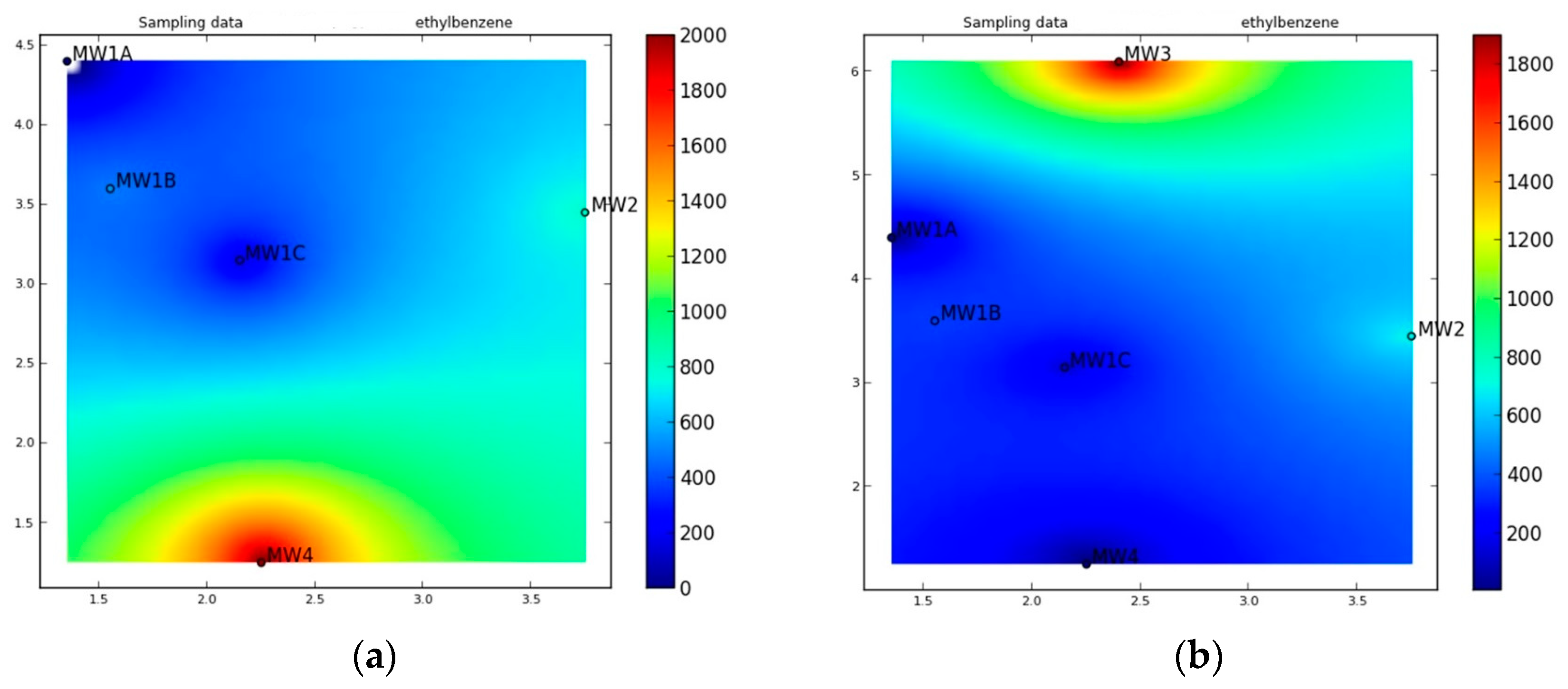
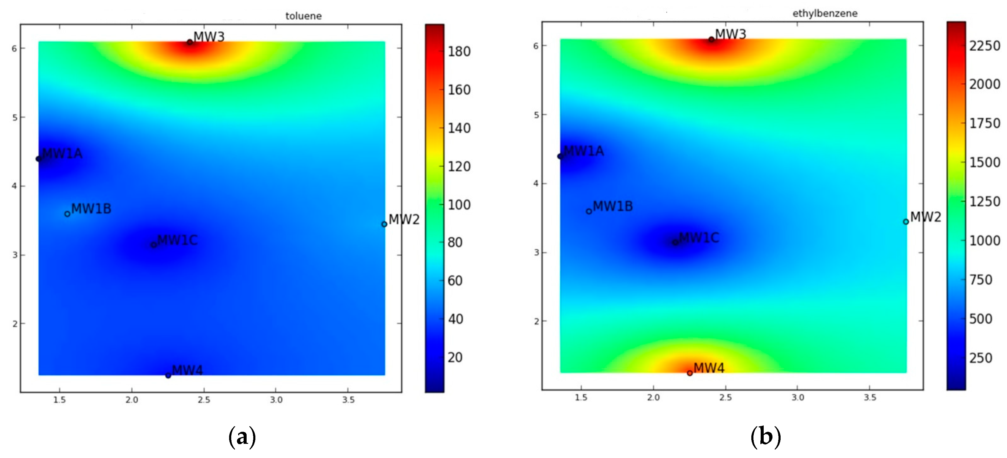
A monitoring of the baseline parameters showed a significant increase in the pH up to 11 in MW1A 5 days after injection. The front of the higher pH values (between 7 and 9) extended across the area from the borehole MW1 eastwards to MW2 approximately two weeks after injection (Figure 4), which could indicate the flow of the oxidising agent. The first sampling campaign after injection showed the highest temperature in MW1B with up to 16.2 °C. Two weeks after injection, the temperature remained high and fluctuated between 16 and over 18 °C, which could indicate the spread of the oxidising agent to the east (Figure 5). Measurements of toluene showed slightly elevated and dispersed concentrations of this pollutant immediately after injection and a decrease during the next sampling campaign over almost the entire area, which was direct evidence that the oxidiser was targeting this pollutant. High concentrations of this pollutant were only detected in the northern part of the area, which can be explained by a lateral flow of the pollutant from the source or by the effect of the rebound from the more impermeable soils (Figure 6).
Ethylbenzene was the most problematic COEC in the study area, with measurements a few days after the injection showing very high concentrations in the south and relatively low concentrations in the rest of the study area (Figure 7). Two weeks after the event, the trend reversed while ethylbenzene concentrations remained low in the centre, which can be explained by the spread of the oxidant. In the northern part, the concentrations were still very high, which was probably due to the rebound of the pollutants as, during the last sampling campaign (not shown), the amount of ethylbenzene increased both near the southern and the northern border.
Maps for the modelled values of the various parameters can also be displayed. In general, the geochemical model showed a quite good accuracy with respect to the spatial phenomena related to the injection of the oxidising agent. With regard to toluene, for example, the model showed both the consumption of the oxidising agent and the decreasing concentration of this pollutant in the central part of the study area and the rebound in the vicinity of well MW3 to the values observed during the sampling campaigns. The model also showed stable and low concentrations of ethylbenzene near the injection well and a recovery in the more distant wells, but the modelled recovery wave was delayed by about 10 days compared to the last sampling campaign (Figure 8). To summarise, the maps of the COECs and other parameters based on observed data can be very helpful for delineating zones where the oxidation is progressing from areas to where the process is not progressing satisfactorily due to unexpected circumstances such as rebound or strong heterogeneity. In addition, the spatial distribution of the predicted concentrations based on the model could prepare operators for such oxidation resistance before it is observed, thus allowing experts to plan further actions based on the model’s response before the problem is confirmed by measurements. In the case of the site in Flanders, the model showed that COEC concentrations in the northern and southern parts of the area were rising again due to desorption or ion exchange.
The user can view changes in the modelled parameters as XY graphs for the selected monitoring points or as a function of distance from the injection site. Below is an example graph showing the changes in pH versus the ROI distance and over multiple time intervals from 38 min to 89 days post-injection. According to the model, the pH increases from an initial value of about 8 to 9.2 at a reaction front immediately after injection (Figure 9). Within the radius of the influence, the pH is high until about one month after the start of treatment. The model predicted a drop in the pH at the edge of the ROI after 55 days, and the pH could drop to a value of 7 at a distance of 2.5 m from the injection after three months.
Similar to the pH plot, a very useful picture can be drawn from the model results, namely the consumption of permanganate within the ROI for different time periods after injection (Figure 10), from minutes to days, which takes into account the oxidation of both COECs and NOD, as well as the influx of background water and contaminants from the micropores’ water. As you can see, the model shows that, 3 months after the injection, the permanganate concentration near the injection site was almost a third of the original amount and close to 0 in the area more than 2 m away from this site.
3.2.4. Calibration of the Geochemical Model
The uncertainties of the model arise in the design phase, which is when the entire remediation plan must be encapsulated in a mathematical formulation and the response of the system to the input of the oxidising agent must be taken into account. In addition, there are two main sources of uncertainty in geochemical modelling: the choice of thermodynamic database or kinetic data and the choice of secondary minerals used in the model [87,88,89]. In the elaborated model, the definition of mineral composition was not the case as the dissolution and precipitation of minerals was not simulated. However, an initial uncertainty in the data was present because the oxidation reaction was kinetically controlled and the rates for each component subjected to oxidation must be specified. The uncertainties in the conceptual work phase were reduced by the knowledge of experts and practitioners, while the calibration of the model helped to reduce the uncertainties in the kinetic data.
The PHRREQC model could be calibrated/fitted to the following: (i) field data obtained during periodic monitoring, (ii) the laboratory test results and the literature data at, for example, the ISCO design stage, and (iii) real-time monitoring data. The model presented here combines all types of model validation. First, the model was developed using the available literature data, and the kinetic data controlling the dynamics of the oxidation process of both NOD and COECs were necessary and extremely important for building the reactive model. The model was then validated using real-time measurements and periodic chemical analyses at the ISCO injection site.
The real-time measurements included several parameters: pH, temperature, and the oxidation–reduction potential. As ISCO is very dynamic and, in some cases, unpredictable, the fitting of these parameters to the modelled values was based on a similar response to the arrival of the oxidant rather than on accuracy measures. Plots generated by the tool were used to visually check the observed and measured values.
For example, Figure 11 and Figure 12 show a comparison of the redox potential and pH measured by loggers in monitoring wells, and it was simulated by the hydrogeochemical model. The general patterns of chemical processes were reproduced with satisfactory accuracy. In some cases, due to soil heterogeneity, the propagation of oxidants in a real injection was delayed compared to the simulated one. However, on long time scales (i.e., weeks, months) such shifts were of minor importance. Of course, in some wells, due to very invasive conditions, the sensors showed abnormal values of some parameters, as described in Section 3.2.2. This was reported to the operators, and the equipment was subsequently checked.
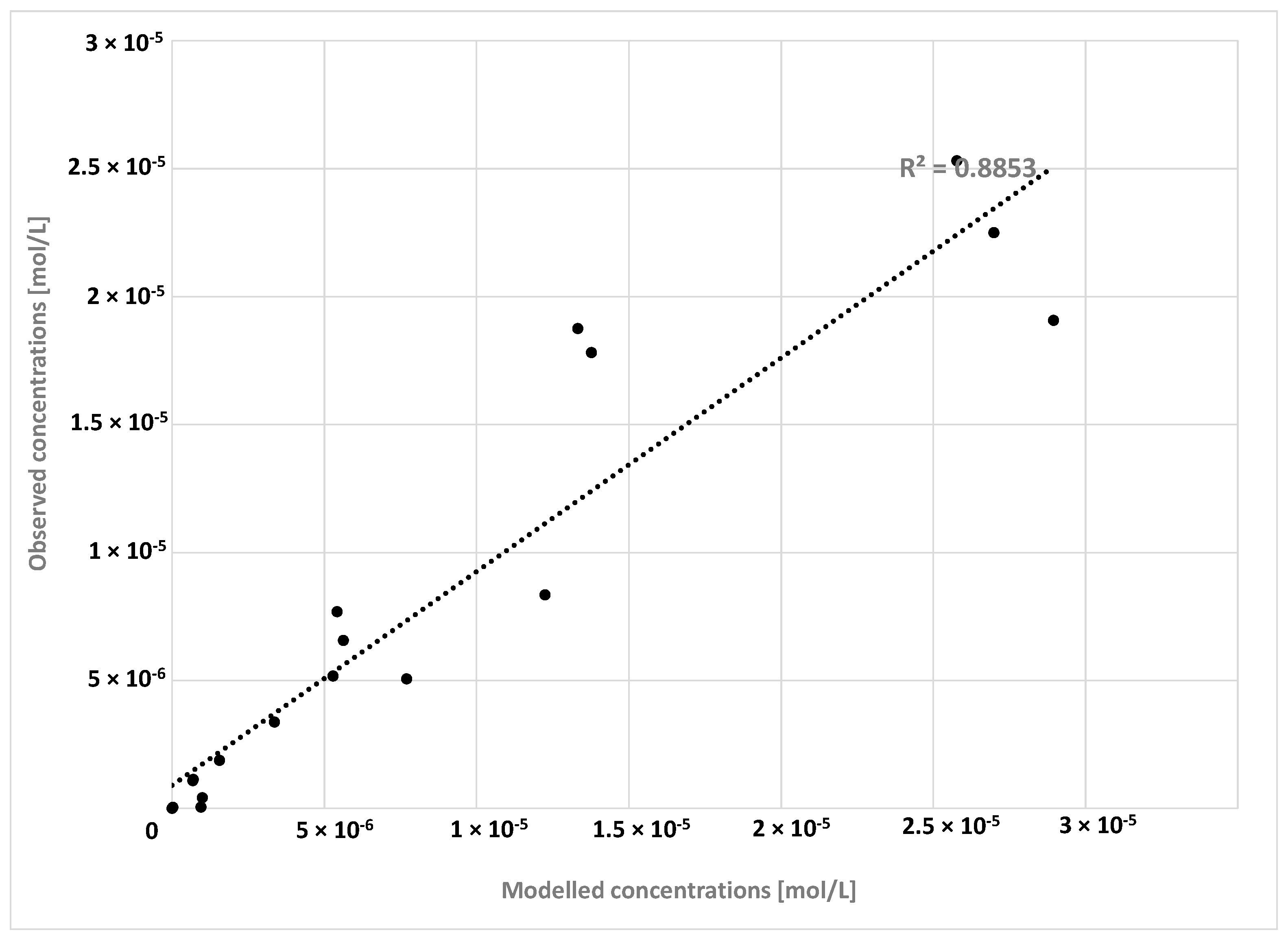
In addition, and more importantly, the model reflected with good accuracy the concentrations of the COECs immediately after injection and during the post-injection phase, when the rebound of contaminants can occur. The modelled values of the three BTEXs, toluene, benzene, and ethylbenzene, were compared with observations made over a few days, at one month, and at two months after injection. The measured values were successfully matched to the modelled values in a calibration that included changes in the contaminant concentrations in the micropores and the reaction rates of the BTEX oxidation. The latter was performed using the available literature sources. It should be noted that the injection conditions deviated from the ideal and controllable conditions of the laboratory experiment. During the recognition of the geological conditions, it turned out that, within the aquifer, there were layers of more impervious soils, which can be the secondary sources of contaminants when desorption occurs, and it was also noted that the heterogeneity of the matrix could affect the movement of the oxidant. However, the model consisting of two phases, injection and post-injection, gave good results over a two-month period and very variable concentrations of BTEX (Figure 13, Figure 14 and Figure 15). The Pearson correlation coefficients between the observed and modelled values were 0.81, 0.88, and 0.88 for benzene, toluene, and ethylbenzene, respectively. However, the lowest values reflected the fit of the pollutants occurring at very low concentrations (Figure 13).
Table 5 shows the comparison of the initial (theoretical) and calibrated (mean and median) values for the kinetic rates of the COEC oxidation by permanganate. The rates changed well during the calibration for each monitoring, but the changes between monitoring points were not large. It should be noted that the calibration gave much lower values for the oxidation rate of ethylbenzene than those adapted from the ISCOKIN database.
4. Discussion and Conclusions
The problem of soil and groundwater pollution from the extraction, transport, use, and processing of hydrocarbons is expected to increase as demand grows. Consumption of petroleum hydrocarbons is expected to rise to 106.6 million barrels by the end of 2030 [90]. Today, there are millions of contaminated sites in Europe alone, only a tiny fraction of which have been remediated. According to some reports, almost 9 million tonnes of oil are discharged into aquatic environments worldwide every year [91].
Many organic pollutants pose a major environmental threat to natural ecosystems and human health, and the long-term sources of residual contamination occur due to their persistence, solidification, and tendency in becoming trapped [92,93,94]. Therefore, the identification of contaminant sources and the selection of the best removal/treatment method and control of the entire process is a global issue [95,96]. The endeavour to remove contaminants and develop the most environmentally neutral methods of treating soil and groundwater is not only about current conditions and compliance with current standards, but also about long-term sustainability goals [97,98], which thus forces us to think about future needs and resource scarcity.
Natural attenuation processes are being considered as a method of remediating sites contaminated with hydrocarbons. They have the advantage of being inexpensive and having little impact on the environment, but they tend to be slow, so they often need to be improved and their efficiency studied in order to achieve satisfactory levels of removal in a reasonable time [99,100,101]. On the other hand, the pump-and-treat method is costly, long-term, and complicated [102]. Therefore, there is still room for cost-effective and smart in situ technologies that are faster and can be adapted to different sites and COECs [103,104]. In parallel with the development of treatment methods, increasingly sophisticated monitoring and risk assessment tools are being developed. The near real-time flow of information between devices, modelling tools, and operators could significantly improve the effectiveness of remediation. Key to this is not only communication between databases collecting information and modelling, but also trained experts and feedback from stakeholders [97].
The ISCO method is becoming increasingly popular, but this growing importance is not reflected in the modelling tools available to help experts in the field. To fill this gap, a tool based on the open-source software PHREEQC 2.18.0 and the Python language was developed. This article focuses on this user-friendly tool, which offers data storage and visualisation, simple remote control functions, and real-time and predictive responses to oxidant injection.
Firstly, all practitioners know that good planning and minimising the risk of failure is the key to a successful ISCO. Even a short plan that includes all site-specific information, targets, and the required oxidiser dose can be very helpful in achieving good reagent delivery. To fulfil the expectations of practitioners, the aforementioned tool includes a brief calculation of critical ISCO parameters such as the radius of influence, the actual velocity of groundwater mixed with the oxidant, and the volume of contaminated soil. Operators are also informed in real time about unexpected events and the arrival of the oxidising agent based on basic physical parameters. Since a picture is worth a thousand words, the advantage of this modelling tool is that the visualisation function, which also uses the Python language, facilitates the display of maps and XY plots of the observed and modelled data. This makes it possible to inform those responsible for remediation sites about what is really going on underground and to help them make further decisions.
The main feature of the described tool is the hydrogeochemical model PHREEQC, which could be used to predict oxidant consumption within the expected impact radius and to predict pollutant degradation. The reactive transport model could be run prior to the injection as part of the design plan and during ongoing treatment, which is supported by calibration. The hydrogeochemical model allows for the prediction of changes in groundwater chemical status in two phases: injection until ROI is reached and a user-defined post-injection period during which the rebound of COECs could be predicted if the ion exchange in microporous water is added to the simulations. The latter could be crucial for long-term land use planning and the application of other remediation methods.
It should be emphasised that the tool described is site-specific. It collects a variety of data specific to the area to be revitalised, such as background data on groundwater, contamination levels, and soil properties. In addition, soil structural heterogeneity is also taken into account by including hydraulic conductivity for each monitoring well, as well as by estimating groundwater velocity for each point where the oxidant release is observed and, more importantly, the actual velocity can be estimated based on the oxidant arrival for each observation point. COEC concentrations are also reported for each monitoring well.
The following conclusions can be made:
- The widely used PHREEQC code, Excel, and the Python programming language were combined to create a user-friendly and intuitive tool for researchers and practitioners in the field of in situ chemical oxidation;
- The concept of the tool is feedback-orientated, i.e., it is intended to provide the expert on site with direct feedback;
- The use of real-time and regular monitoring and modelling provides scientists, practitioners, and managers with a good knowledge base and helps to improve the effectiveness of remedial measures;
- The proposed tool was successfully tested at the contaminated site to check all functions. The tool informs about the unexpected conditions (alarm), the arrival of the oxidant (visualisation), and the time needed to reduce COEC and to consume the oxidant (geochemical model);
- The developed tool helps to address two phenomena that are crucial for the remediation and fate of solutes: heterogeneity and the rebound of contaminants;
- The geochemical model was successfully calibrated, and the kinetic data were slightly modified during the process. The adjusted values could also be valuable for researchers as they fit the field conditions better than the values determined under controllable laboratory conditions;
- The development of tools that are free, based on open-source software, and are open to change is crucial for reducing costs and sharing experiences.
The authors see opportunities for the presented tool to help ISCO practitioners improve the performance of this method. The presented tool can be further developed with regard to the use of other oxidising agents and tests at sites contaminated with other substances.
Supplementary Materials
The following supporting information can be downloaded at: https://www.mdpi.com/article/10.3390/app14093600/s1, Table S1: Simple outcomes from the tool, a set of equations and reactions.
Author Contributions
Conceptualisation, K.S.-G. and R.U.; methodology, K.S.-G. and R.U.; software PHREEQC 2.18.0, Python 3.7.0, K.S.-G. and R.U.; validation, K.S.-G.; formal analysis, K.S.-G.; investigation, K.S.-G. resources, K.S.-G. and R.U.; data curation, K.S.-G.; writing—original draft preparation, K.S.-G.; writing—review and editing, K.S.-G. and M.P.; visualisation, K.S.-G.; supervision, K.S.-G.; project administration, J.K.; funding acquisition, J.K. All authors have read and agreed to the published version of the manuscript.
Funding
The first version of the tool was developed with funding from the Seventh Framework Programme of the European Community (FP7/2007-2013) under grant agreement no. 226956. The Institute for Ecology of Industrial Areas also supported the development of the PHREEQC-based ISCO tool.
Institutional Review Board Statement
Not applicable.
Informed Consent Statement
Not applicable.
Data Availability Statement
The raw data supporting the conclusions of this article will be made available by the authors on request.
Acknowledgments
Special thanks are due to David Parkhurst for answering all the questions we had on geochemical modelling. The authors are grateful to Janek Greskowiak and Ondra Sracek for their constructive comments. The authors would like to thank Michał Szot for help with coding. Special thanks are given to the anonymous reviewers whose words of encouragement and comments helped to improve the manuscript and determine the future direction of the studies.
Conflicts of Interest
The authors declare no conflicts of interest.
References
- Environmental Protection Agency (EEA). Progress in Management of Contaminated Sites (csi 015) Assessment. 2007. Available online: https://www.eea.europa.eu/data-and-maps/indicators/progress-in-management-of-contaminated-sites-3/assessment (accessed on 16 February 2024).
- Van Liedekerke, M.; Prokop, G.; Rabl-Berger, S.; Kibblewhite, M.; Louwagie, G. Progress in the Management of Contaminated Sites in Europe; EUR 26376; Publications Office of the European Union: Luxembourg, 2014; 68p. [Google Scholar]
- Doust, H.G.; Huang, J.C. The fate and transport of hazardous chemicals in the subsurface environment. Water Sci. Technol. 1992, 25, 169–176. [Google Scholar] [CrossRef]
- US EPA. Engineered Approaches to In Situ Bioremediation of Chlorinated Solvents: Fundamentals and Field Applications; EPA-542-R-00-008; US EPA: Cincinnati, OH, USA, 2000.
- Siegrist, R.L.; Crimi, M.; Simpkin, T.J. (Eds.) In Situ Chemical Oxidation for Groundwater Remediation; Springer Science+Business Media, LLC: New York, NY, USA, 2011. [Google Scholar]
- Sharma, I. Bioremediation techniques for polluted environment: Concept, advantages, limitations, and prospects. In Trace Metals in the Environment-New Approaches and Recent Advances; IntechOpen: London, UK, 2020. [Google Scholar]
- Alori, E.T.; Gabasawa, A.I.; Elenwo, C.E.; Agbeyegbe, O.O. Bioremediation techniques as affected by limiting factors in soil environment. Front. Soil Sci. 2022, 2, 937186. [Google Scholar] [CrossRef]
- Ossai, I.C.; Ahmed, A.; Hassan, A.; Hamid, F.S. Remediation of soil and water contaminated with petroleum hydrocarbon: A review. Environ. Technol. Innov. 2020, 17, 100526. [Google Scholar] [CrossRef]
- Krembs, F.J. Critical Analysis of the Field Scale Application of In Situ Chemical Oxidation for the Remediation of Contaminated Groundwater. Master’s Thesis, Colorado School of Mines, Golden CO, USA, 2008; 223p. [Google Scholar]
- Ciampi, P.; Esposito, C.; Cassiani, G.; Deidda, G.P.; Rizzetto, P.; Papini, M.P. A field-scale remediation of residual light non-aqueous phase liquid (LNAPL): Chemical enhancers for pump and treat. Environ. Sci. Pollut. Res. 2021, 28, 35286–35296. [Google Scholar] [CrossRef]
- Trulli, E.; Morosini, C.; Rada, E.C.; Torretta, V. Remediation in situ of hydrocarbons by combined treatment in a contaminated alluvial soil due to an accidental spill of LNAPL. Sustainability 2016, 8, 1086. [Google Scholar] [CrossRef]
- Interstate Technology & Regulatory Council. Technical and Regulatory Guidance for In Situ Chemical Oxidation of Contaminated Soil and Groundwater, 2nd ed.; Interstate Technology & Regulatory Council: Washington, DC, USA, 2005. [Google Scholar]
- Liptak, L.; Nay, M.; Stewart, B. Peroxone Demonstration, Performance and Cost Evaluation; Aberdeen Proving Ground: Harford County, MD, USA, 1998. [Google Scholar]
- Huling, S.G.; Pivetz, B.E. Engineering Issue Paper: In-Situ Chemical Oxidation; EPA 600-R-06-072; U.S. EPA: Cincinnati, OH, USA, 2006.
- REGENESIS. Principles of Chemical Oxidation Technology for the Remediation of Groundwater and Soil, RegenOx™ Design and Application Manual—Version 2.0; REGENESIS: San Clemente, CA, USA, 2007. [Google Scholar]
- Tsitonaki, A.; Petri, B.; Crimi, M.; Mosbaek, H.A.N.S.; Siegrist, R.L.; Bjerg, P.L. In situ chemical oxidation of contaminated soil and groundwater using persulfate: A review. Crit. Rev. Environ. Sci. Technol. 2010, 40, 55–91. [Google Scholar] [CrossRef]
- Devi, P.; Das, U.; Dalai, A.K. In-situ chemical oxidation: Principle and applications of peroxide and persulfate treatments in wastewater systems. Sci. Total Environ. 2016, 571, 643–657. [Google Scholar] [CrossRef]
- Yang, Z.H.; Verpoort, F.; Dong, C.D.; Chen, C.W.; Chen, S.; Kao, C.M. Remediation of petroleum-hydrocarbon contaminated groundwater using optimized in situ chemical oxidation system: Batch and column studies. Process Saf. Environ. Prot. 2020, 138, 18–26. [Google Scholar] [CrossRef]
- Wei, K.H.; Ma, J.; Xi, B.D.; Yu, M.D.; Cui, J.; Chen, B.L.; Li, Y.; Gu, Q.-B.; He, X.S. Recent progress on in-situ chemical oxidation for the remediation of petroleum contaminated soil and groundwater. J. Hazard. Mater. 2022, 432, 128738. [Google Scholar] [CrossRef]
- Seol, Y.; Zhang, H.; Schwartz, F.W. A review of in situ chemical oxidation and heterogeneity. Environ. Eng. Geosci. 2003, 9, 37–49. [Google Scholar] [CrossRef]
- Pac, T.J.; Baldock, J.; Brodie, B.; Byrd, J.; Gil, B.; Morris, K.A.; Nelson, D.; Parikh, J.; Santos, P.; Singer, M.; et al. In situ chemical oxidation: Lessons learned at multiple sites. Remediat. J. 2019, 29, 75–91. [Google Scholar] [CrossRef]
- Baciocchi, R.; D’Aprile, L.; Innocenti, I.; Massetti, F.; Verginelli, I. Development of technical guidelines for the application of in-situ chemical oxidation to groundwater remediation. J. Clean. Prod. 2014, 77, 47–55. [Google Scholar] [CrossRef]
- Huling, S.G.; Ross, R.R.; Prestbo, K.M. In Situ Chemical Oxidation: Permanganate Oxidant Volume Design Considerations. Ground Water Monit Remediat. 2017, 37, 78–86. [Google Scholar] [CrossRef] [PubMed]
- Dangi, M.B.; Urynowicz, M.A.; Schultz, C.L.; Budhathoki, S. A comparison of the soil natural oxidant demand exerted by permanganate, hydrogen peroxide, sodium persulfate, and sodium percarbonate. Environ. Chall. 2022, 7, 100456. [Google Scholar] [CrossRef]
- McGachy, L.; Sedlak, D.L. From Theory to Practice: Leveraging Chemical Principles to Improve the Performance of Peroxydisulfate-Based In Situ Chemical Oxidation of Organic Contaminants. Environ. Sci. Technol. 2023, 58, 17–32. [Google Scholar] [CrossRef]
- Pac, T.; Cohen, E.; Crimi, M.; Dombrowski, P.; Duffy, B.; Lee, M.; Klemmer, M.; Pittenger, D.S.; Robinson, L. Remedial safety in in-situ chemical oxidation, crucial to success. Remediat. J. 2022, 32, 195–209. [Google Scholar] [CrossRef]
- Watts, R.J. Enhanced Reactant-Contaminant Contact through the Use of Persulfate In Situ Chemical Oxidation (ISCO); SERDP Project ER-1489; Washington State University: Pullman WA, USA, 2011. [Google Scholar]
- Bellamy, W.D.; Hickman, P.A.; Ziemba, N. Treatment of VOC-contaminated groundwater by hydrogen peroxide and ozone oxidation. J. Water Pollut. Control Federation 1991, 63, 120–128. [Google Scholar]
- Gates, D.D.; Siegrist, R.L. In situ chemical oxidation of trichloroethylene using hydrogen peroxide. J. Environ. Eng. 1995, 121, 639–644. [Google Scholar] [CrossRef]
- US EPA. Field Applications of In Situ Remediation Technologies: Chemical Oxidation; EPA 542-R-98-008; US EPA: Washington, DC, USA, 1998.
- US EPA. Ground Water Cleanup: Overview of Operating Experience at 28 Sites; EPA 542-R-99-006; US EPA: Washington, DC, USA, 1999.
- Yan, Y.E.; Schwartz, F.W. Oxidative degradation and kinetics of chlorinated ethylenes by potassium permanganate. J. Contam. Hydrol. 1999, 37, 343–365. [Google Scholar] [CrossRef]
- Gates-Anderson, D.D.; Siegrist, R.L.; Cline, S.R. Comparison of potassium permanganate and hydrogen peroxide as chemical oxidants for organically contaminated soils. J. Environ. Eng. 2001, 127, 337–347. [Google Scholar] [CrossRef]
- Interstate Technology & Regulatory Council. Technical and Regulatory Guidance for In Situ Chemical Oxidation of Contaminated Soil and Groundwater, 1st ed.; Interstate Technology & Regulatory Council: Washington, DC, USA, 2001. [Google Scholar]
- Siegrist, R.L. Principles and Practices of In Situ Chemical Oxidation Using Permanganate; Battelle Press: Columbus, OH, USA, 2001. [Google Scholar]
- Kim, J.; Choi, H. Modelling in situ ozonation for the remediation of nonvolatile PAH contaminated unsaturated soils. J. Contam. Hydrol. 2002, 55, 261–285. [Google Scholar] [CrossRef] [PubMed]
- NRC. Contaminants in the Subsurface: Source Zone Assessment and Remediation; National Academies Press: Washington, DC, USA, 2005. [Google Scholar]
- Bennedsen, L.R. In situ chemical oxidation: The mechanisms and applications of chemical oxidants for remediation purposes. In Chemistry of Advanced Environmental Purification Processes of Water; Elsevier: Amsterdam, The Netherlands, 2014; pp. 13–74. [Google Scholar]
- Clayton, W.S. Ozone and contaminant transport during in-situ ozonation. In Physical, Chemical, and Thermal Technologies: Remediation; Hinchee, G.B., Wickramanayake, R.E., Eds.; Battelle Press: Columbus, OH, USA, 1998; pp. 389–395. [Google Scholar]
- Hsu, I.-Y.; Masten, S.J. Modelling transport of gaseous ozone in unsaturated soils. J. Environ. Eng. 2001, 127, 546–554. [Google Scholar] [CrossRef]
- Sung, M.; Huang, C.P. In situ removal of 2-chlorophenol from unsaturated soils by ozonation. Environ. Sci. Technol. 2002, 36, 2911–2918. [Google Scholar] [CrossRef] [PubMed]
- Shin, W.-T.; Garanzuay, X.; Yiacoumi, S.; Tsouris, C.; Gu, B.; Mahinthakumar, G. Kinetics of soil ozonation: An experimental and numerical investigation. J. Contam. Hydrol. 2004, 72, 227–243. [Google Scholar] [CrossRef] [PubMed]
- Khan, N.A.; Carroll, K.C. Natural attenuation method for contaminant remediation reagent delivery assessment for in situ chemical oxidation using aqueous ozone. Chemosphere 2020, 247, 125848. [Google Scholar] [CrossRef] [PubMed]
- Hood, E.D. Permanganate Flushing of DNAPL Source Zones: Experimental and Numerical Investigation. Ph.D. Thesis, University of Waterloo, Waterloo, ON, USA, 2000. [Google Scholar]
- Zhang, H.; Schwartz, F.W. Simulating the in situ oxidative treatment of chlorinated ethylenes by potassium permanganate. Water Resour. Res. 2000, 36, 3031–3042. [Google Scholar] [CrossRef]
- Reitsma, S.; Dai, Q.L. Reaction-enhanced mass transfer and transport from non-aqueous phase liquid source zones. J. Contam. Hydrol. 2001, 49, 49–66. [Google Scholar] [CrossRef] [PubMed]
- Forsey, S.P. In Situ Chemical Oxidation of Creosote/Coal Tar Residuals: Experimental and Numerical Investigation. Ph.D. Thesis, University of Waterloo, Waterloo, ON, USA, 2004. [Google Scholar]
- Heiderscheidt, J.L. DNAPL Source Zone Depletion during In Situ Chemical Oxidation (ISCO): Experimental and Modelling Studies. Ph.D. Thesis, Colorado School of Mines, Golden, CO, USA, 2005. [Google Scholar]
- Mundle, K.; Reynolds, R.A.; West, M.R.; Kueper, B.H. Concentration rebound following in situ chemical oxidation in fractured clay. Groundwater 2007, 45, 692–702. [Google Scholar] [CrossRef] [PubMed]
- Henderson, T.H.; Ulrich, K.; Mayer, K.U.; Parker, B.L.; Al, T.A. Three-dimensional density dependent flow and multicomponent reactive transport modelling of chlorinated solvent oxidation by potassium permanganate. J. Contam. Hydrol. 2009, 106, 195–211. [Google Scholar] [CrossRef]
- Cha, K.Y.; Borden, R.C. Impact of injection system design on ISCO performance with permanganate—Mathematical modelling results. J. Contam. Hydrol. 2011, 128, 33–46. [Google Scholar] [CrossRef]
- Versteegen, F. Modelling Feedback Driven Remediation, a Modelling Study for the Monitoring of Efficiency, during KMnO4-Based In-Situ Chemical Oxidation of PCE Contamination; Deltares, Department Soil & Groundwater Systems: Utrecht, The Netherlands, 2011. [Google Scholar]
- Li, Y.; Yang, K.; Liao, X.; Cao, H.; Cassidy, D.P. Quantification of oxidant demand and consumption for in situ chemical oxidation design: In the case of potassium permanganate. Water Air Soil Pollut. 2018, 229, 355. [Google Scholar] [CrossRef]
- Evans, P.J.; Dugan, P.; Nguyen, D.; Lamar, M.; Crimi, M. Slow-release permanganate versus unactivated persulfate for long-term in situ chemical oxidation of 1, 4-dioxane and chlorinated solvents. Chemosphere 2019, 221, 802–811. [Google Scholar] [CrossRef] [PubMed]
- Chang, H.; Seaman, J.C.; Murphy, T.; Brown, S.; Mills, G. Laboratory and Modelling Efforts to Refine the use of In Situ Chemical Oxidation for Addressing Residual VOC Plumes on the Savannah River Site. In Proceedings of the 2011 Georgia Water Resources Conference, Athens, GA, USA, 11–13 April 2011. [Google Scholar]
- Peluffo, M.; Pardo, F.; Santos, A.; Romero, A. Use of different kinds of persulfate activation with iron for the remediation of a PAH-contaminated soil. Sci. Total Environ. 2016, 563–564, 649–656. [Google Scholar] [CrossRef] [PubMed]
- Chang, Y.-C.; Peng, Y.-P.; Chen, K.-F.; Chen, T.-Y.; Tang, C.-T. The effect of different in situ chemical oxidation (ISCO) technologies on the survival of indigenous microbes and the remediation of petroleum hydrocarbon-contaminated soil. Process Saf. Environ. Prot. 2022, 163, 105–115. [Google Scholar] [CrossRef]
- Han, M.; Wang, H.; Jin, W.; Chu, W.; Xu, Z. The performance and mechanism of iron-mediated chemical oxidation: Advances in hydrogen peroxide, persulfate and percarbonate oxidation. J. Environ. Sci. 2023, 128, 181–202. [Google Scholar] [CrossRef] [PubMed]
- Li, Y.; Chen, L.; Liu, Y.; Liu, F.; Fallgren, P.H.; Jin, S. Effects of bioaugmentation on sorption and desorption of benzene, 1, 3, 5-trimethylbenzene and naphthalene in freshly-spiked and historically-contaminated sediments. Chemosphere 2016, 162, 1–7. [Google Scholar] [CrossRef] [PubMed]
- Ranc, B.; Faure, P.; Croze, V.; Simonnot, M.O. Selection of oxidant doses for in situ chemical oxidation of soils contaminated by polycyclic aromatic hydrocarbons (PAHs): A review. J. Hazard. Mater. 2016, 312, 280–297. [Google Scholar] [CrossRef] [PubMed]
- Haselow, J.S.; Siegrist, R.L.; Crimi, M.; Jarosch, T. Estimating the total oxidant demand for in situ chemical oxidation design. Remediat. J. J. Environ. Cleanup Costs Technol. Tech. 2003, 13, 5–16. [Google Scholar] [CrossRef]
- Barcelona, M.J.; Holm, T.R. Oxidation-reduction capacities of soil. Environ. Sci. Technol. 1991, 25, 1565–1572. [Google Scholar] [CrossRef]
- Mumford, K.G.; Thomson, N.R.; Allen-King, R.M. Bench-scale investigation of permanganate natural oxidant demand kinetics. Environ. Sci. Technol. 2005, 39, 2835–2840. [Google Scholar] [CrossRef]
- Hønning, J. Use of In Situ Chemical Oxidation with Permanganate in PCE-Contaminated Clayey till with Sand Lenses; Institute of Environment & Resources, Technical University of Denmark: Lyngby, Denmark, 2007. [Google Scholar]
- Borden, R.C.; Simpkin, T.; Lieberman, M.T. User’s Guide, Design Tool for Planning Permanganate Injection Systems; ESTCP Project ER-0626; ESTCP: Alexandria, VA, USA, 2010. [Google Scholar]
- Illangasekare, T.H.; Marr, J.M.; Siegrist, R.L.; Glover, K.C.; Moreno-Barbero, E.; Heiderscheidt, J.L.; Saenton, S.; Matthew, M.; Kaplan, A.R.; Kim, Y.; et al. Mass Transfer from Entrapped DNAPL Sources Undergoing Remediation: Characterization Methods and Prediction Tools SERDP Project No. CU-1294; Colorado School of Mines: Golden, CO, USA, 2006. [Google Scholar]
- Parkhurst, D.L.; Appelo, C.A.J. User’s Guide to PHREEQC (Version 2); Inv. Rep. 99-4259; USGS. Water Resour: Reston, VA, USA, 1999.
- Prommer, H.; Post, V.E.A. A Reactive Multicomponent Model for Saturated Porous Media, Version 2.0, User’s Manual; National Ground Water Association: Westerville, OH, USA, 2010. [Google Scholar]
- Zhai, Y.; Cao, X.; Jiang, Y.; Sun, K.; Hu, L.; Teng, Y.; Wang, J.; Li, J. Further discussion on the influence radius of a pumping well: A parameter with little scientific and practical significance that can easily be misleading. Water 2021, 13, 2050. [Google Scholar] [CrossRef]
- ISCOKIN Database. Available online: https://zenodo.org/records/3596102 (accessed on 8 March 2024).
- Jones, L.J. The Impact of NOD Reaction Kinetic on Treatment Efficiency. Master’s Thesis, University of Waterloo, Waterloo, ON, Canada, 2007. [Google Scholar]
- Urynowicz, M.A.; Balu, B.; Udayasankar, U. Kinetics of Natural Oxidant Demand by Permanganate in Aquifer Solids. J. Contam. Hydrol. 2008, 96, 187–194. [Google Scholar] [CrossRef] [PubMed]
- Lemaire, J.; Buès, M.; Kabeche, T.; Hanna, K.; Simonnot, M.O. Oxidant selection to treat an aged PAH contaminated soil by in situ chemical oxidation. J. Environ. Chem. Eng. 2013, 1, 1261–1268. [Google Scholar] [CrossRef]
- Cronk, G. Optimization of a chemical oxidation tratment train process for groundwater remediation. In Proceedings of the Battelle 5th International Conference on Remediation of Chlorinated and Recalcitrant Compounds, Monterey, CA, USA, 25 May 2006. [Google Scholar]
- Bardos, R.P.; Bakker, L.M.; Slenders, H.L.; Nathanail, C.P. Sustainability and remediation. In Dealing with Contaminated Sites: From Theory towards Practical Application; Springer: Dordrecht, The Netherlands, 2010; pp. 889–948. [Google Scholar]
- Seyedpour, S.M.; Janmaleki, M.; Henning, C.; Sanati-Nezhad, A.; Ricken, T. Contaminant transport in soil: A comparison of the Theory of Porous Media approach with the microfluidic visualisation. Sci. Total Environ. 2019, 686, 1272–1281. [Google Scholar] [CrossRef]
- Khan, S.; Naushad, M.; Lima, E.C.; Zhang, S.; Shaheen, S.M.; Rinklebe, J. Global soil pollution by toxic elements: Current status and future perspectives on the risk assessment and remediation strategies—A review. J. Hazard. Mater. 2021, 417, 126039. [Google Scholar] [CrossRef]
- McInerny, G.J.; Chen, M.; Freeman, R.; Gavaghan, D.; Meyer, M.; Rowland, F.; Spiegelhalter, D.J.; Stefaner, M.; Tessarolo, G.; Hortal, J. Information visualisation for science and policy: Engaging users and avoiding bias. Trends Ecol. Evol. 2014, 29, 148–157. [Google Scholar] [CrossRef] [PubMed]
- Azpurua, M.; Dos Ramos, K. A comparison of spatial interpolation methods for estimation of average electromagentic field magnitude. Prog. Electromagn. Res. 2010, 14, 135–145. [Google Scholar] [CrossRef]
- Yu, A.; Chung, C.; Yim, A. Matplotlib 2. x By Example; Packt Publishing Ltd.: Birmingham, UK, 2017. [Google Scholar]
- Van Rossum, G.; Drake, F.L. Python Tutorial, Release 2.7.3; Python Software Foundation: Wilmington, DE, USA, 2012. [Google Scholar]
- Lu, G.Y.; Wong, D.W. An adaptive inverse-distance weighting spatial interpolation technique. Comput. Geosci. 2008, 34, 1044–1055. [Google Scholar] [CrossRef]
- Chen, F.W.; Liu, C.W. Estimation of the spatial rainfall distribution using inverse distance weighting (IDW) in the middle of Taiwan. Paddy Water Environ. 2012, 10, 209–222. [Google Scholar] [CrossRef]
- Masroor, K.; Fanaei, F.; Yousefi, S.; Raeesi, M.; Abbaslou, H.; Shahsavani, A.; Hadei, M. Spatial modelling of PM2. 5 concentrations in Tehran using Kriging and inverse distance weighting (IDW) methods. J. Air Pollut. Health 2020, 5, 89–96. [Google Scholar]
- Shukla, K.; Kumar, P.; Mann, G.S.; Khare, M. Mapping spatial distribution of particulate matter using Kriging and Inverse Distance Weighting at supersites of megacity Delhi. Sustain. Cities Soc. 2020, 54, 101997. [Google Scholar] [CrossRef]
- Dethlefsen, F.; Haase, C.; Ebert, M.; Dahmke, A. Uncertainties of geochemical modeling during CO2 sequestration applying batch equilibrium calculations. Environ. Earth Sci. 2012, 65, 1105–1117. [Google Scholar] [CrossRef]
- Mosai, A.K.; Tokwana, B.C.; Tutu, H. Computer simulation modelling of the simultaneous adsorption of Cd, Cu and Cr from aqueous solutions by agricultural clay soil: A PHREEQC geochemical modelling code coupled to parameter estimation (PEST) study. Ecol. Model. 2022, 465, 109872. [Google Scholar] [CrossRef]
- Poort, J.; De Zwart, H.; Wasch, L.; Shoeibi Omrani, P. The H2020 REFLECT Project: D4. 3 Impact of Geochemical Uncertainties on Fluid Production and Scaling Prediction; GFZ German Research Centre for Geosciences: Potsdam, Germany, 2022. [Google Scholar]
- Igunnu, E.T.; Chen, G.Z. Produced water treatment technologies. Int. J. Low-Carbon Technol. 2014, 9, 157–177. [Google Scholar] [CrossRef]
- Dadrasnia, A.; Agamuthu, P. Diesel fuel degradation from contaminated soil by Dracaena reflexa using organic waste supplementation. J. Jpn. Pet. Inst. 2013, 56, 236–243. [Google Scholar] [CrossRef]
- Uddin, S.; Fowler, S.W.; Saeed, T.; Jupp, B.; Faizuddin, M. Petroleum hydrocarbon pollution in sediments from the Gulf and Omani waters: Status and review. Mar. Pollut. Bull. 2021, 173, 112913. [Google Scholar] [CrossRef] [PubMed]
- Haider, F.U.; Ejaz, M.; Cheema, S.A.; Khan, M.I.; Zhao, B.; Liqun, C.; Salim, M.A.; Naveed, M.; Khan, N.; Nunez-Delgado, A.; et al. Phytotoxicity of petroleum hydrocarbons: Sources, impacts and remediation strategies. Environ. Res. 2021, 197, 111031. [Google Scholar] [CrossRef]
- Gatsios, E.; García-Rincón, J.; Rayner, J.L.; McLaughlan, R.G.; Davis, G.B. LNAPL transmissivity as a remediation metric in complex sites under water table fluctuations. J. Environ. Manag. 2018, 215, 40–48. [Google Scholar] [CrossRef] [PubMed]
- Kuppusamy, S.; Maddela, N.R.; Megharaj, M.; Venkateswarlu, K. Case studies on remediation of sites contaminated with total petroleum hydrocarbons. In Total Petroleum Hydrocarbons: Environmental Fate, Toxicity, and Remediation; Springer: Berlin/Heidelberg, Germany, 2020; pp. 225–256. [Google Scholar]
- Verardo, E.; Atteia, O.; Rouvreau, L.; Siade, A.; Prommer, H. Identifying remedial solutions through optimal bioremediation design under real-world field conditions. J. Contam. Hydrol. 2021, 237, 103751. [Google Scholar] [CrossRef]
- Syafiuddin, A.; Boopathy, R.; Hadibarata, T. Challenges and solutions for sustainable groundwater usage: Pollution control and integrated management. Curr. Pollut. Rep. 2020, 6, 310–327. [Google Scholar] [CrossRef]
- Ambaye, T.G.; Chebbi, A.; Formicola, F.; Prasad, S.; Gomez, F.H.; Franzetti, A.; Vaccari, M. Remediation of soil polluted with petroleum hydrocarbons and its reuse for agriculture: Recent progress, challenges, and perspectives. Chemosphere 2022, 293, 133572. [Google Scholar] [CrossRef] [PubMed]
- Da Silva, M.L.B.; Corseuil, H.X. Groundwater microbial analysis to assess enhanced BTEX biodegradation by nitrate injection at a gasohol-contaminated site. Int. Biodeterior. Biodegrad. 2012, 67, 21–27. [Google Scholar] [CrossRef]
- Balland-Bolou-Bi, C.; Brondeau, F.; Jusselme, M. Can Natural Attenuation be Considered as an Effective Solution for Soil Remediation? IntechOpen: Soil Contamination—Recent Advances and Future Perspectives. 2022. Available online: https://www.intechopen.com/online-first/84766 (accessed on 13 March 2024).
- Lv, H.; Su, X.; Wang, Y.; Dai, Z.; Liu, M. Effectiveness and mechanism of natural attenuation at a petroleum-hydrocarbon contaminated site. Chemosphere 2018, 206, 293–301. [Google Scholar] [CrossRef] [PubMed]
- Keely, J.F. Performance Evaluations of Pump-and-Treat Remediations 1. In EPA Environmental Engineering Sourcebook; CRC Press: Boca Raton, FL, USA, 2019; pp. 31–57. [Google Scholar]
- Cleland, J.; Leggett, H.; Sandars, J.; Costa, M.J.; Patel, R.; Moffat, M. The remediation challenge: Theoretical and methodological insights from a systematic review. Med. Educ. 2013, 47, 242–251. [Google Scholar] [CrossRef] [PubMed]
- Zhang, T.; Lowry, G.V.; Capiro, N.L.; Chen, J.; Chen, W.; Chen, Y.; Dionysiou, D.; Elliot, D.W.; Ghosal, S.; Hofmann, T.; et al. In situ remediation of subsurface contamination: Opportunities and challenges for nanotechnology and advanced materials. Environ. Sci. Nano 2019, 6, 1283–1302. [Google Scholar] [CrossRef]
- Grifoni, M.; Franchi, E.; Fusini, D.; Vocciante, M.; Barbafieri, M.; Pedron, F.; Rosellini, I.; Petruzzelli, G. Soil remediation: Towards a resilient and adaptive approach to deal with the ever-changing environmental challenges. Environments 2022, 9, 18. [Google Scholar] [CrossRef]
Figure 2.
Visualisation of the ICSO site. Location of the injection point (red dot) and monitoring wells (green dots). The labels show the monitoring well names and screen depths. The size of the monitoring wells was proportional to the depth of their screens.
Figure 2.
Visualisation of the ICSO site. Location of the injection point (red dot) and monitoring wells (green dots). The labels show the monitoring well names and screen depths. The size of the monitoring wells was proportional to the depth of their screens.

Figure 3.
Example of an alarm plot for monitoring well MW1A where the pH had exceeded the acceptable level at the start of injection (17 March) and then stabilised within the expected range.
Figure 3.
Example of an alarm plot for monitoring well MW1A where the pH had exceeded the acceptable level at the start of injection (17 March) and then stabilised within the expected range.

Figure 4.
Map showing the pH for (a) 5 days after the injection and (b) 20 days after the injection.
Figure 4.
Map showing the pH for (a) 5 days after the injection and (b) 20 days after the injection.

Figure 5.
Map showing the temperature (°C) for (a) 5 days after the injection and (b) 20 days after the injection.
Figure 5.
Map showing the temperature (°C) for (a) 5 days after the injection and (b) 20 days after the injection.

Figure 6.
Map showing toluene concentrations (μg/L) for (a) 5 days after the injection and (b) 20 days after the injection.
Figure 6.
Map showing toluene concentrations (μg/L) for (a) 5 days after the injection and (b) 20 days after the injection.

Figure 7.
Map showing the ethylbenzene concentrations (μg/L) for (a) 5 days after the injection and (b) 20 days after the injection.
Figure 7.
Map showing the ethylbenzene concentrations (μg/L) for (a) 5 days after the injection and (b) 20 days after the injection.

Figure 8.
Map showing the modelled concentrations (μg/L) for (a) toluene and (b) ethylbenzene almost two months after the injection.
Figure 8.
Map showing the modelled concentrations (μg/L) for (a) toluene and (b) ethylbenzene almost two months after the injection.

Figure 9.
Example of an XY plot as a result of the geochemical model showing modelled pH values as a function of the distance from the injection point for selected time stamps.
Figure 9.
Example of an XY plot as a result of the geochemical model showing modelled pH values as a function of the distance from the injection point for selected time stamps.

Figure 10.
Example of an XY plot as a result of the geochemical model showing modelled permanganate concentrations as a function of the distance from the injection point for selected time stamps.
Figure 10.
Example of an XY plot as a result of the geochemical model showing modelled permanganate concentrations as a function of the distance from the injection point for selected time stamps.

Figure 11.
Comparison of the redox potential measured in real time (with the TempHion sensor) and simulated by PHREEQC in the MW4 borehole.
Figure 11.
Comparison of the redox potential measured in real time (with the TempHion sensor) and simulated by PHREEQC in the MW4 borehole.

Figure 12.
Comparison of the pH measured in real time (TempHion) and simulated by PHREEQC in the MW2 borehole.
Figure 12.
Comparison of the pH measured in real time (TempHion) and simulated by PHREEQC in the MW2 borehole.

Figure 13.
Relationship between the observed benzene concentrations and PHREEQC model predictions.

Figure 14.
Relationship between the observed toluene concentrations and PHREEQC model predictions.

Figure 15.
Relationship between the observed ethylbenzene concentrations and PHREEQC model predictions.
Figure 15.
Relationship between the observed ethylbenzene concentrations and PHREEQC model predictions.

Table 1.
List of the processes and parameters used in kinetic calculations.
| Process | Second-Order Rate Constant [M−1s−1] | |
|---|---|---|
| PCE oxidation 1 | 0.038 | |
| TCE oxidation 1 | 0.67 | |
| DCE oxidation 1 | 2.32 | |
| VC oxidation 1 | 0.014–0.029 | |
| Benzene oxidation 1 | 7 × 10⁻⁶ | |
| Toluene oxidation 1 | 5.7 × 10⁻⁴ | |
| Ethylbenzene oxidation 1 | 0.007 | |
| NOD (organic matter) Oxidation 1 | Fast fraction | 2.54 × 10⁻¹⁰ |
| Slow fraction | 1.15 × 10⁻¹⁴ | |
1 Oxidation by permanganate.
Table 3.
Ranges of the basic parameters expected during the ISCO process.
| Parameters | Range [Source] |
|---|---|
| Temperature | Above 15 °C (10–15 °C is a typical for ambient water [5]) |
| pH | 2.5–12.5 [5] |
| Eh | +200 to +600 mV [75] |
Table 4.
Description of the test site parameters and ISCO procedure.
| Contaminated Area | ||
|---|---|---|
| Parameter | Values * | |
| Groundwater level | 1.33 ÷ 1.53 (avg. 1.45) m bgl. | |
| pH | 6.4 ÷ 8.2 (avg. 7.41) | |
| ORP | −286 ÷ 98 (avg. 35) mV | |
| Dissolved oxygen | 1.3 ÷ 2.9 (avg. 2.16) mg/L | |
| DOC | 75 ÷ 3710 (avg. 548) mg/L | |
| Eh | −0.286 ÷ 0.098 (avg. −0.035) V | |
| EC | 756 ÷ 5070 (avg. 1883) μS/cm | |
| Groundwater temperature | 9.8 ÷ 13.5 (avg. 11.8) °C | |
| Thickness of the contaminated layer | 1.5 m | |
| Depth to the impervious layer | 25 m | |
| Hydraulic conductivity | 7.25 × 10⁻⁸ ÷ 3.27 × 10⁻⁶ (avg. 9.4 × 10⁻⁷) m/s | |
| Porosity | 0.35 | |
| Dry bulk density | 1700 kg/m3 | |
| Toluene | 0.014 ÷ 0.17 (avg. 0.037) mg/L | |
| Ethylobenzene | 0.21 ÷ 6.8 (avg. 1.81) mg/L | |
| Benzene | 0.02 ÷ 0.002 (avg. 0.013) mg/L | |
| PCE | 0.05 mg/L | |
| TCE | 0.05 mg/L | |
| DCE | 0.05 ÷ 7.3 (avg. 1.26) mg/L | |
| VC | 0.05 ÷ 0.32 (avg. 0.12) mg/L | |
| NOD | 3792 mg/L | |
| C-chlorides | 220 ÷ 1080 (avg. 391) mg/L | |
| Parameter | Water in micropores | Clean Groundwater |
| Temperature | 14.7 °C | 12.7 °C |
| pH | 6.24 | 6.55 |
| Eh | 0.084 V | −0.061 V |
| Toluene | 0.8 mg/L | - |
| Ethylobenzene | 3.3 mg/L | - |
| Benzene | 0.05 mg/L | - |
| PCE | 1.7 mg/L | - |
| TCE | 0.4 mg/L | - |
| DCE | 10 mg/L | - |
| VC | 0.05 mg/L | 12.7 °C |
| Injection Parameter | Values | |
| Volume of the injected fluid | 1.2 m3 | |
| Concentration of the oxidant | 83 kg/m3 | |
| pH of the injected fluid | 7 | |
| Pe of the injected fluid | 15 | |
| Velocity of the natural lateral flow | 20 m/year | |
* One value if based on one sampling or min ÷ max (and the distance averaged for the centre of the injection area) or if based on multiple monitoring wells.
Table 5.
The initial and final values of the oxidation rates for the site in Flanders.
| COEC | Initial Second-Order Rate Constant [M−1s−1] | Second-Order Rate Constant after Calibration [M−1s−1] |
|---|---|---|
| Benzene | 7 × 10⁻⁶ | Mean 8.25 × 10⁻⁶ Median 7.25 × 10⁻⁶ |
| Toluene | 5.7 × 10⁻⁴ | Mean 1.4−4 Median 1 × 10⁻⁴ |
| Ethylbenzene | 0.007 | Mean 1.2−4 Median 7 × 10⁻⁵ |
Disclaimer/Publisher’s Note: The statements, opinions and data contained in all publications are solely those of the individual author(s) and contributor(s) and not of MDPI and/or the editor(s). MDPI and/or the editor(s) disclaim responsibility for any injury to people or property resulting from any ideas, methods, instructions or products referred to in the content. |
© 2024 by the authors. Licensee MDPI, Basel, Switzerland. This article is an open access article distributed under the terms and conditions of the Creative Commons Attribution (CC BY) license (https://creativecommons.org/licenses/by/4.0/).
Share and Cite
MDPI and ACS Style
Samborska-Goik, K.; Ulańczyk, R.; Krupanek, J.; Pogrzeba, M. A PHREEQC-Based Tool for Planning and Control of In Situ Chemical Oxidation Treatment. Appl. Sci. 2024, 14, 3600. https://doi.org/10.3390/app14093600
AMA Style
Samborska-Goik K, Ulańczyk R, Krupanek J, Pogrzeba M. A PHREEQC-Based Tool for Planning and Control of In Situ Chemical Oxidation Treatment. Applied Sciences. 2024; 14(9):3600. https://doi.org/10.3390/app14093600
Chicago/Turabian StyleSamborska-Goik, Katarzyna, Rafał Ulańczyk, Janusz Krupanek, and Marta Pogrzeba. 2024. "A PHREEQC-Based Tool for Planning and Control of In Situ Chemical Oxidation Treatment" Applied Sciences 14, no. 9: 3600. https://doi.org/10.3390/app14093600
Note that from the first issue of 2016, this journal uses article numbers instead of page numbers. See further details here.